The Use of Remotely Sensed Rainfall for Managing Drought Risk: A Case Study of Weather Index Insurance in Zambia

Abstract

Remotely sensed rainfall is increasingly being used to manage climate-related risk in gauge sparse regions. Applications based on such data must make maximal use of the skill of the methodology in order to avoid doing harm by providing misleading information. This is especially challenging in regions, such as Africa, which lack gauge data for validation. In this study, we show how calibrated ensembles of equally likely rainfall can be used to infer uncertainty in remotely sensed rainfall estimates, and subsequently in assessment of drought. We illustrate the methodology through a case study of weather index insurance (WII) in Zambia. Unlike traditional insurance, which compensates proven agricultural losses, WII pays out in the event that a weather index is breached. As remotely sensed rainfall is used to extend WII schemes to large numbers of farmers, it is crucial to ensure that the indices being insured are skillful representations of local environmental conditions. In our study we drive a land surface model with rainfall ensembles, in order to demonstrate how aggregation of rainfall estimates in space and time results in a clearer link with soil moisture, and hence a truer representation of agricultural drought. Although our study focuses on agricultural insurance, the methodological principles for application design are widely applicable in Africa and elsewhere.

1. Introduction

Monitoring of rainfall is essential for famine early warning and for the management of agricultural risk [1,2]. In many parts of the world the gauge station network is sparse, and hence monitoring cannot rely on ground-based measurements. An alternative is to use remotely sensed data, such as satellite-based rainfall estimates (i.e., rainfall that is estimated based on calibrated satellite imagery—for example, [3,4,5]). Although they both provide estimates of rainfall, satellite and ground-based methods are fundamentally different. Their agreement varies spatially and temporally, depending on the meteorological regime, satellite rainfall estimation methodology, and density of the gauge network [6,7,8,9].

The skill of remotely sensed rainfall estimates is generally improved by aggregating in time and space [10,11,12]. The more rainfall is aggregated, however, the less representative it becomes of local meteorological conditions. When deciding on a scale for aggregation, improvement in skill must be balanced against loss of “representativity” [13]. It is important to note, however, that not all applications that use rainfall data depend on instantaneous knowledge of local conditions. Indeed, applications based on temporally and spatially aggregated rainfall may be naturally suited to satellite-based rainfall monitoring. Agricultural losses, for example, are linked more closely to cumulative rainfall than to instantaneous rainfall at a point.

Assessments of the usefulness of remotely sensed rainfall thus need to account for the context in which the data are being used. Climate-related risk to agriculture is related both to variability in the weather and to the interaction between meteorological and land-surface conditions. The suitability of proxies, such as remotely sensed rainfall, depends, moreover, not only on skill in representing spatial and temporal variability, but also on the relative importance of this variability for the application in question.

In this paper, we illustrate these issues through a case study of the use of remotely sensed rainfall for weather index insurance (WII)—a form of drought insurance increasingly used in regions such as Africa and India. Unlike traditional insurance, which compensates proven loss, WII pays out in the event that a weather index is breached [14,15]. Lack of agricultural insurance in Africa increases the vulnerability of farmers to climate-related risk. WII has the potential to be cheap to administer and transparent to operate. In principle, WII provides a means of insuring smallholder farmers throughout Africa against drought. In a data-sparse region, such as Africa, expanding WII schemes requires the use of remotely sensed environmental data, including rainfall. Design of indices that maximise the skill of satellite-based rainfall estimates for the monitoring of agricultural drought is thus a pressing concern [16]. However, assessment of skill is challenging in regions, such as Africa, where the ground station network is sparse. And yet, these are the regions most dependent on remotely sensed rainfall [9]. Our case study presents a novel application of a well-established method for inferring uncertainties inherent in spatially and temporally aggregated remotely sensed rainfall [17,18,19].

A key issue for WII is the mismatch between insured weather based indices and agricultural losses. This can lead either to unfair payouts, or to uncompensated losses. Such mismatches are termed basis risk. Basis risk can result from losses that are not connected with variability in the weather. Cotton yield may, for example, be reduced by pests and diseases [20]. Another aspect of basis risk stems from complexities in the progression from below expected rainfall (meteorological drought), to deficit in root zone soil moisture (agricultural drought). Complexities arise because below expected rainfall is not necessarily a precursor to soil moisture deficit, and conversely, soil moisture deficits occur, even when rainfall is near normal [21,22]. Furthermore, if remotely sensed data are used, lack of skill in the estimation methodology can lead to errors in the indices themselves, and hence to increased basis risk. When designing indices based on remotely sensed rainfall, it is thus necessary to consider the propagation of uncertainty from errors in rainfall estimation to complexities in the link between rainfall and drought.

In this paper, we focus on cotton in Zambia–an economically important cash crop with highly variable yield (Figure 1), which is already insured using remotely sensed rainfall. It should be noted that cotton is sensitive not only to rainfall, and indeed that sensitivity to other meteorological parameters may increase basis risk for WII schemes that are based only on rainfall. For example, laboratory-based studies have demonstrated that cotton yield is adversely affected by heat stress, with optimal temperatures being about 28 °C and severe damage ensuing when temperatures exceed ~35 °C [23,24]. Nevertheless, field studies carried out in Africa, suggest that, while variability in temperature has a significant impact, rainfall variability is the dominant environmental driver of variation in yield [25].

In this study, we first use a land-surface model to describe the progression from meteorological to agricultural drought in the region. We then consider how aggregation in space and time affects the capacity of satellite-based rainfall estimates to represent local rainfall. The final part of the analysis draws these threads of analysis into a discussion of how the aggregation of rainfall relates to basis risk. The paper closes with a brief account of the bearing that the methodologies presented have on weather index design.

2. Data and Methods

This study combines land-surface model integrations with analyses of satellite imagery and survey of agricultural loss data. The land surface model chosen was the Joint UK Land Environment Simulator (JULES), the land surface model of the UK Met Office. JULES, driven with remotely sensed rainfall and reanalysis data, is used to investigate the development of drought and the scales of land-atmosphere interactions. Analysis of ensembles of equally likely rainfall is used to quantify algorithmic uncertainty in the rainfall estimates, and thus to quantify the effect of aggregation in space and time on skill. The following sections describe JULES, the satellite-based rainfall estimation methodology (Tropical Applications of Meteorology using SATellite and ground based data (TAMSAT)), and the agricultural loss data.

2.1. Representation of Agricultural Drought Using the Joint UK Land Environment Simulator (JULES)

JULES is a process-based land-surface model [26,27]. When coupled to one of the Hadley Centre atmosphere models, it comprises the land-surface scheme of the Hadley Centre climate models. Being a process-based model, JULES can be used to investigate the links between climatic and other environmental factors and the condition of the land surface [28,29]. In Zambia, where there are no long-term observations of root zone soil moisture, output from models such as from JULES can provide an indication of the nature of the links between the climate and the water available to plants. In this study, JULES is being used to infer the expected strength of the link between rainfall and agricultural drought in Zambia. The following summarizes the features of JULES that are of greatest relevance to this study.

JULES divides the land-surface into nine surface types: broadleaf trees, needle leaf trees, C3 grass, C4 grass, shrubs, urban, inland water, bare soil, and ice. The land-surface types are tiled to represent sub-grid heterogeneity [30]. Surface fluxes of moisture and heat are calculated for each tile, and the state of the grid box is then represented by the aggregation of the tile fluxes. JULES can be run either at a point or over a grid (distributed JULES). It is important to note that the formulation of distributed JULES used for this study does not include lateral transfer of heat or moisture.

JULES includes a multi-layer representation of soil. Each soil layer is described by a set of hydraulic and thermal properties (Table 3 in [26]). In practice, these quantities are derived by applying pedotransfer functions to maps of soil texture [31]. In distributed JULES, the soil hydraulic and thermal properties are allowed to vary from one grid point to another. Although it is possible to vary the soil properties with depth, for this study, they were assumed to be constant. The calculation of soil moisture is described in detail in the published descriptions of JULES [26,27]. The following summarizes the key processes. The soil moisture in the top layer of soil is related to the amount of water that reaches the soil, the maximum rate of infiltration and the rate of evaporation. For non-vegetated surfaces, the amount of water reaching the soil is equivalent to the precipitation. For vegetated surfaces, the amount of water reaching the soil is the canopy throughfall. The calculation of canopy throughfall in JULES accounts for precipitation, the water held in the canopy, and the rate of evaporation from the canopy water store (Equations (46) and (47) in [26]). Once water reaches the surface, it either infiltrates, or runs off. The gridbox runoff rate is given by Equation (48) in [26] and derived in [32]. The infiltration is then calculated from the water balance.

In JULES, water can move vertically through the soil layers, and can drain from the lowest layer. The fluxes of water between layers are calculated using the finite difference formulation of the Richards equation:

$$\frac{d\theta }{dt}=w_{k-1}-w_k-E_K-R_K$$

(1)

where W_k-1 and W_k are the diffusive fluxes of water flowing into and out of soil layer k, E_k is the moisture extracted by plant roots from the lower layers, or evaporated from the top layer. In this study, the soil column is split into four layers (depths 0.1, 0.25, 0.65, and 2 metres). Note that the lateral runoff (R_k) is set to zero.

The water availability to plants (beta) is a function of the soil moisture concentration (see above), the soil moisture concentration at the critical point and the soil moisture concentration at the wilting point. The critical point is the soil moisture concentration below which plants start to be affected by water stress. When soil moisture is lower than the wilting point, plants do not grow or transpire. The critical and wilting points depend on soil texture [26].

The formulation of beta is given in Equation (2), where θ is the soil moisture concentration, θ_w is the soil moisture concentration at the wilting point and θ_c is the soil moisture at the critical point. Beta ranges from 0 to 1. When beta is 1, modelled plant growth is not affected by water stress.

$$\beta =\{\begin{array}{ll}1\hfill & \theta \ge {\theta }_c\hfill \\ \frac{\theta -{\theta }_w}{{\theta }_c-{\theta }_w}\hfill & {\theta }_w<\theta <{\theta }_c\hfill \\ 0\hfill & \theta \le {\theta }_w\hfill \end{array}$$

(2)

Beta is directly related to the water stress on plants, and can thus be used to infer the degree of agricultural drought as the season progresses. The link between beta and rainfall, moreover, reflects the link between agricultural and meteorological drought.

The results shown in Section 3 derive from integrations of JULES carried out for 1983–2012 at 0.5° horizontal resolution over the illustrated horizontal domain shown. JULES was forced with three-hourly gridded time series of radiation, precipitation, temperature, humidity, wind speed, and surface pressure, extracted from the WFDEI (WATCH Forcing Data based on ERA-Interim) forcing dataset [33]. In this dataset, all variables apart from precipitation are extracted from the WFDEI dataset; the precipitation data are TAMSAT rainfall ensembles (see Section 2.2). The land cover surface type percentages and the soil properties at each grid point were provided as part of the WFDEI dataset [33].

2.2. TAMSAT and TAMSAT Rainfall Ensembles

There are a number of African rainfall datasets available at high resolution and for a sufficient time period for use in WII [4,34]. This study uses one such dataset, TARCAT, which is the historical product, based on the TAMSAT method. We focus on TARCAT because the underlying method has been shown to have good skill for Zambia [35], and the dataset is already used in WII schemes for this region.

2.2.1. The TAMSAT Method

The TAMSAT algorithm uses imagery from Meteosat thermal Infra-red (TIR) imagery to determine the Cold Cloud Duration (CCD) parameter, which is defined as the duration each pixel is below a predetermined threshold temperature [3,36]. CCD is then used as a proxy for rainfall [11,12,35]. Such an approach is used in place of the instantaneous brightness temperature measurements often used in rainfall estimation [37,38], because TIR-only rainfall estimates are most skillful when aggregated [10]. Although it is valid for convective rainfall events (i.e., the longer a cloud top is below the threshold temperature, the greater one would expect the rainfall amount to be), the indirect relationship does not hold for warm rain processes where the cloud top temperature is less representative of the rainfall on the ground. As such, the TAMSAT algorithm is suited for much of tropical Africa, which is dominated by convective rainfall. Given the heterogeneous nature of the African rainfall climate, CCD fields are regionally calibrated assuming a linear relationship between CCD and rainfall for each calendar month using historic gauge measurements, ensuring the resulting estimates reflect the expected local conditions [17,18,19]. The TAMSAT method has shown high levels of skill across Africa [8,10,35,39,40,41,42].

2.2.2. TAMSAT Rainfall Ensembles

The TAMSAT rainfall ensemble algorithm is an extension of the standard TAMSAT rainfall estimation methodology. The standard TAMSAT method derives deterministic rainfall estimations from CCD (Section 2.2.1). In reality, however, a given CCD is associated with a range of rainfall amounts. The TAMSAT rainfall ensemble algorithm generates multiple equally likely realizations of rainfall, for a given CCD field. Rainfall ensembles thus contain information on the inherent uncertainty in satellite estimates of rainfall [17,18,19]. In regions with intermittent gauge measurements, the methodology provides a means of quantifying the uncertainty in satellite-based rainfall estimates. Specifically the ensemble range at a pixel, or over a region is linked to the uncertainty in rainfall estimation. In this study, rainfall ensembles are used to explore how spatial and temporal aggregation affect uncertainty; and how uncertainty in rainfall is propagated to uncertainty in soil moisture and hence in agricultural drought.

During the calibration stage, the relationship between CCD and rainfall can be characterized probabilistically to determine probability distributions of both rainfall occurrence and amount [18]. Using this information, it is possible to generate an ensemble of rainfall fields by randomly sampling from the probability distributions. Carrying out this process for each pixel independently, however, would result in unrealistic, spatially uncorrelated fields. To overcome this, spatially independent “seed” pixels are chosen from the observed CCD field and the influence of the surrounding pixels on each seed pixel’s probabilities is calculated using a geostatistical process known as sequential simulation (SS) [19]. SS is performed in two stages to (1) delineation of regions of rain and no rain and (2) assignment of a rainfall amount to the rainy pixels. This process samples out of each pixel’s occurrence and rainfall amount probability distributions (in a manner designed to preserve spatial correlations) and is conducted until all pixels in the domain are considered. The entire process is repeated many times, producing a set of spatially coherent, equally likely rainfall scenarios that are consistent with the observed CCD field and the climatological CCD-rainfall relationship.

In this study we ran a 50-member ensemble implemented over the region shown in Figure 2. The calibration was carried out against measurements from 36 rain gauges, distributed throughout Zambia.

2.3. Crop Yield Loss Data

Data on agricultural yield losses were gathered at the 38 locations shown on the maps included in Figure 2. The loss percentage (actual/expected yield) is calculated using a combination of different sources of data, both quantitative and qualitative. Multiple sources of data are used, because there is no single reliable source of loss data for all sites. The reliability and credibility of the source of loss data, moreover, varies by location.

The sources of loss data are:

• Information on farmer experience collected via semi-structured interviews. Inevitably these focus on the “worst years”, which farmers’ remember, and there is a bias towards recent years,
• Feedback from field staff of distribution channels, including agricultural extension agencies and suppliers of agricultural inputs, and
• A simple yield stress model, relating rainfall deviation and multiplicative crop yield factors to calculated yield deviations for cotton for different historical years (based on FAO crop yield stress factors), supplemented by occurrence of droughts reported in the scientific literature.

Different credibility weights are assigned to the each of these sources. For example, the early part of the record (before 1995) depend more strongly on the yield stress model, while the later data incorporate more information from farmer interviews.

3. Results and Discussion

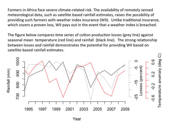
3.1. Association between Cotton Yield and Rainfall

Cotton in Zambia is almost exclusively rain-fed. It is to be expected, therefore, that when rain is low, losses are high. This is supported by Figure 1, which shows a convincing association between average losses over the 38 study locations and peak wet season rainfall (November–March rainfall) averaged over the domain shown (R² of 0.65, which is significant at the 95% level). Figure 1 suggests that temperature plays a secondary role (R² of 0.32), although the heavy losses in 2004 are associated with high temperatures as well as low rainfall. Note that Figure 1 includes only the post-1995 period, because prior to this, the loss data are based heavily on a yield stress model, and hence cannot be considered independent of the rainfall.

In spite of the generally strong association between losses and rainfall, there are clear discrepancies—with heavy losses experienced during some years of near normal rainfall. These may be explained by the wider social context of agriculture in Zambia. As well as rainfall variability, cotton production is affected by a multitude of economic factors. It is notable that around 2002, the Zambian Kwacha started to appreciate against the US Dollar, placing the export sector under increasing pressure. In response to the failing export market, in 2006, one of the largest cotton ginning companies, NWK-Agri-Services announced a 30% reduction in the price it would pay, resulting in a 40% drop in area planted during the 2007 season [43]. It is possible that price pressures or other socio-economic factors, rather than rainfall deficit, explain the magnitude of the fall in production during the 2006 and 2007 seasons. This wider context may also, in part explain the variability in cotton production outcomes since 2002.

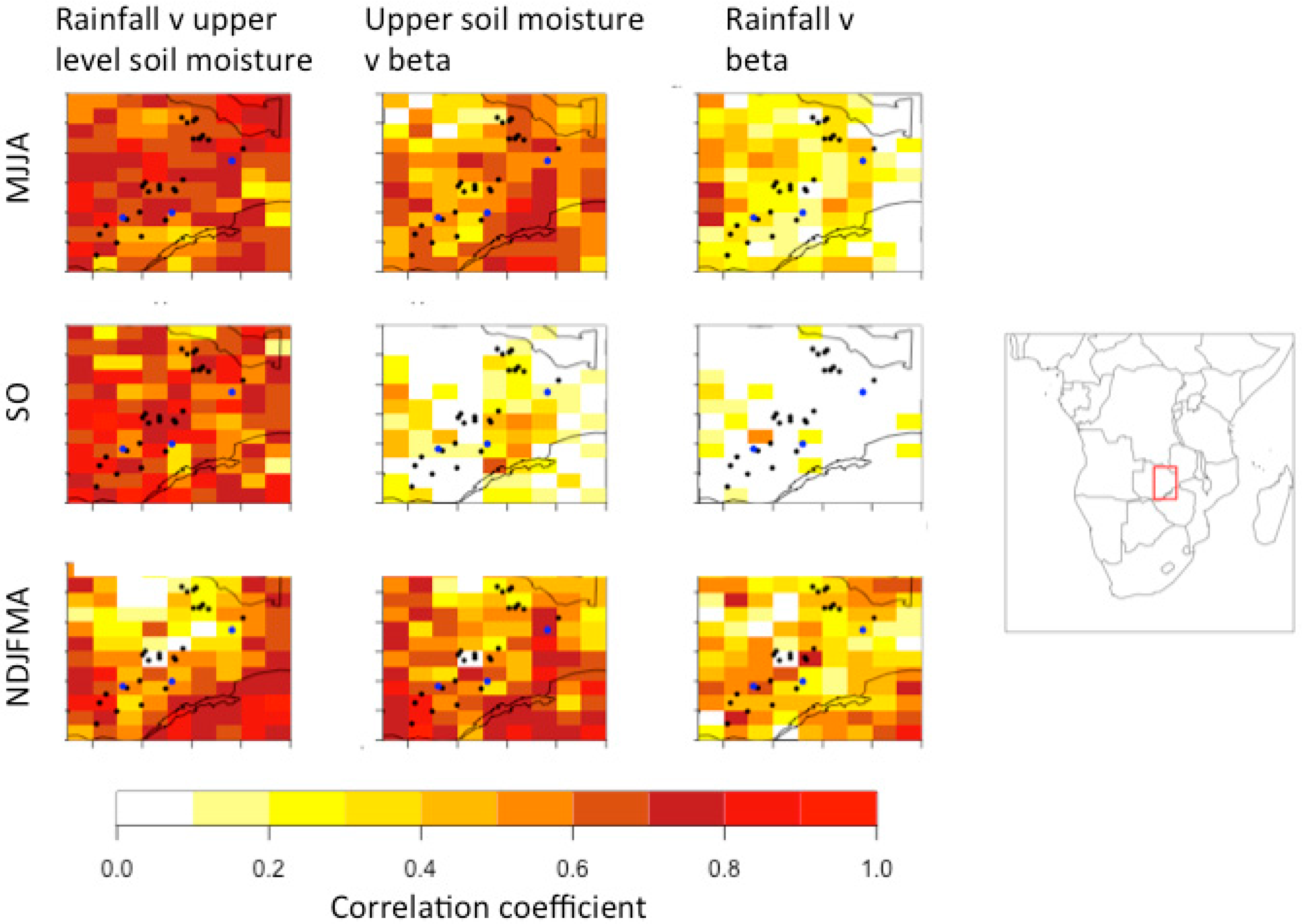
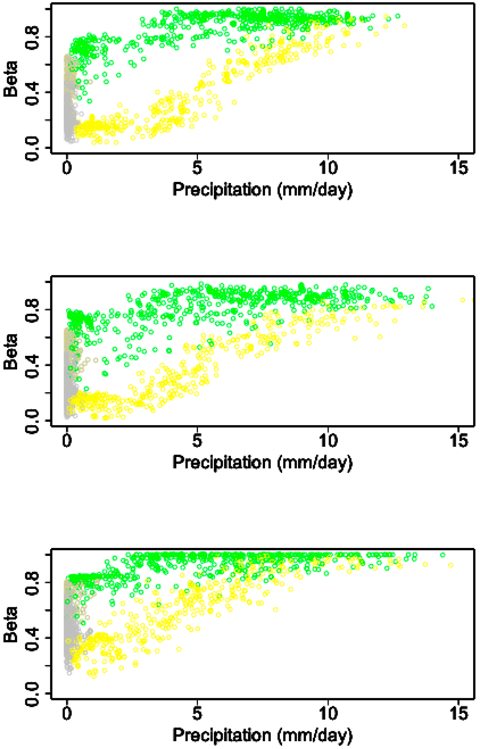
3.2. The Association between Rainfall and Soil Moisture

Zambia’s economic troubles exacerbate the population’s vulnerability to climate variability, particularly to drought. Robust WII could mitigate some of these risks, especially if it can be implemented at a large scale. As was described in Section 1, the fair implementation of drought WII requires a clear connection between rainfall and root zone soil moisture, i.e., a consistent progression from meteorological to agricultural drought. The progression from rainfall deficit to agricultural drought is illustrated by Figure 2, which shows the correlations between rainfall, upper level soil moisture and beta, for JULES driven with a single ensemble realization of rainfall. Correlation coefficients are calculated for inter-annual variability in variables of interest for the cool dry season (May–August), the hot dry season (September–October) and the rainy season (November–April). The time span over which the correlations are calculated is 1995–2010, which means that correlations over ~0.5 can be considered significant at the 95% level. The correlation between rainfall and upper level soil moisture (left column) relates to the infiltration of rainfall into the top layer of soil. The correlation between upper level soil moisture and beta (middle column) relates to percolation of water from the top layer of soil to the root zone. The correlation between rainfall and beta (right column) illustrates the ensuing link between rainfall and moisture availability to plants.

During the dry seasons, in May–August and September–October, the correlation between upper level soil moisture and rainfall is high because the top layer of soil is unsaturated. The correlations between top level soil moisture and beta are generally insignificant, and hence the correlations between beta and rainfall are low. During the rainy season (November–April), the correlation between upper layer soil moisture and beta is higher than in the dry season and this results in a closer link between total seasonal rainfall and mean beta. It is clear that the correlation between upper level soil moisture and beta varies spatially, reflecting heterogeneity in both climate and soil type. The variability illustrated in the maps of the correlation between beta and rainfall (bottom row) highlights the need to adjust WII indices spatially, and indeed to consider carefully which regions can be insured fairly using indices based on cumulative rainfall.

Figure 3 shows the seasonal cycles in correlation between rainfall and beta for the three study locations highlighted as blue circles on Figure 2, namely Chikanta (26°E; 16.4°S), Magoye (27.6°E; −16.0°S), and Makafu (28.8°E; 14.3°S). The plots show both the mean correlation for all ensemble members and the correlations for individual ensemble time series. Correlations are calculated for interannual time series for each month, over the same period as for Figure 2. The correlations are highest at the peak of the rainy season (November–January) and lowest in the middle of the dry season (June–July) for all three localities. There are, however, differences, reflecting spatial heterogeneity in both climate and land-surface properties. In particular, the stage of the season at which beta and rainfall become highly correlated varies, with correlations in the central locality (Magoye) remaining low until November, while the other localities exhibit strong correlations earlier in the season. The spread of ensemble members in Figure 3 suggests that uncertainty in observations of rainfall may obscure the link with beta, especially at the outset of the rainy season. More fundamentally, the error in rainfall estimates leads to significant uncertainty in the underlying relationship between rainfall and agricultural drought. This must be considered when using satellite based rainfall estimates, such as those described in Section 2 to design and price WII contracts.

The links between beta and rainfall for the three study locations are illustrated in Figure 4 and Figure 5, which relate beta to monthly/seasonal cumulative precipitation. Figure 4 shows beta plotted against monthly mean rainfall, distinguishing between the different parts of the season. The plots show how beta increases as the season progresses, reaching a maximum in January/February. For the central locality, beta increases more slowly than for the other locations, and as a result, the strong correlation between beta and rainfall persists through the season (Figure 3). For the other localities, beta reaches its maximum during the second half of the season, and as a result, the correlation between beta and rainfall drops markedly during January and February.

The relationship between rainfall and beta is explored further in Figure 5, which shows plots of beta versus cumulative precipitation during the peak of the rainy season (November–March). Broadly speaking, cumulative rainfall is proportional to beta, until beta approaches 1. The clarity of the link, however, varies from one locality to another. In particular, at Magoye (middle plot), there is more noise than at the other locations.

Figure 5 highlights 2004/5 which was chosen for the occurrence of losses at all three localities (15%, 24%, and 20% at Chikanta, Magoye, and Makafu respectively). At Makufu, and to a lesser extent Magoye, during 2001 the beta for a given cumulative rainfall was somewhat lower than usual, implying that the agricultural drought experienced was more severe than would be expected for the rainfall that occurred. For all three localities, the variability in beta explained by cumulative rainfall was greater when multiple ensembles for the same year are considered, than when multiple years for a single ensemble realization are considered. Thus, the large ensemble range of rainfall in some years does not translate to a large range in beta. In other words, high observational uncertainty in rainfall does not necessarily imply equivalently high uncertainty in the severity of agricultural drought.

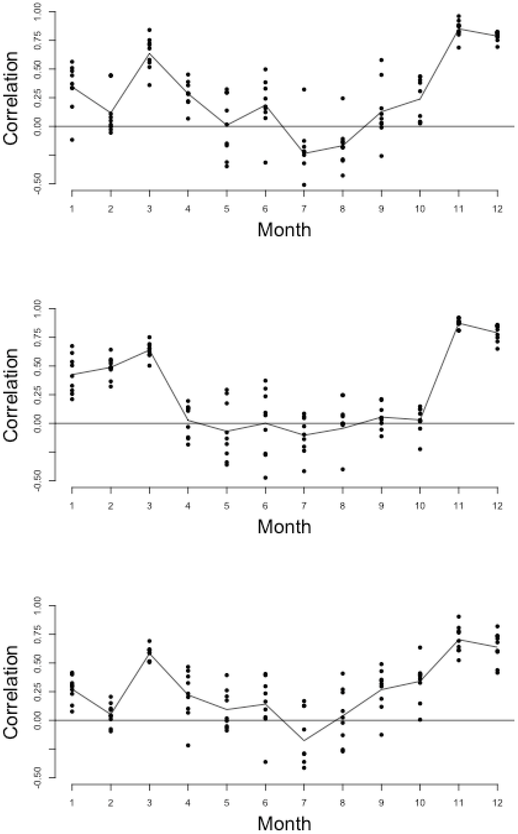
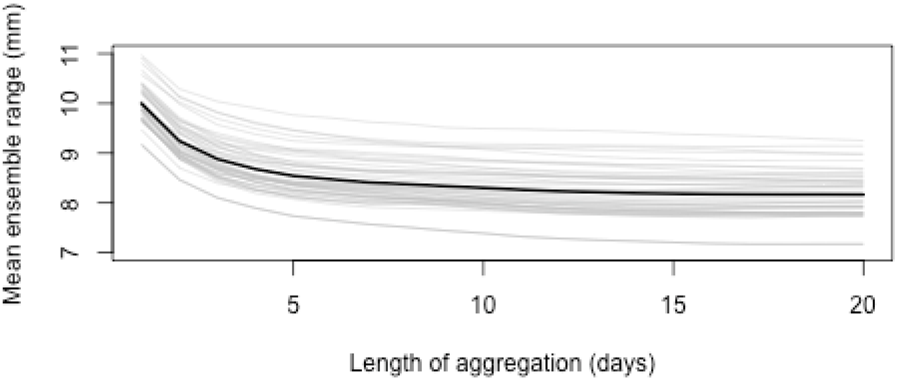
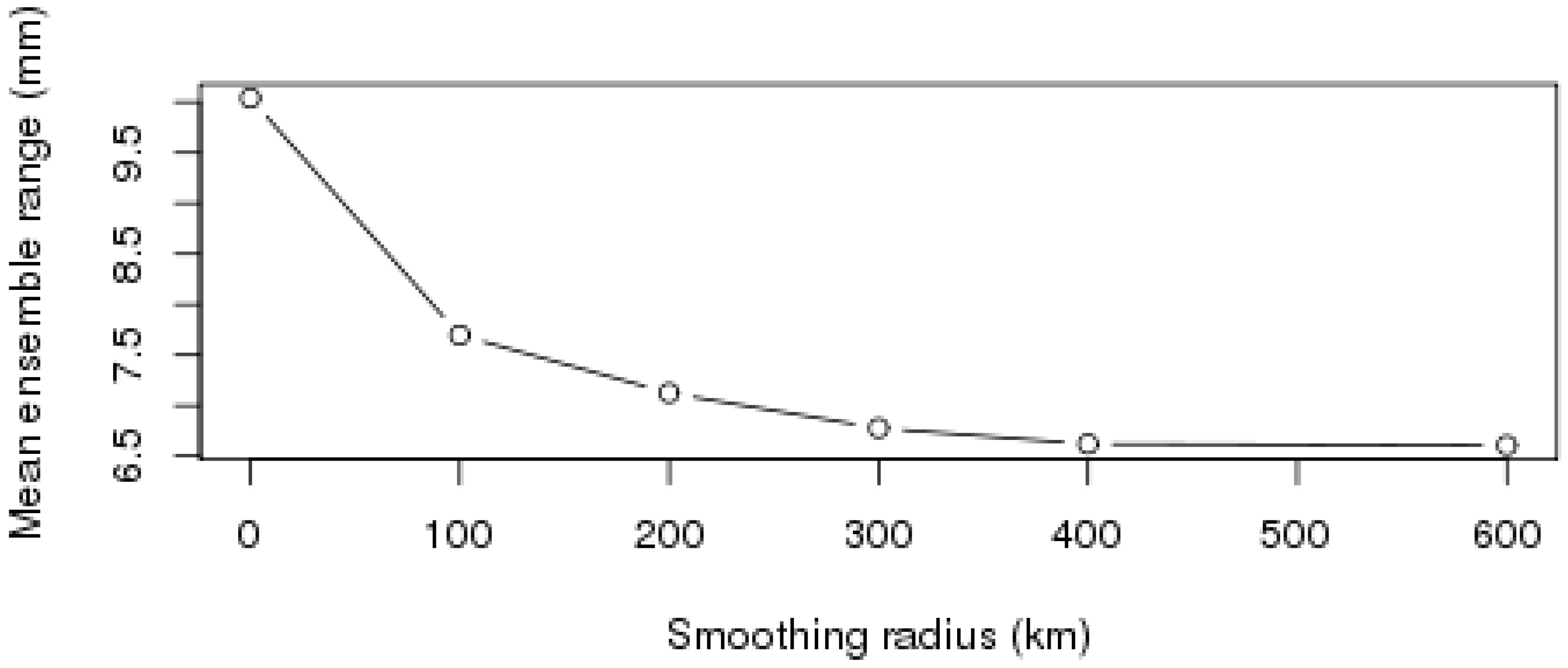
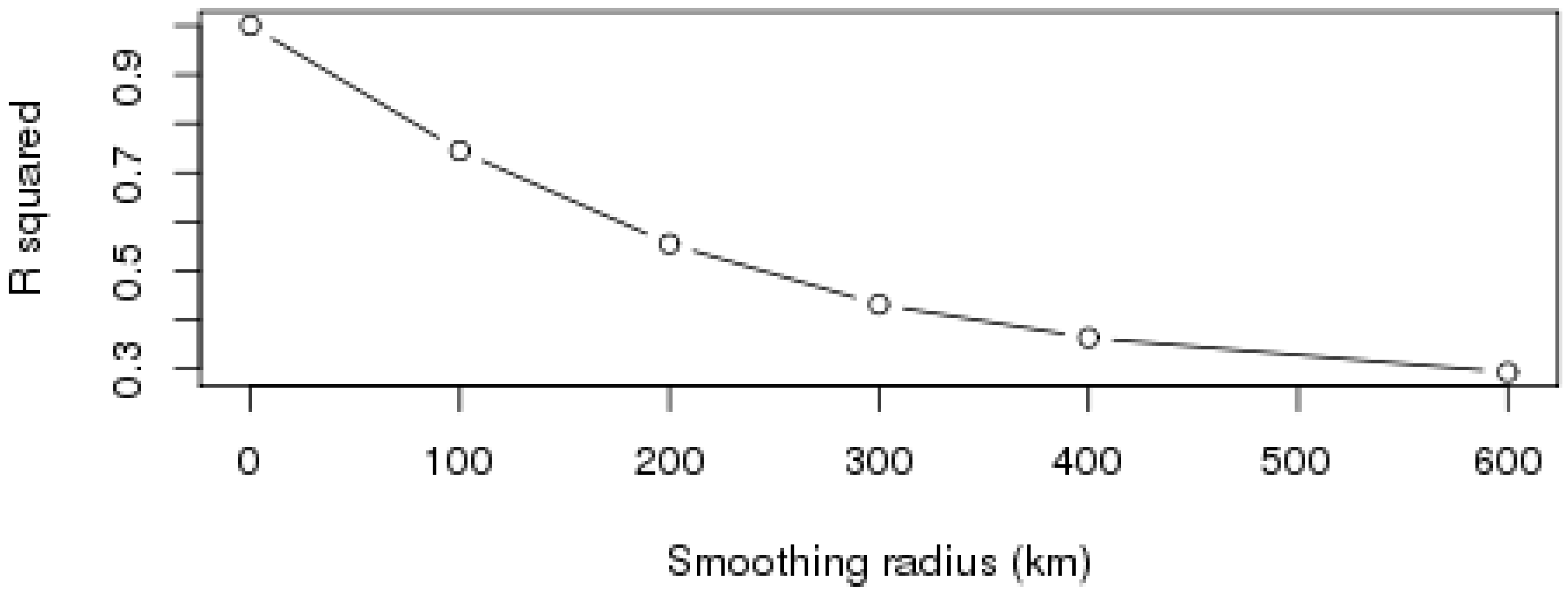
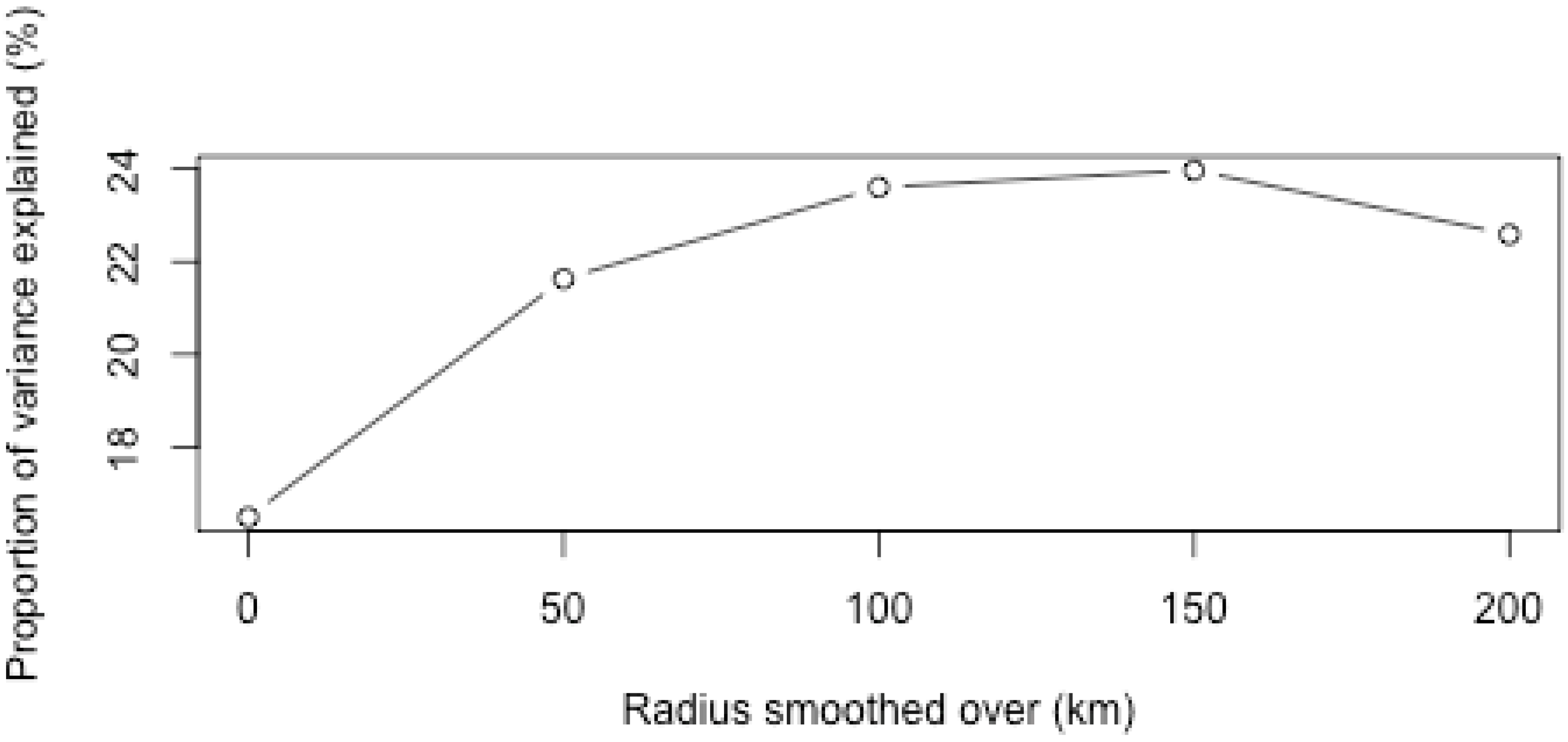
3.3. Aggregation of Remotely Sensed Rainfall in Time and Space

The findings described above highlight the need to design contracts that maximize skill and hence minimize basis risk when utilizing remotely sensed rainfall. Key to this is choosing an appropriate spatial and temporal scale for aggregation. Figure 6 shows how the mean range of the ensembles (bold black line), and hence the uncertainty in rainfall estimates, reduces as they are aggregated in time. It can be seen that there is significant variability in the magnitude of ensemble range from one locality to another, but that the shape of the curves is similar. At all localities, there is limited benefit from aggregating beyond five days. The example shown in Figure 6 is for January, but there were similar results for the whole rainy season.

Figure 7 illustrates an analogous effect when aggregating in space with clear reduction in ensemble range and hence uncertainty evident up to ~200 km. Beyond 400 km, there is little discernible improvement. When aggregating rainfall, however, the improvement in skill must be balanced against less accurate representation of local conditions. In other words, a 400 km × 400 km aerial mean rainfall estimate may be an accurate representation of rainfall over a 400 km × 400 km region, but a poor proxy for rainfall at any given point within it. This is illustrated by Figure 7, which shows the correlation between regionally averaged and local rainfall estimates (i.e., TAMSAT rainfall at a pixel), for regions ranging from 100 km × 100 km to 600 km × 600 km. It can be seen that there is a rapid drop off in correlation, so that beyond 300 km, values are bordering on statistically insignificant. This means that rainfall averaged over a 300 km × 300 km region is not representative of local rainfall.

The above analysis of aggregation in time and space provides useful information for index design. Figure 6 shows that the ensemble range is high when daily rainfall estimates are not aggregated in time. This means that at a daily time scale, TIR-based rainfall is highly uncertain. Indices based on statistics of individual days may, therefore, not be robust. An example of such an index would be n, where n is the number of days in a given period, for which rainfall is less than x mm. Conversely, indices based on cumulative rainfall are more robust. Spatially aggregating rainfall indices also reduces uncertainty (Figure 7), but it is necessary also to consider the effect of aggregation on the representation of local conditions.

Comparison between Figure 7 and Figure 8 can provide guidance as to the optimal spatial scale for aggregation. In Zambia, it has been found that indices based on rainfall averaged over 10 days closely match user experience of losses, as ascertained during farmer surveys carried out by Agrotosh Mookerjee. This is consistent with Figure 6, which shows that aggregating over periods greater than 5 days markedly increases skill. Figure 8, moreover, indicates rainfall averaged over a wide region would have higher skill, while still representing local conditions. It is important to recognize, moreover, that while this methodology is widely applicable, the optimal scale of aggregation is likely to vary from one region/season to another.

The first part of the discussion considered the progression from meteorological to agricultural drought, and the second part considered aggregation of rainfall estimates. These two factors are interlinked, and both must be considered when designing WII indices.

As well as being more reliably represented by the rainfall estimation methodology, cumulative seasonal precipitation is a better determinant of soil moisture deficit than monthly precipitation (Figure 4 and Figure 5). The link between soil moisture and rainfall also strengthens as these quantities are aggregated in space. This is confirmed by Figure 9, which shows how the percentage in variance in beta is explained by cumulative precipitation increases when the data are aggregated. It should be noted that although the effect is fairly small, it is coherent across the region (not shown). Because JULES does not account for lateral transfers of water (see Section 2), this effect can only be explained by the averaging out of extremes of rainfall and heterogeneities in the land surface. In reality, like any land surface hydrological variable, soil moisture is affected by aerially distributed rainfall. Figure 9 may therefore underestimate the effect of spatial aggregation on the link between rainfall and soil moisture.

These findings support the notion that an index based on spatially and temporally averaged remotely sensed rainfall can be a good proxy for agricultural drought as long as the aggregation is carried out at an appropriate scale. The optimal scale depends on spatial and temporal variability in the rainfall climate, the skill of estimation methodology, and the properties of the land-surface.

4. Discussion

WII is one of various instruments for reducing vulnerability to drought [14]. However, schemes that do not pay out during bad years, or pay out inappropriately during good years, may do more harm than good [44]. Essential to successful WII is an index that reflects the agricultural conditions experienced by the policy holder—i.e., low basis risk. Basis risk will be high if crop yield is strongly affected by factors that are not well correlated with the insured index. For example, if crops are insured on rainfall, but variability in yield is driven by pests and diseases, basis risk will be high. Low correlation between the rainfall index and field scale soil moisture will also increase basis risk.

In regions, such as Africa, where observational coverage is poor, inaccurate estimation of the insured index can worsen mismatch with agricultural losses. If ground-based observations are used, policy holders must live close enough to the station for the index to represent the meteorological conditions they are experiencing [45]. If remotely sensed data are used, the index must be skillfully represented by the dataset. In the case of remotely sensed rainfall, the skill with which an index is captured depends to a large extent on the degree of spatial and temporal aggregation. This is because aggregation in space and time, are generally increases accuracy [10].

Design of appropriate indices is especially challenging in regions that lack data for validation. In this study, errors in remotely sensed rainfall were assessed using a method designed to represent the inherent algorithmic uncertainty in the estimation process [17,18,19]. This approach has the advantage of not requiring dense coverage of ground-based data for evaluation. In the case study presented here, it was shown that, for Zambia, accuracy is significantly enhanced when rainfall is cumulated over 5 days or more, or over large spatial domains (>100 km) (Figure 6 and Figure 7). Skill resulting from spatial aggregation must, however, be balanced against loss of representativity of local conditions. For Zambia, rainfall is fairly homogenous, and Figure 8 shows that even up to ~150 km, aggregated rainfall skilfully captures local conditions. While these specific findings are applicable only to this case study, the methods of analysis are applicable anywhere.

In the absence of in situ root zone soil moisture measurements, the inherent link between rainfall and water stress on plants was assessed using a process-based land surface model. Figure 3, Figure 4 and Figure 5 show that at the peak of the rainy season, there is some correlation between plant water stress and temperature, but that this relationship varies considerably in both space and time. Such variability may explain some of the mismatches between rainfall and agricultural losses shown in Figure 1.

Over the last few years, several pilot WII schemes have been successfully implemented for cotton in southern Zambia, based on TAMSAT rainfall data. As such schemes are extended within Zambia and beyond, it is critical that insured indices continue to be rigorously evaluated. This study has presented a suite of methods that can be used for this purpose–even in the absence of dense networks of station observations.

5. Conclusions

• In Zambia, cotton production losses are associated with rainfall variability and specifically, total seasonal rainfall amount.
• There is a significant relationship between meteorological and agricultural drought on all spatial scales and throughout southern, central, and eastern Zambia.
• The high skill of satellite based rainfall estimates in the region opens up the possibility of expanding drought WII to a national level, provided that indices are carefully chosen to be skillfully reproduced by the satellite estimation methodology, representative of local conditions, and strongly linked to variability in soil moisture.

References

1. Boyd, E.; Cornforth, R.J.; Lamb, P.J.; Tarhule, A.; Lélé, M.I.; Brouder, A. Building resilience to face recurring environmental crisis in African Sahel. Nat. Clim. Chang. 2013, 3, 631–638. [Google Scholar] [CrossRef]
2. Cornforth, R.J. Weathering drought in Africa. Appropr. Technol. 2013, 40, 26–28. [Google Scholar]
3. Tarnavsky, E.; Grimes, D.; Maidment, R.; Black, E.; Allan, R.P.; Stringer, M.; Chadwick, R.; Kayitakire, F. Extension of the TAMSAT satellite-based rainfall monitoring over Africa and from 1983 to Present. J. Appl. Meteorol. Climatol. 2014, 53, 2805–2822. [Google Scholar] [CrossRef]
4. Novella, N.S.; Thiaw, W.M. African rainfall climatology version 2 for famine early warning systems. J. Appl. Meteorol. Climatol. 2013, 52, 588–606. [Google Scholar] [CrossRef]
5. Funk, C.; Peterson, P.; Landsfeld, M.; Pedreros, D.; Verdin, J.; Shukla, S.; Husak, G.; Rowland, J.; Harrison, L.; Hoell, A.; et al. The climate hazards infrared precipitation with stations—A new environmental record for monitoring extremes. Sci. Data 2015, 2, 150066. [Google Scholar] [CrossRef] [PubMed]
6. Hegerl, G.C.; Black, E.; Allan, R.P.; Ingram, W.J.; Polson, D.; Trenberth, K.E.; Chadwick, R.S.; Arkin, P.A.; Sarojini, B.B.; Becker, A. Challenges in quantifying changes in the global water cycle. Bull. Am. Meteorol. Soc. 2014, 96, 1097–1115. [Google Scholar] [CrossRef]
7. Dinku, T.; Chidzambwa, S.; Ceccato, P.; Connor, S.J.; Ropelewski, C.F. Validation of high-resolution satellite rainfall products over complex terrain. Int. J. Remote Sens. 2008, 29, 4097–4110. [Google Scholar] [CrossRef]
8. Dinku, T.; Ceccato, P.; Grover-Kopec, E.; Lemma, M.; Connor, S.J.; Ropelewski, C.F. Validation of satellite rainfall products over East Africa’s complex topography. Int. J. Remote Sens. 2007, 28, 1503–1526. [Google Scholar] [CrossRef]
9. Dinku, T.; Ceccato, P.; Connor, S.J. Challenges of satellite rainfall estimation over mountainous and arid parts of east Africa. Int. J. Remote Sens. 2011, 32, 5965–5979. [Google Scholar] [CrossRef]
10. Maidment, R.I.; Grimes, D.I.F.; Allan, R.P.; Greatrex, H.; Rojas, O.; Leo, O. Evaluation of satellite-based and model re-analysis rainfall estimates for Uganda. Meteorol. Appl. 2013, 20, 308–317. [Google Scholar] [CrossRef]
11. Milford, J.R.; McDougall, V.D.; Dugdale, G. Rainfall estimation from cold cloud duration: Experience of the TAMSAT group in West Africa. In Validation Problems of Rainfall Estimation by Satellite in Intertropical Africa; ORSTROM: Niamey, Niger, 1994; pp. 13–29. [Google Scholar]
12. Dugdale, G.; McDougall, V.; Milford, J. Rainfall estimates in the Sahel from cold cloud statistics: Accuracy and limitations of operational systems. In Proceedings of the International Workshop, Niamey, Niger, 18–23 February 1991; pp. 65–74.
13. Waller, J.A.; Dance, S.L.; Lawless, A.S.; Nichols, N.K.; Eyre, J.R. Representativity error for temperature and humidity using the Met Office high-resolution model. Q. J. R. Meteorol. Soc. 2014, 140, 1189–1197. [Google Scholar] [CrossRef]
14. Hess, U.; Richter, K.; Stoppa, A. Weather risk management for agriculture and agri-business in developing countries. In Climate Risk and the Weather Market, financial Risk Management with Weather Hedges; Risk Books: London, UK, 2002. [Google Scholar]
15. Barnett, B.J.; Mahul, O. Weather index insurance for agriculture and rural areas in lower-income countries. Am. J. Agric. Econ. 2007, 89, 1241–1247. [Google Scholar] [CrossRef]
16. Brown, M.E.; Osgood, D.E.; Carriquiry, M.A. Science-based insurance. Nat. Geosci. 2011, 4, 213–214. [Google Scholar] [CrossRef]
17. Greatrex, H.; Grimes, D.; Wheeler, T. Advances in the stochastic modeling of satellite-derived rainfall estimates using a sparse calibration dataset. J. Hydrometeorol. 2014, 15, 1810–1831. [Google Scholar] [CrossRef]
18. Teo, C.-K.; Grimes, D.I.F. Stochastic modelling of rainfall from satellite data. J. Hydrol. 2007, 346, 33–50. [Google Scholar] [CrossRef]
19. Grimes, D.I.F. An ensemble approach to uncertainty estimation for satellite-based rainfall estimates. In Hydrological Modelling and the Water Cycle; Springer: Berlin, Germany, 2008; pp. 145–162. [Google Scholar]
20. Javaid, I. Application of insecticides on cotton in Zambia: Timing of spray applications. Int. J. Pest Manag. 1990, 36, 1–9. [Google Scholar] [CrossRef]
21. Jamali, S.; Seaquist, J.; Ardö, J.; Eklundh, L. Investigating temporal relationships between rainfall, soil moisture and MODIS-derived NDVI and EVI for six sites in Africa. In Proceedings of the 34th International Symposium on Remote Sensing of Environment, Sydney, Australia, 10–15 April 2011.
22. Seneviratne, S.I.; Corti, T.; Davin, E.L.; Hirschi, M.; Jaeger, E.B.; Lehner, I.; Orlowsky, B.; Teuling, A.J. Investigating soil moisture-climate interactions in a changing climate: A review. Earth-Sci. Rev. 2010, 99, 125–161. [Google Scholar] [CrossRef]
23. Reddy, K.R.; Hodges, H.F.; Reddy, V.R. Temperature effects on cotton fruit retention. Agron. J. 1992, 84, 26–30. [Google Scholar] [CrossRef]
24. Brown, P. Cotton Heat Stress; College of Agriculture and Life Sciences, University of Arizona: Tucson, AZ, USA, 2008. [Google Scholar]
25. Traore, B.; Corbeels, M.; van Wijk, M.T.; Rufino, M.C.; Giller, K.E. Effects of climate variability and climate change on crop production in southern Mali. Eur. J. Agron. 2013, 49, 115–125. [Google Scholar] [CrossRef]
26. Best, M.J.; Pryor, M.; Clark, D.B.; Rooney, G.G.; Essery, R.L.H.; Ménard, C.B.; Edwards, J.M.; Hendry, M. A.; Porson, A.; Gedney, N.; et al. The Joint UK Land Environment Simulator (JULES), model description–Part 1: Energy and water fluxes. Geosci. Model Dev. 2011, 4, 677–699. [Google Scholar] [CrossRef]
27. Clark, D.B.; Mercado, L.M.; Sitch, S.; Jones, C.D.; Gedney, N.; Best, M.J.; Pryor, M.; Rooney, G.G.; Essery, R.L.H.; Blyth, E.; et al. The Joint UK Land Environment Simulator (JULES), model description–Part 2: Carbon fluxes and vegetation dynamics. Geosci. Model Dev. 2011, 4, 701–722. [Google Scholar] [CrossRef]
28. Dumedah, G.; Walker, J.P. Intercomparison of the JULES and CABLE land surface models through assimilation of remotely sensed soil moisture in southeast Australia. Adv. Water Resour. 2014, 74, 231–244. [Google Scholar] [CrossRef]
29. Blyth, E.; Gash, J.; Lloyd, A.; Pryor, M.; Weedon, G.P.; Shuttleworth, J. Evaluating the JULES land surface model energy fluxes using FLUXNET data. J. Hydrometeorol. 2010, 11, 509–519. [Google Scholar] [CrossRef]
30. Essery, B.R.L.H. The impact of new land surface physics on the GCM simulation of climate and climate sensitivity. Clim. Dyn. 1999, 15, 183–203. [Google Scholar]
31. Van Genuchten, M.T.; Wierenga, P.J. Mass transfer studies in sorbing porous media I. Analytical solutions. Soil Sci. Soc. Am. J. 1976, 40, 473–480. [Google Scholar] [CrossRef]
32. Johannes Dolman, A.; Gregory, D. The parametrization of rainfall interception in GCMs. Q. J. R. Meteorol. Soc. 1992, 118, 455–467. [Google Scholar] [CrossRef]
33. Weedon, G.P.; Balsamo, G.; Bellouin, N.; Gomes, S.; Best, M.J.; Viterbo, P. The WFDEI meteorological forcing data set: Watch forcing data methodology applied to ERA-Interim reanalysis data. Water Resour. Res. 2014, 50, 7505–7514. [Google Scholar] [CrossRef]
34. Maidment, R.I.; Grimes, D.; Allan, R.P.; Tarnavsky, E.; Stringer, M.; Hewison, T.; Roebeling, R.; Black, E. The 30 year TAMSAT African Rainfall Climatology and Time series (TARCAT) data set. J. Geophys. Res. Atmos. 2014, 119, 10619–10644. [Google Scholar] [CrossRef]
35. Thorne, V.; Coakeley, P.; Grimes, D.; Dugdale, G. Comparison of TAMSAT and CPC rainfall estimates with raingauges, for southern Africa. Int. J. Remote Sens. 2001, 22, 1951–1974. [Google Scholar] [CrossRef]
36. Dugdale, G.; Milford, J.R. Rainfall estimation over the Sahel using METEOSAT Thermal Infrared data. In Proceedings of the ISLSCP Conference, Rome, Italy, 2–6 December 1985.
37. Huffman, G.J.; Adler, R.F.; Morrissey, M.M.; Bolvin, D.T.; Curtis, S.; Joyce, R.; McGavock, B.; Susskind, J. Global precipitation at one-degree daily resolution from multisatellite observations. J. Hydrometeorol. 2001, 2, 36–50. [Google Scholar] [CrossRef]
38. Todd, M.C.; Kidd, C.; Kniveton, D.; Bellerby, T.J. A combined satellite infrared and passive microwave technique for estimation of small-scale rainfall. J. Atmos. Ocean. Technol. 2001, 18, 742–755. [Google Scholar] [CrossRef]
39. Laurent, H.; Jobard, I.; Toma, A. Validation of satellite and ground-based estimates of precipitation over the Sahel. Atmos. Res. 1998, 47, 651–670. [Google Scholar] [CrossRef]
40. Tucker, M.R.; Sear, C.B. A comparison of Meteosat rainfall estimation techniques in Kenya. Meteorol. Appl. 2001, 8, 107–117. [Google Scholar] [CrossRef]
41. Chadwick, R.S.; Grimes, D.I.F.; Saunders, R.W.; Francis, P.N.; Blackmore, T.A. The TAMORA algorithm: Satellite rainfall estimates over West Africa using multi-spectral SEVIRI data. Adv. Geosci. 2010, 25, 3–9. [Google Scholar] [CrossRef]
42. Jobard, I.; Chopin, F.; Berges, J.C.; Roca, R. An intercomparison of 10-day satellite precipitation products during West African monsoon. Int. J. Remote Sens. 2011, 32, 2353–2376. [Google Scholar] [CrossRef]
43. Kalinda, T.; Bwalya, R. An assessment of the growth opportunities and constraints in Zambia’s cotton industry. Asian J. Bus. Stud. 2014, 6, 63–75. [Google Scholar]
44. Sarker, J.R. Weather index insurance for agriculture in Bangladesh: Significance of implementation and some challenges. Eur. J. Bus. Manag. 2013, 5, 74–79. [Google Scholar]
45. Norton, M.T.; Turvey, C.; Osgood, D. Quantifying spatial basis risk for weather index insurance. J. Risk Financ. 2012, 14, 20–34. [Google Scholar] [CrossRef]
Figure 1. Time series of total November-March rainfall (black), temperature anomaly (red) and mean yield losses (grey) at the 38 locations shown in Figure 2.
Remotesensing 08 00342 g001
Figure 2. Correlation between rainfall and upper level soil moisture (left); upper level soil moisture and beta (middle); rainfall and beta (right) for (from top to bottom) May–August, September–October, November–April. Black circles are the localities for which loss data are available; blue circles represent the locations shown in Figure 3, Figure 4 and Figure 5 (from west to east: Chikanta, Magoye, Makafu). The area encompassed in these plots is shown as a red box on the map of Africa, on the right. The rainfall in the figure is from an example TAMSAT ensemble member.
Remotesensing 08 00342 g002
Figure 3. Interannual correlation between monthly mean rainfall and monthly mean beta for (from top to bottom) Chikanta, Magoye, Makafu. The dots are for individual ensemble rainfall realizations and the black line is mean correlation.
Remotesensing 08 00342 g003
Figure 4. Precipitation versus the JULES beta parameter for (from top to bottom) Chikanta, Magoye, and Makafu for May–September (grey circles), October-December (yellow circles), and January–April (green circles).
Remotesensing 08 00342 g004
Figure 5. Cumulative precipitation (November to March) versus the JULES beta parameter for (from top to bottom) Chikanta, Magoye, and Makafu. The brown dots and lines highlight one year (May 2004) during which were severe agricultural losses in Zambia.
Remotesensing 08 00342 g005
Figure 6. Time length of aggregation plotted against the mean ensemble range for the pixel containing each of the localities shown in Figure 2. The pale grey lines relate to individual time series and the bold line is the mean.
Remotesensing 08 00342 g006
Figure 7. Mean ensemble range as a function of box size, for a box centered on 25°E 15°S.
Remotesensing 08 00342 g007
Figure 8. Correlation between rainfall at a point at 25°E 15°S and mean rainfall in a box surrounding the point (y-axis), plotted as a function of the length of the side of the box (x-axis).
Remotesensing 08 00342 g008
Figure 9. Box side length of region averaged over (smoothing radius), versus the percentage of variance in beta explained by total precipitation for January.
Remotesensing 08 00342 g009