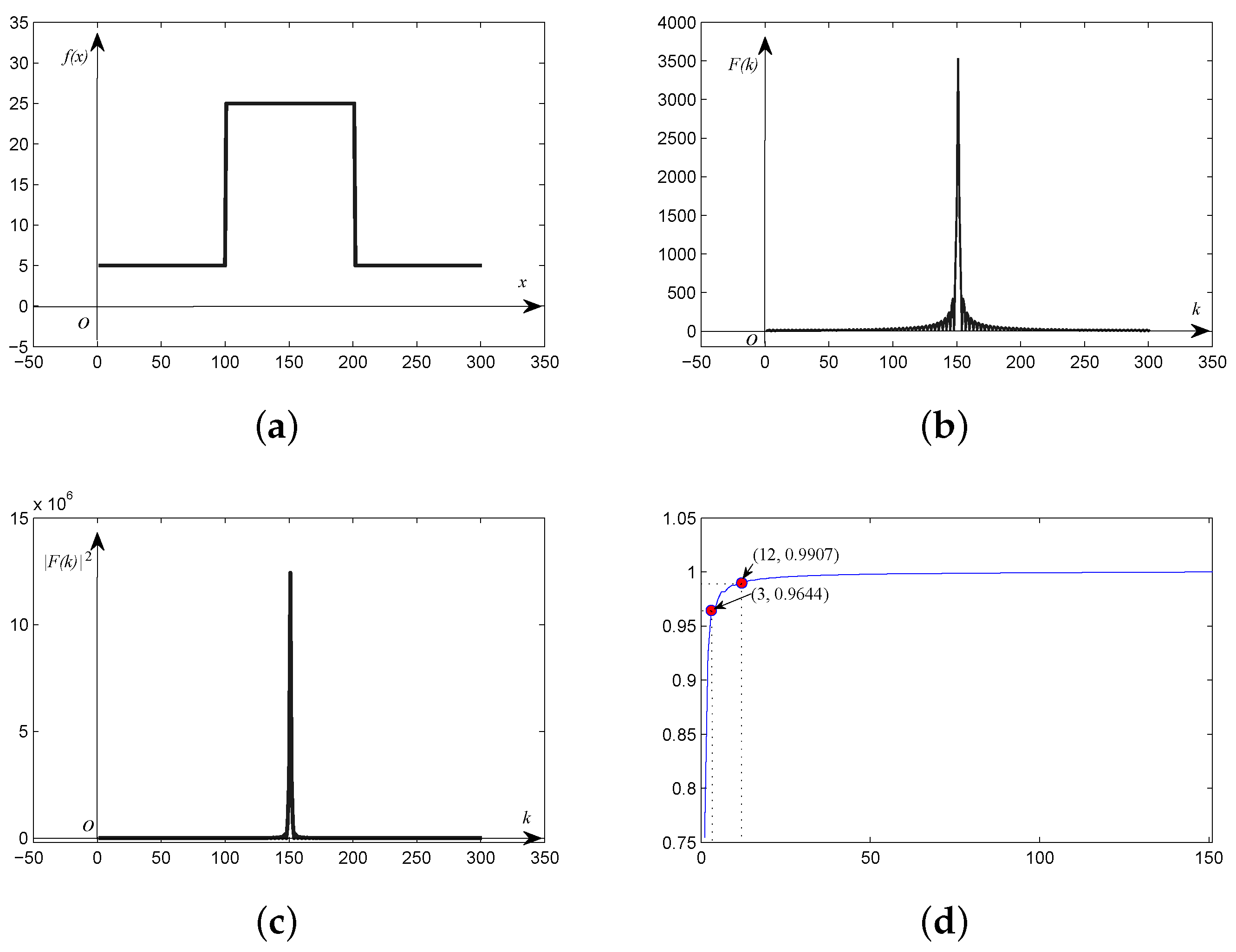
Figure 1.
(a) Square wave discrete signal; (b) frequency; and (c) power spectrum of the square wave signal; (d) ratio of frequency energy from the power spectrum.
Figure 1.
(a) Square wave discrete signal; (b) frequency; and (c) power spectrum of the square wave signal; (d) ratio of frequency energy from the power spectrum.
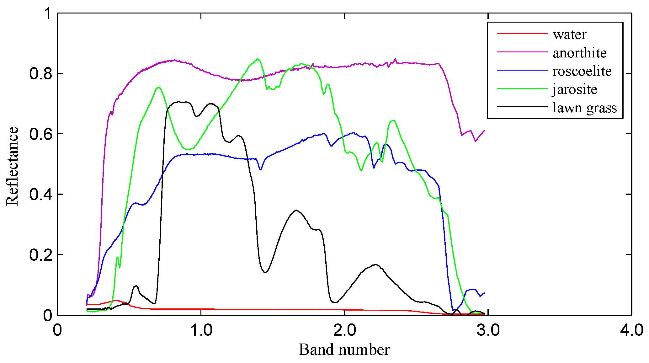
Figure 2.
Spectral signatures of water, anorthite, roscoelite, jarosite and lawn grass in the USGS spectral library.
Figure 2.
Spectral signatures of water, anorthite, roscoelite, jarosite and lawn grass in the USGS spectral library.
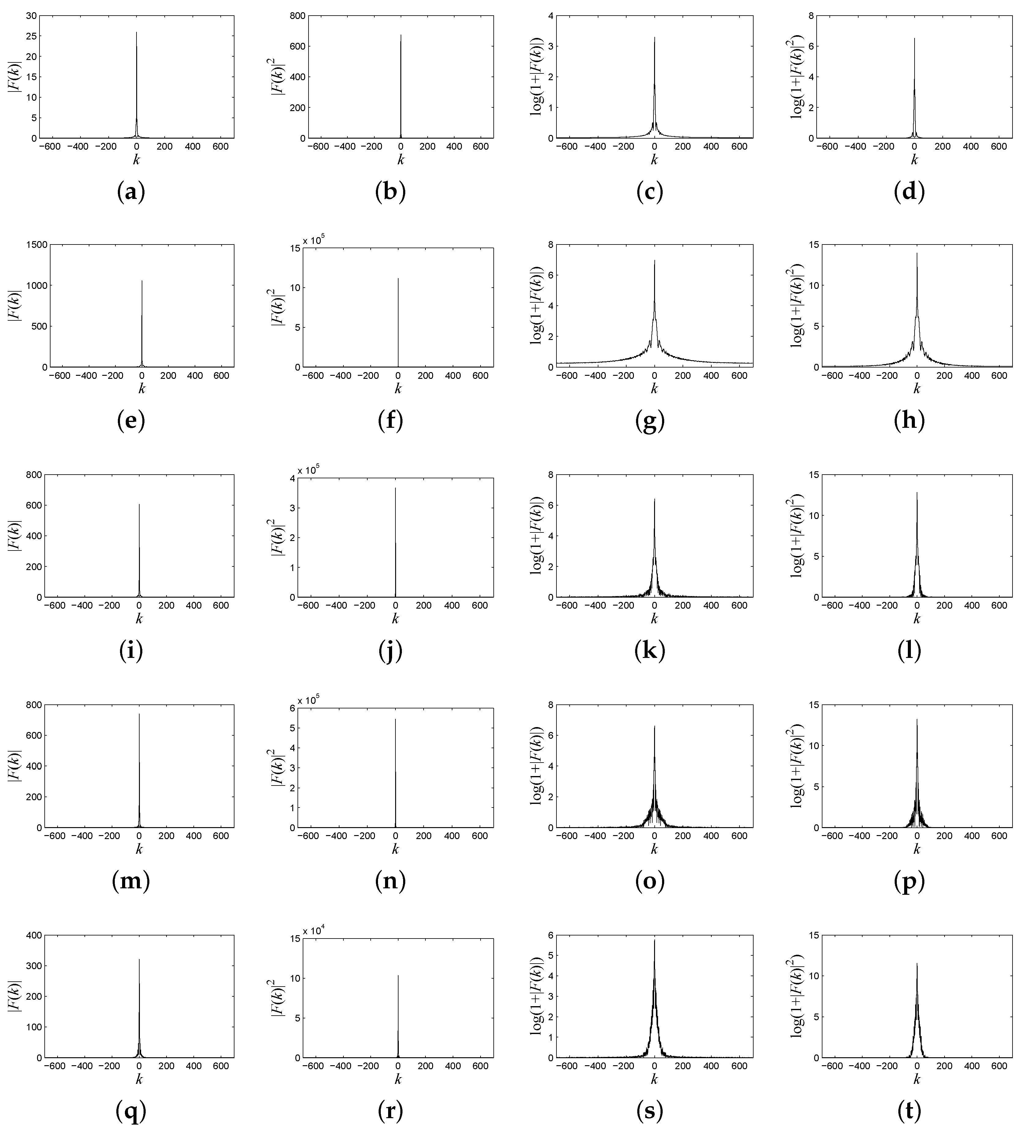
Figure 3.
(a) The frequency spectrum of the spectral signature of water; (b) the power spectrum of the spectral signature of water; (c) the logarithmic form of the frequency spectrum of the spectral signature of water; (d) the logarithmic form of the power spectrum of the spectral signature of water; (e) the frequency spectrum of the spectral signature of anorthite; (f) the power spectrum of the spectral signature of anorthite; (g) the logarithmic form of the frequency spectrum of the spectral signature of anorthite; (h) the logarithmic form of the power spectrum of the spectral signature of anorthite; (i) the frequency spectrum of the spectral signature of roscoelite; (j) the power spectrum of the spectral signature of roscoelite; (k) the logarithmic form of the frequency spectrum of the spectral signature of roscoelite; (l) the logarithmic form of the power spectrum of the spectral signature of roscoelite; (m) the frequency spectrum of the spectral signature of jarosite; (n) the power spectrum of the spectral signature of jarosite; (o) the logarithmic form of the frequency spectrum of the spectral signature of jarosite; (p) the logarithmic form of the power spectrum of the spectral signature of jarosite; (q) the frequency spectrum of the spectral signature of lawn grass; (r) the power spectrum of the spectral signature of lawn grass; (s) the logarithmic form of the frequency spectrum of the spectral signature of lawn grass; (t) the logarithmic form of the power spectrum of the spectral signature of lawn grass.
![Remotesensing 08 00344 g003]()
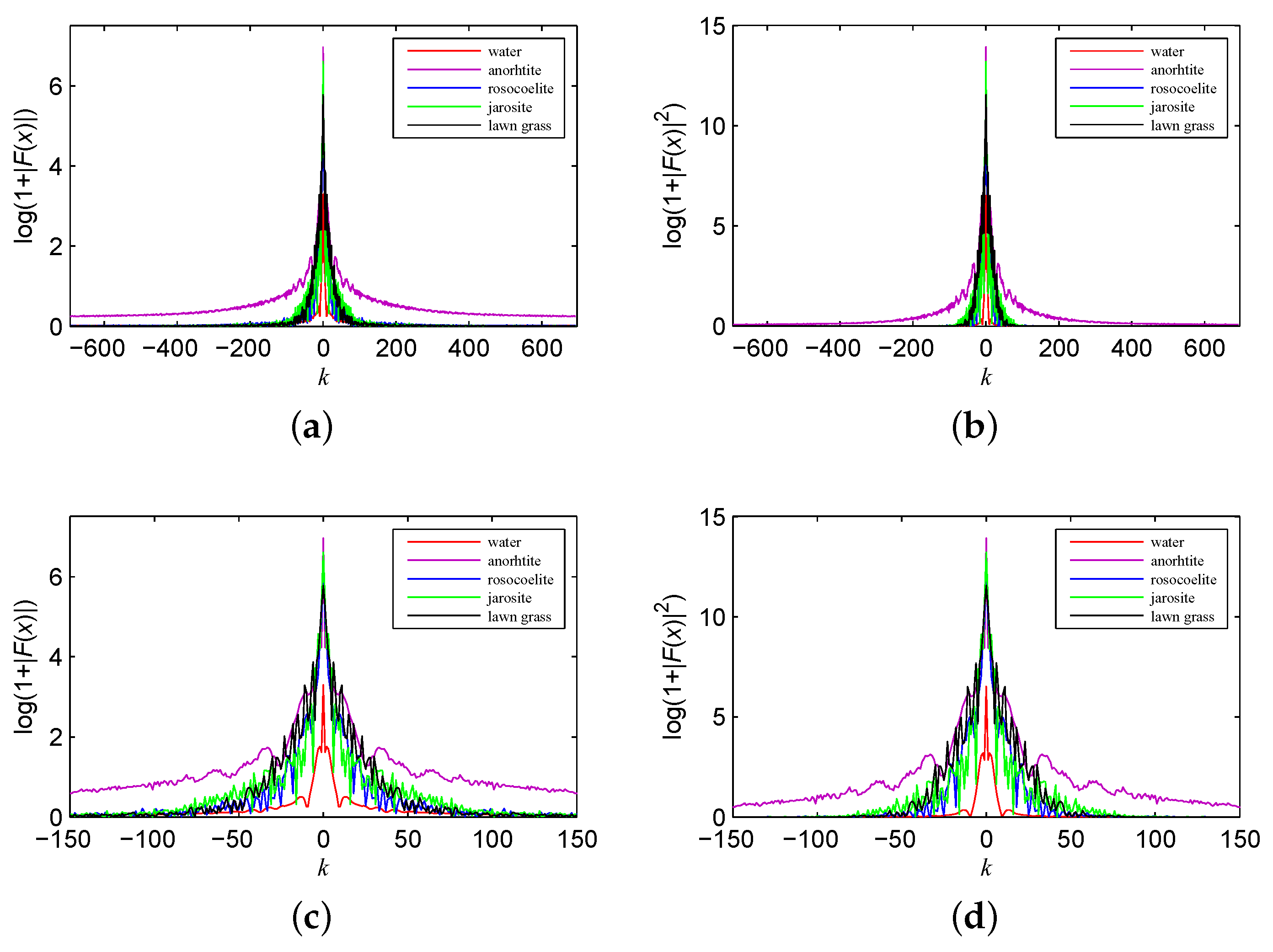
Figure 4.
Comparison of the (a) frequency and (b) power spectrum; details of the (c) frequency and (d) power spectrum.
Figure 4.
Comparison of the (a) frequency and (b) power spectrum; details of the (c) frequency and (d) power spectrum.
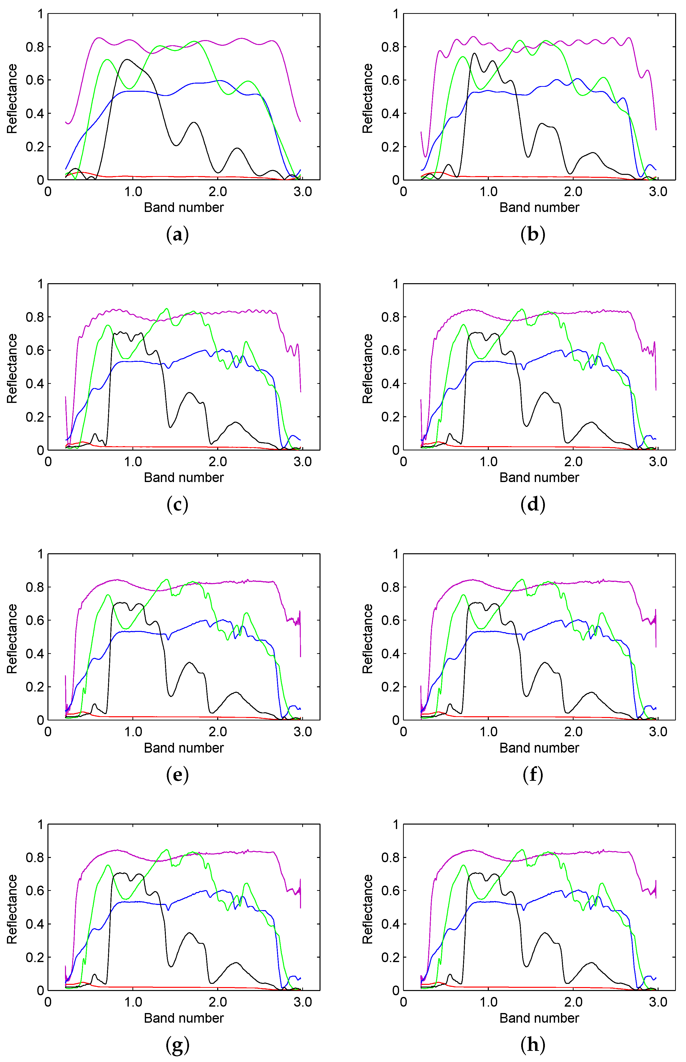
Figure 5.
Reconstruction results from (a) 1%; (b) 2%; (c) 5%; (d) 10%; (e) 20%; (f) 40%; (g) 60% and (h) 80% of the low frequency spectrum from the spectral signatures of water, anorthite, roscoelite, jarosite and lawn grass.
Figure 5.
Reconstruction results from (a) 1%; (b) 2%; (c) 5%; (d) 10%; (e) 20%; (f) 40%; (g) 60% and (h) 80% of the low frequency spectrum from the spectral signatures of water, anorthite, roscoelite, jarosite and lawn grass.
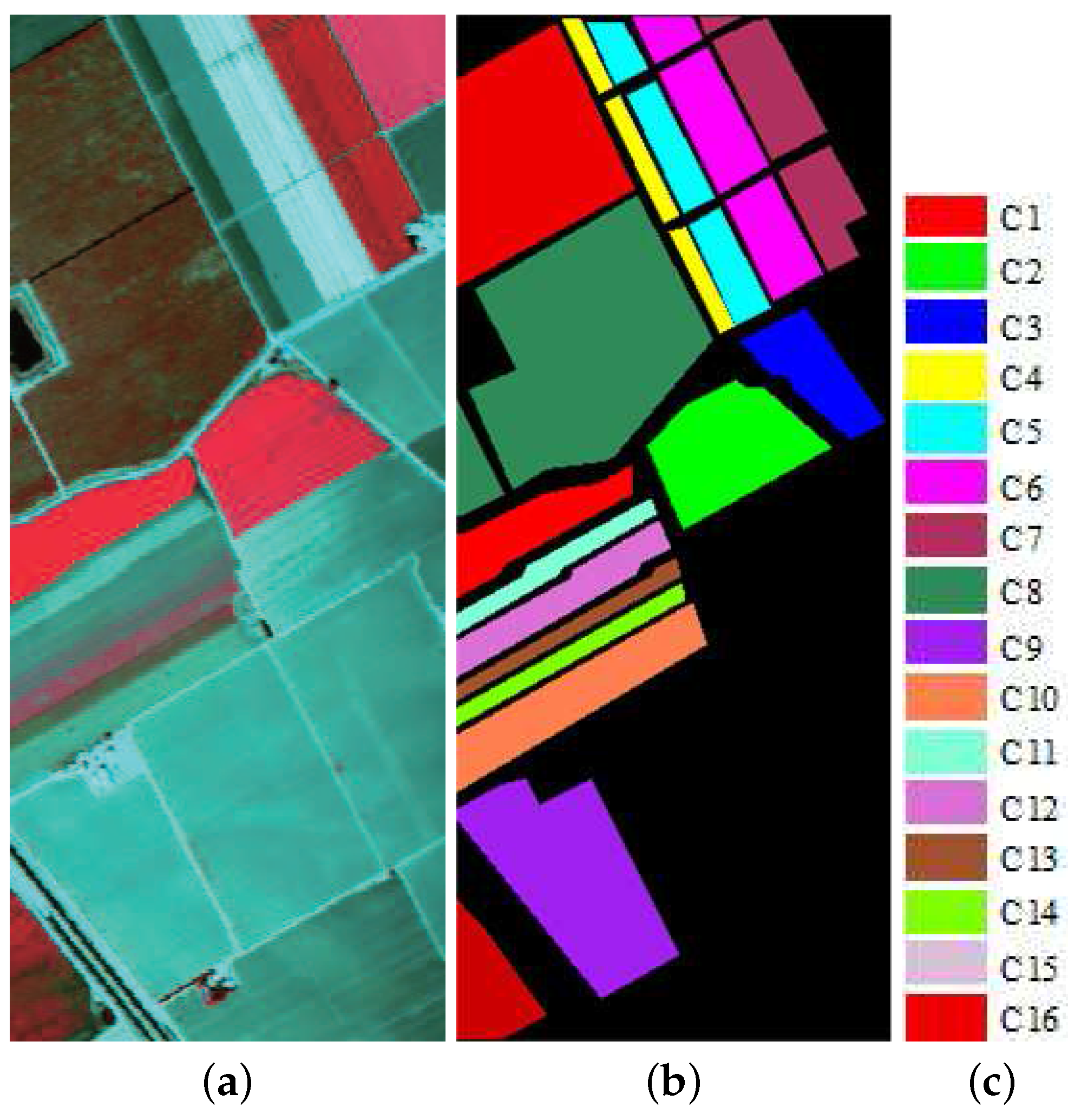
Figure 6.
(a) False color hyperspectral remote sensing image over the Salinas Valley (using Bands 68, 30 and 18); (b) ground truth of the labeled area with sixteen classes of land cover: Broccoli Green Weeds 1, Broccoli Green Weeds 2, fallow, fallow rough plow, fallow smooth, stubble, celery, grapes untrained, soil vineyard developed, corn senesced green weeds, romaine lettuce 4 wk, romaine lettuce 5 wk, romaine lettuce 6 wk, romaine lettuce 7 wk, vineyard untrained and vineyard vertical trellis. Note that wk here means week; (c) the legend of the classes for land cover of ground truth
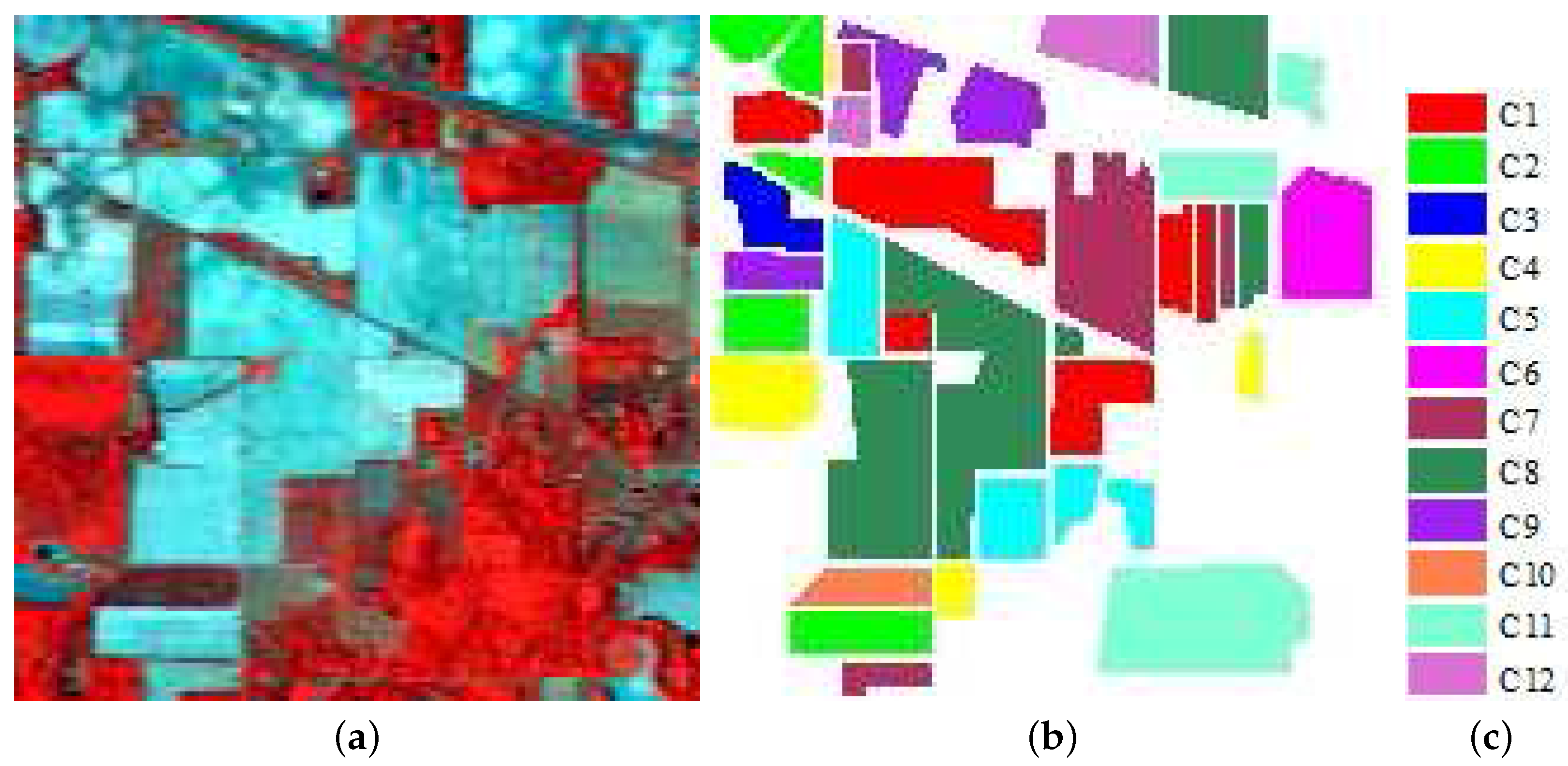
Figure 7.
(a) False color hyperspectral remote sensing image over the Indian Pines (using Bands 50, 27 and 17); (b) ground truth of the labeled area with twelve classes of land cover: corn-no till, corn-min till, corn, grass-pasture, grass-trees, hay-windrowed, soybean-no till, soybean-min till, soybean-clean, wheat, woods and buildings-grass-trees-drives; (c) the legend of the classes for land cover of ground truth
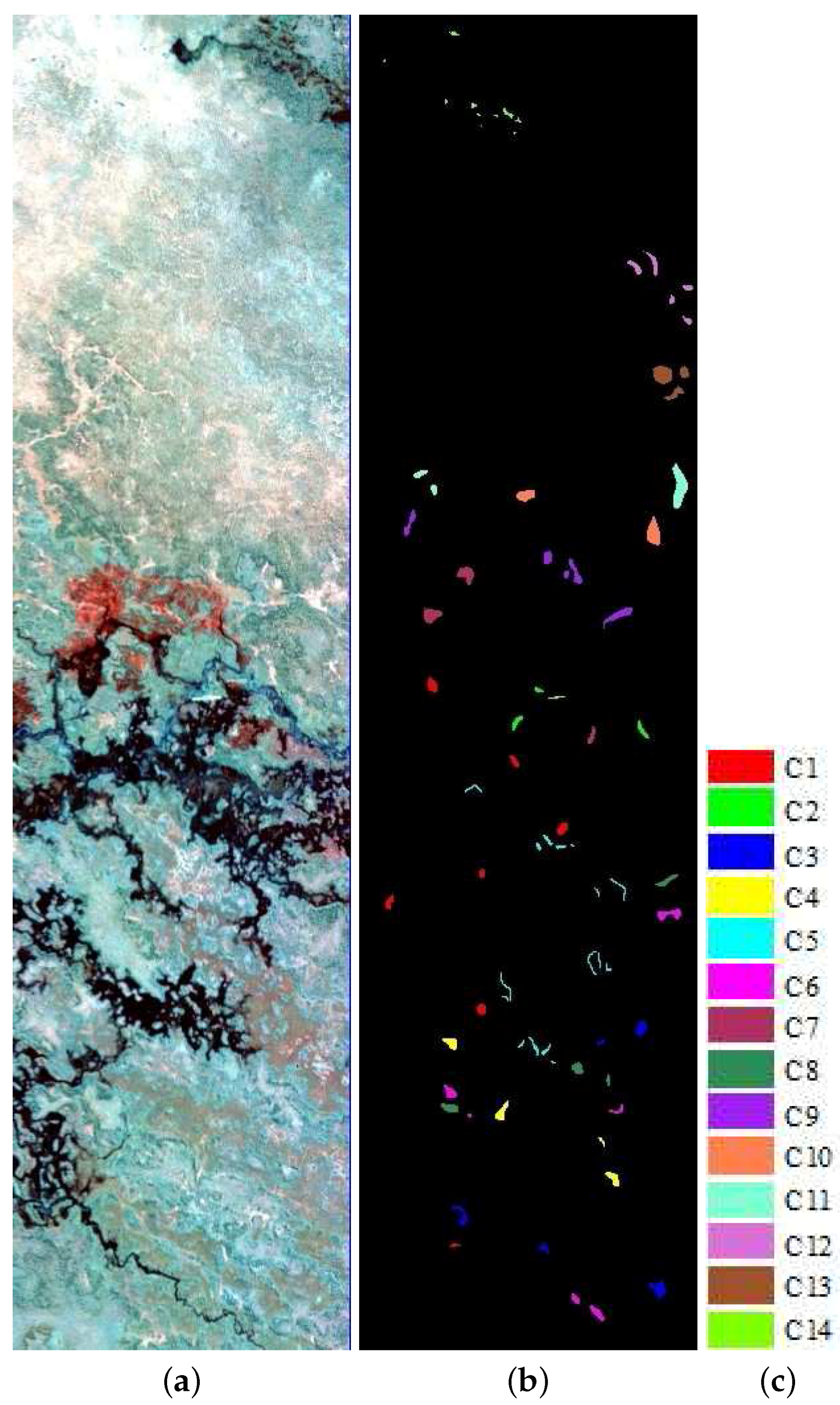
Figure 8.
(a) False color hyperspectral remote sensing image over Okavango Delta, Botswana (using Bands 149, 51 and 31); (b) ground truth of the labeled area with twelve classes of land cover: water, hippo grass, floodplain grasses 1, floodplain grasses 2, reeds 1, riparian, firescar 2, island interior, acacia woodlands, acacia shrublands, acacia grasslands, short mopane, mixed mopane and exposed soils; (c) the legend of the classes of land cover for ground truth
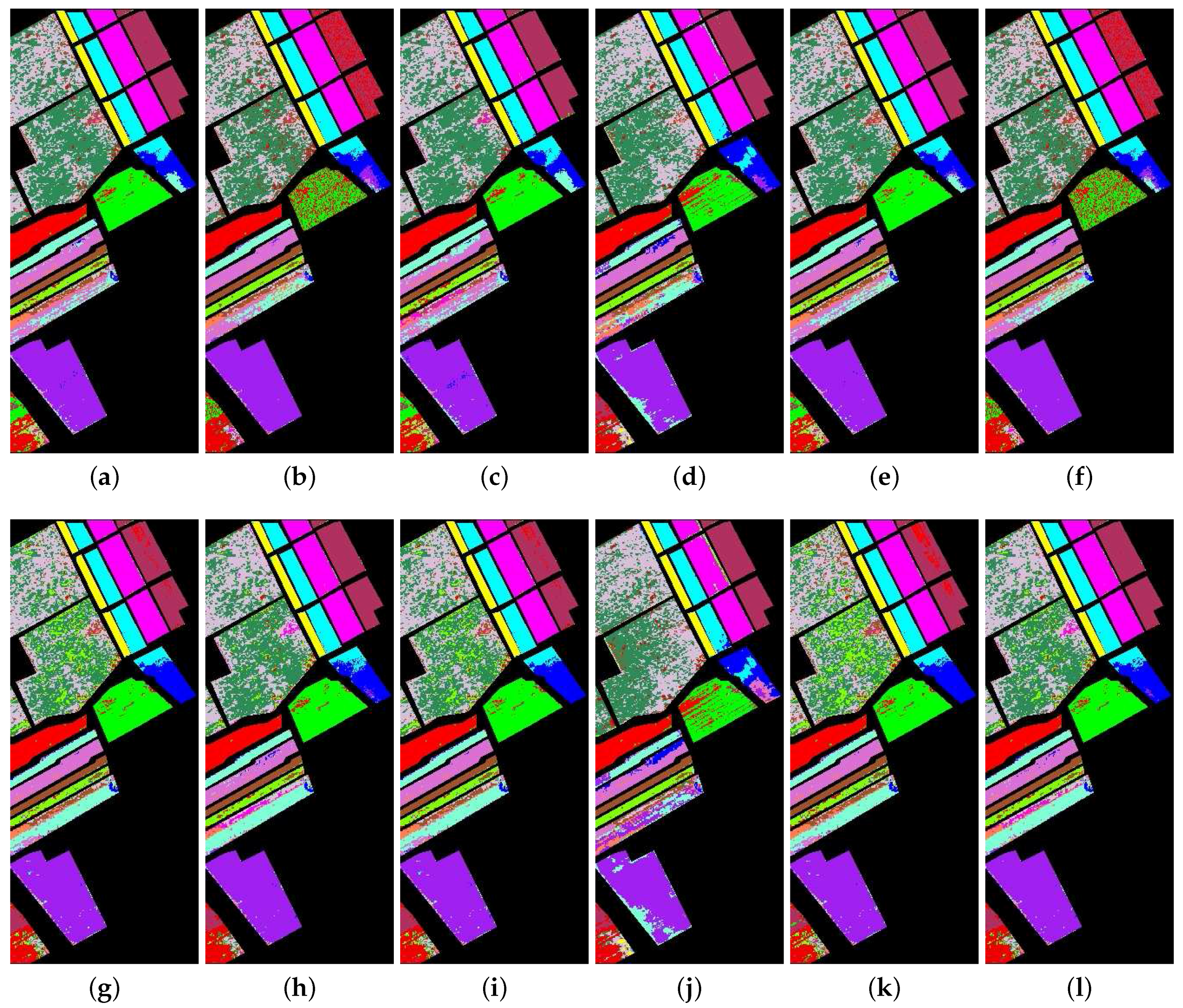
Figure 9.
The classification map from the hyperspectral data on Salinas Valley. The first row is the result from the SAM, SID, SCM, ED, NED, and SsS methods, respectively; the second row is the result from the F-SAM, F-SID, F-SCM, F-ED, F-NED and F-SsS methods, respectively. (a) SAM; (b) SID; (c) SCM; (d) ED; (e) NED; (f) SsS; (g) F-SAM; (h) F-SID; (i) F-SCM; (j) F-ED; (k) F-NED; (l) F-SsS.
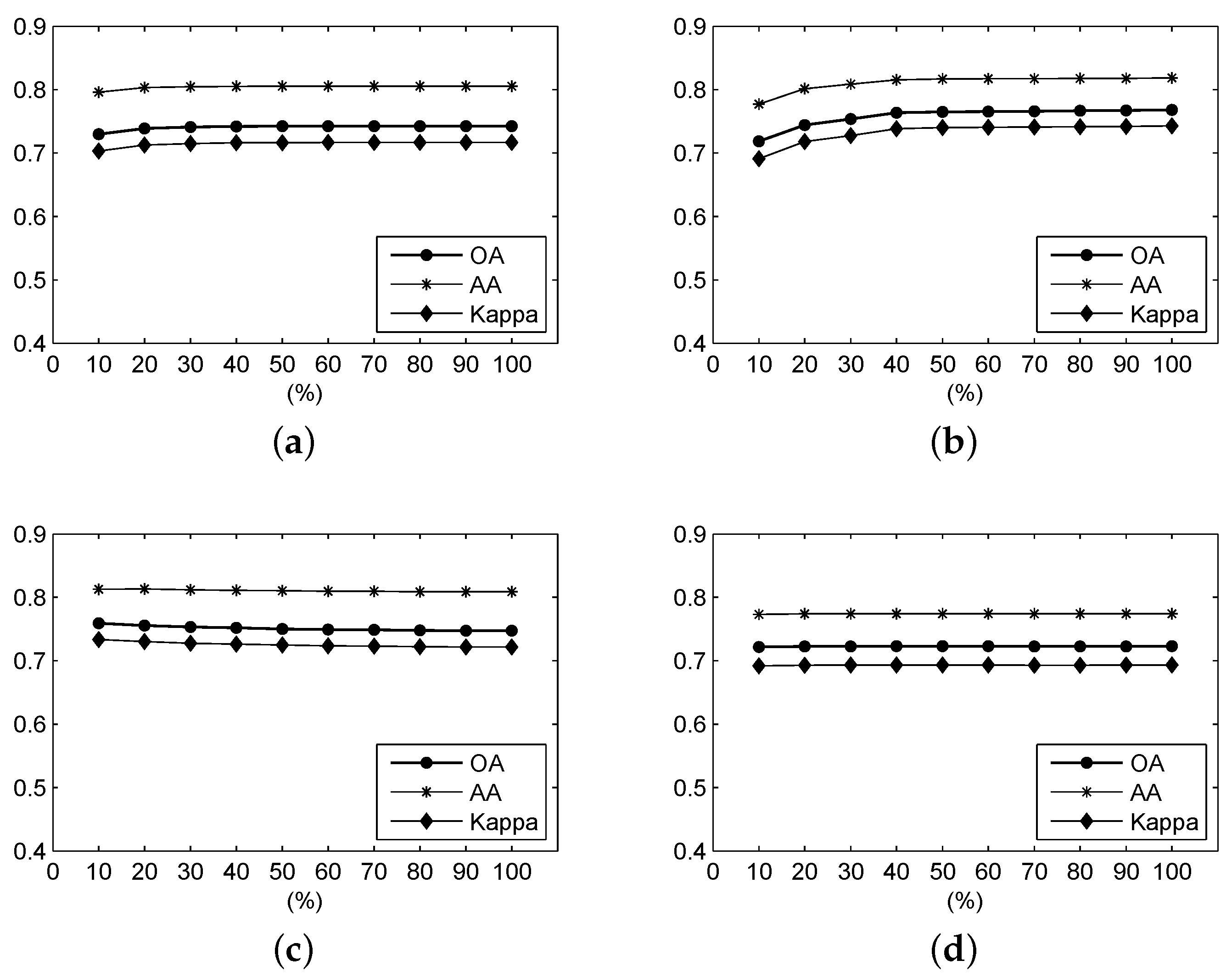
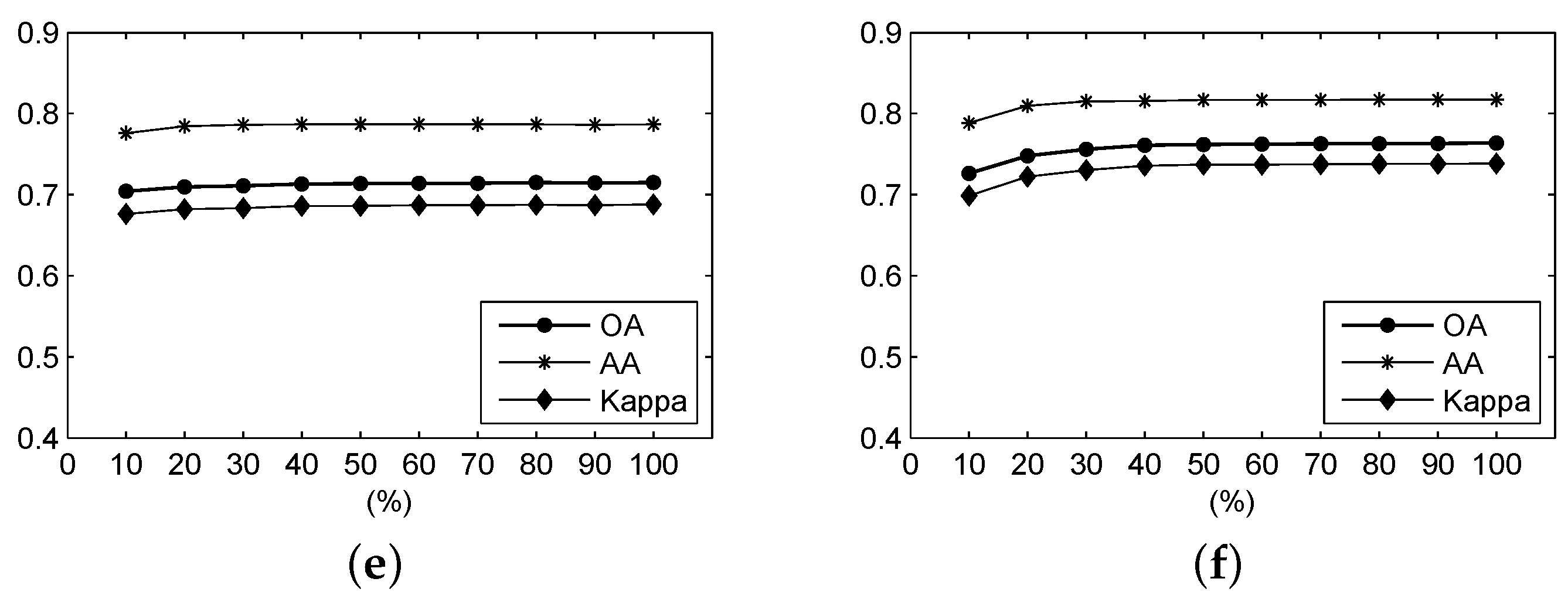
Figure 10.
For the Salinas Valley data, the OA, AA and Kappa coefficient of the classification result under different parameters using (a) F-SAM, (b) F-SID, (c) F-SCM, (d) F-ED, (e) F-NED, and (f) F-SsS.
Figure 10.
For the Salinas Valley data, the OA, AA and Kappa coefficient of the classification result under different parameters using (a) F-SAM, (b) F-SID, (c) F-SCM, (d) F-ED, (e) F-NED, and (f) F-SsS.
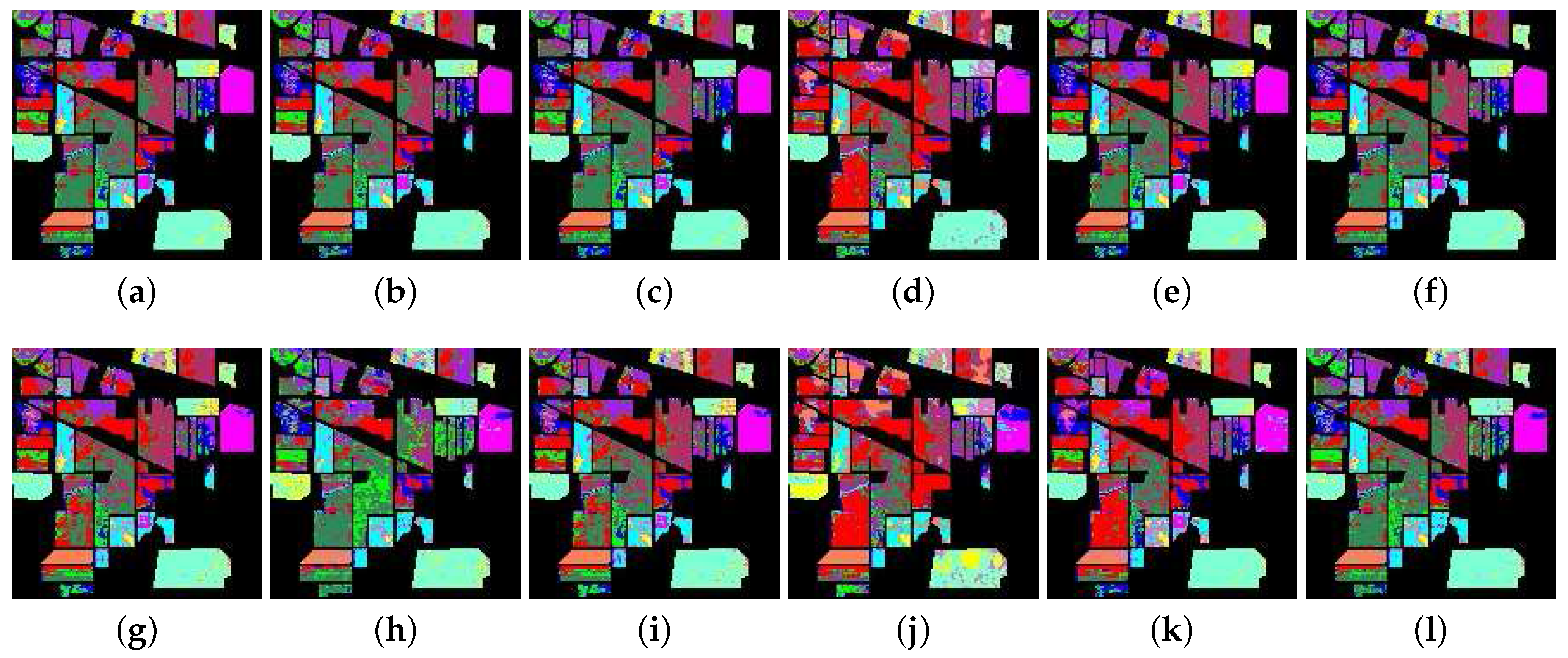
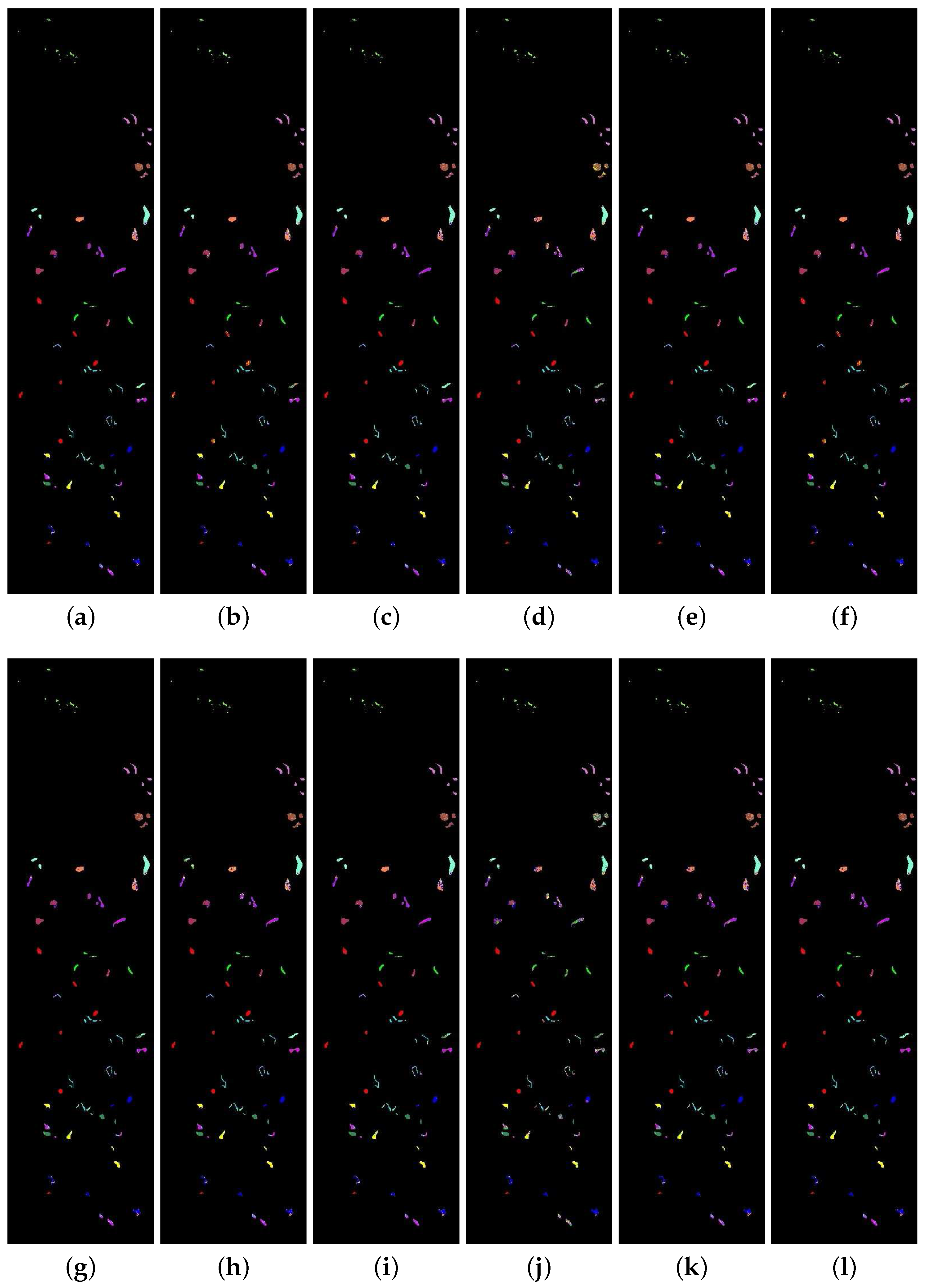
Figure 11.
The classification map from the hyperspectral data on Indian Pines. The first row is the result from the SAM, SID, SCM, ED, NED, and SsS methods, respectively; the second row is the result from the F-SAM, F-SID, F-SCM, F-ED, F-NED and F-SsS methods, respectively. (a) SAM; (b) SID; (c) SCM; (d) ED; (e) NED; (f) SsS; (g) F-SAM; (h) F-SID; (i) F-SCM; (j) F-ED; (k) F-NED; (l) F-SsS.
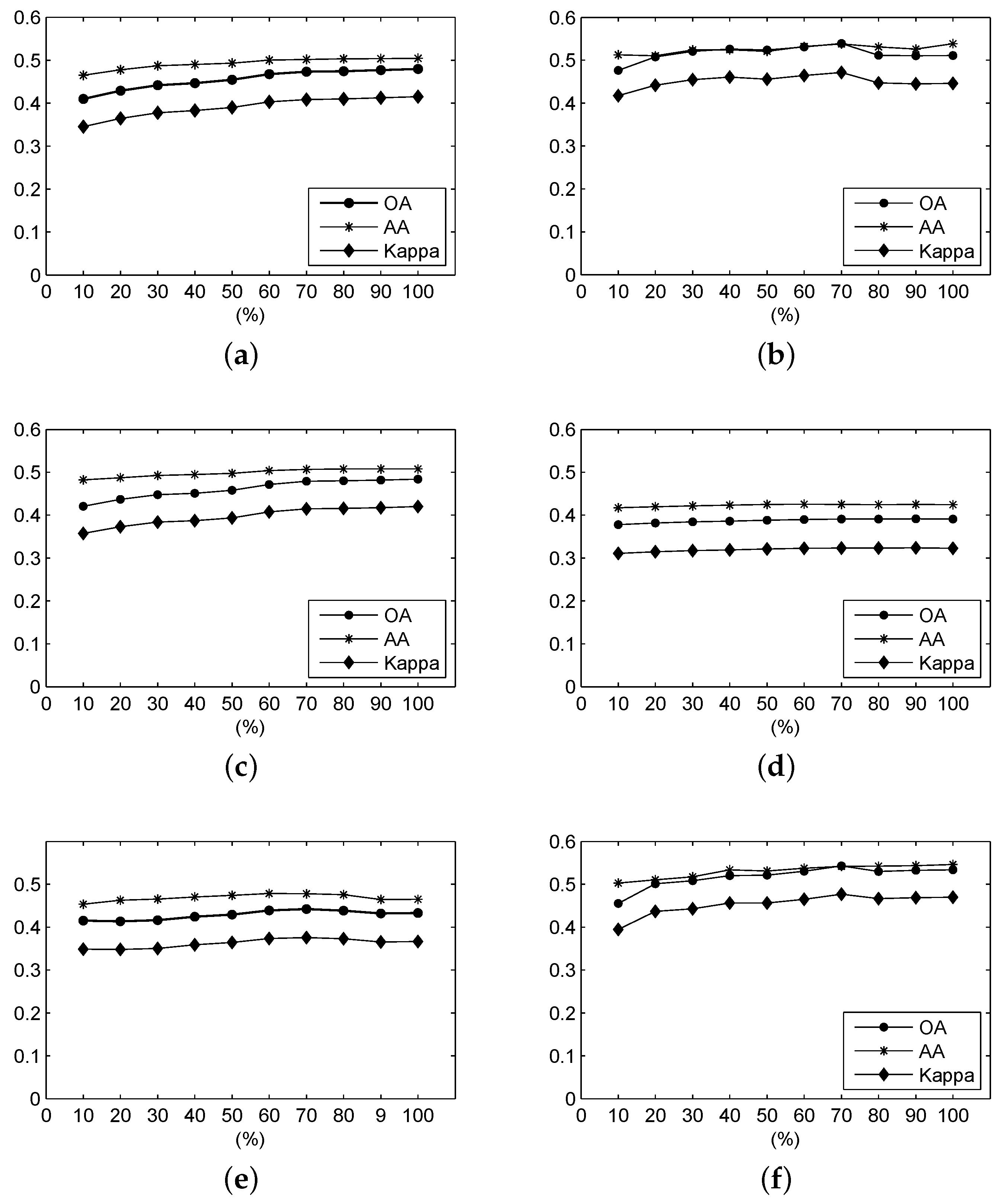
Figure 12.
For the Indian Pines data, the OA, AA and Kappa coefficient of the classification results under different parameters using (a) F-SAM; (b) F-SID; (c) F-SCM; (d) F-ED; (e) F-NED; and (f) F-SsS.
Figure 12.
For the Indian Pines data, the OA, AA and Kappa coefficient of the classification results under different parameters using (a) F-SAM; (b) F-SID; (c) F-SCM; (d) F-ED; (e) F-NED; and (f) F-SsS.
Figure 13.
The classification map from the hyperspectral data on Botswana. The first row is the result from the SAM, SID, SCM, ED, NED, and SsS methods, respectively; the second row is the result from the F-SAM, F-SID, F-SCM, F-ED, F-NED and F-SsS methods, respectively. (a) SAM; (b) SID; (c) SCM; (d) ED; (e) NED; (f) SsS; (g) F-SAM; (h) F-SID; (i) F-SCM; (j) F-ED; (k) F-NED; (l) F-SsS.
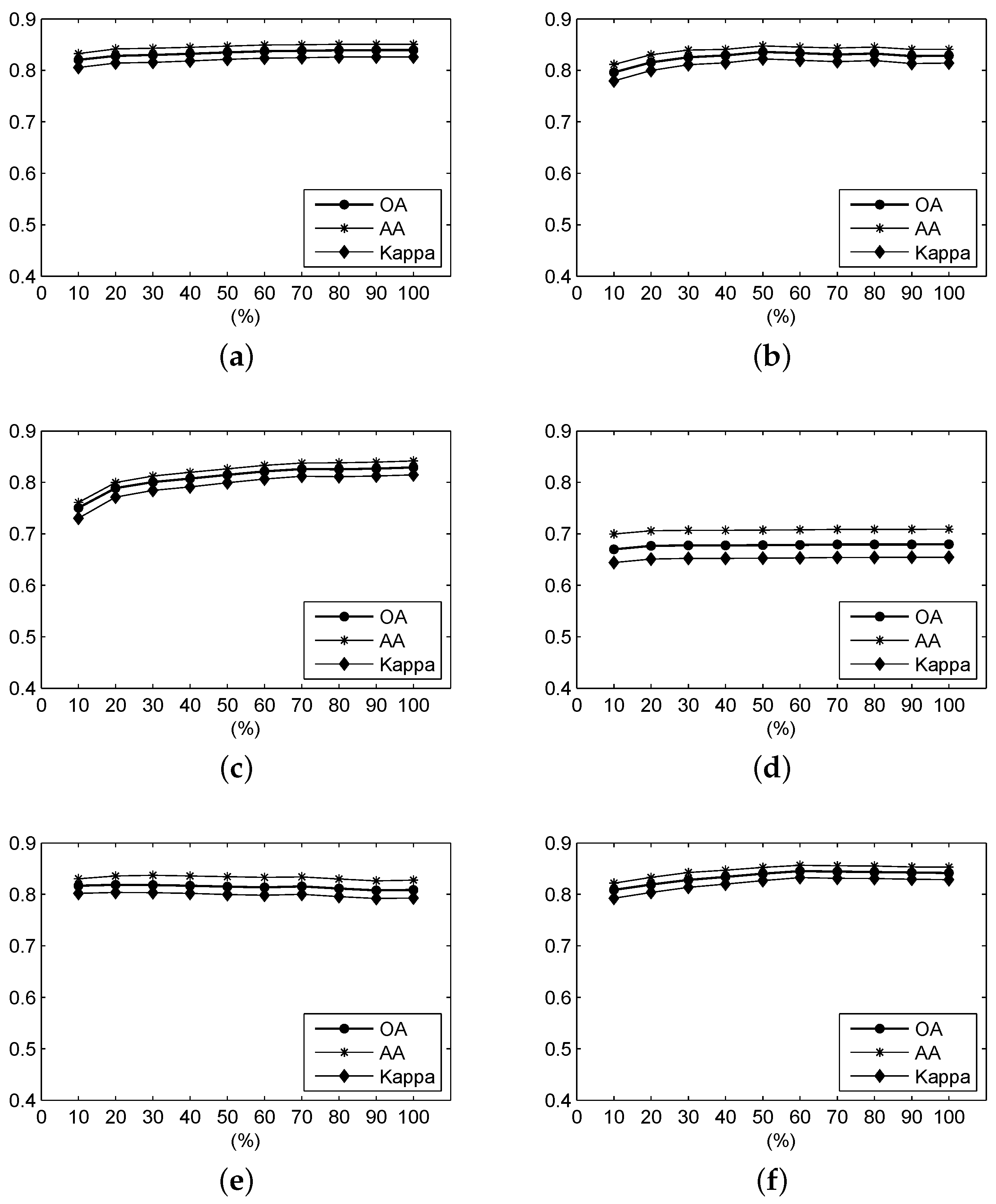
Figure 14.
For the Botswana data, the OA, AA and Kappa coefficient of the classification result under different parameters using (a) F-SAM; (b) F-SID; (c) F-SCM; (d) F-ED; (e) F-NED; and (f) F-SsS.
Figure 14.
For the Botswana data, the OA, AA and Kappa coefficient of the classification result under different parameters using (a) F-SAM; (b) F-SID; (c) F-SCM; (d) F-ED; (e) F-NED; and (f) F-SsS.
Table 1.
Ground truth classes for the Salinas Valley scene and their respective sample number.
Table 1.
Ground truth classes for the Salinas Valley scene and their respective sample number.
| Label | Class | Samples |
|---|
| C1 | Broccoli Green Weeds 1 | 2009 |
| C2 | Broccoli Green Weeds 2 | 3726 |
| C3 | Fallow | 1976 |
| C4 | Fallow rough plow | 1394 |
| C5 | Fallow smooth | 2678 |
| C6 | Stubble | 3959 |
| C7 | Celery | 3579 |
| C8 | Grapes untrained | 11,271 |
| C9 | Soil vineyard develop | 6203 |
| C10 | Corn senesced green weeds | 3278 |
| C11 | Romaine lettuce 4 wk | 1068 |
| C12 | Romaine lettuce 5 wk | 1927 |
| C13 | Romaine lettuce 6 wk | 916 |
| C14 | Romaine lettuce 7 wk | 1070 |
| C15 | Vineyard untrained | 7268 |
| C16 | Vineyard vertical trellis | 1807 |
| Total | | 54,129 |
Table 2.
Ground truth classes for the Indian Pines scene and their respective sample number.
Table 2.
Ground truth classes for the Indian Pines scene and their respective sample number.
| Label | Class | Samples |
|---|
| C1 | Corn-no till | 1434 |
| C2 | Corn-min till | 834 |
| C3 | Corn | 234 |
| C4 | Grass-pasture | 497 |
| C5 | Grass-trees | 747 |
| C6 | Hay-windrowed | 489 |
| C7 | Soybean-no till | 968 |
| C8 | Soybean-min till | 2468 |
| C9 | Soybean-clean | 614 |
| C10 | Wheat | 212 |
| C11 | Woods | 1294 |
| C12 | Buildings-grass-trees-drives | 380 |
| Total | | 10,171 |
Table 3.
Ground truth classes for the Botswana scene and their respective sample number.
Table 3.
Ground truth classes for the Botswana scene and their respective sample number.
| Label | Class | Samples |
|---|
| C1 | Water | 270 |
| C2 | Hippo grass | 101 |
| C3 | Floodplain Grasses 1 | 251 |
| C4 | Floodplain Grasses 2 | 215 |
| C5 | Reeds 1 | 269 |
| C6 | Riparian | 269 |
| C7 | Firescar 2 | 259 |
| C8 | Island interior | 203 |
| C9 | Acacia woodlands | 314 |
| C10 | Acacia shrublands | 248 |
| C11 | Acacia grasslands | 305 |
| C12 | Short mopane | 181 |
| C13 | Mixed mopane | 268 |
| C14 | Exposed soils | 95 |
| Total | | 3248 |
Table 4.
Class accuracies of the proposed frequency-based and existing methods over the Salinas Valley scene.
Table 4.
Class accuracies of the proposed frequency-based and existing methods over the Salinas Valley scene.
| Class | AC (%) | SAM | SID | SCM | ED | NED | SsS | F-SAM | F-SID | F-SCM | F-ED | F-NED | F-SsS |
|---|
| C1 | PA | 98.61 | 69.34 | 98.56 | 98.41 | 98.81 | 69.34 | 98.90 | 99.60 | 98.90 | 98.26 | 98.95 | 99.35 |
| UA | 92.87 | 63.00 | 91.29 | 77.62 | 94.30 | 62.72 | 86.47 | 93.81 | 88.00 | 73.77 | 75.91 | 94.64 |
| C2 | PA | 94.36 | 61.25 | 93.26 | 80.06 | 95.30 | 61.03 | 95.22 | 94.71 | 95.33 | 76.84 | 93.88 | 95.14 |
| UA | 90.15 | 89.56 | 89.70 | 98.81 | 90.52 | 89.77 | 99.44 | 99.77 | 99.44 | 98.76 | 98.45 | 99.63 |
| C3 | PA | 56.78 | 53.74 | 52.28 | 76.06 | 56.07 | 54.81 | 74.04 | 69.23 | 74.14 | 62.85 | 74.14 | 71.10 |
| UA | 89.62 | 94.71 | 83.71 | 82.72 | 90.89 | 93.52 | 92.01 | 90.48 | 91.51 | 69.86 | 93.39 | 91.41 |
| C4 | PA | 98.57 | 98.35 | 98.49 | 98.78 | 98.57 | 98.35 | 98.85 | 97.92 | 98.85 | 98.78 | 98.85 | 98.71 |
| UA | 99.28 | 99.28 | 99.28 | 93.80 | 99.28 | 99.28 | 99.07 | 98.41 | 99.07 | 91.37 | 99.13 | 98.85 |
| C5 | PA | 98.13 | 99.40 | 96.68 | 95.48 | 98.39 | 99.03 | 98.99 | 98.54 | 98.99 | 95.03 | 99.22 | 99.07 |
| UA | 81.36 | 82.24 | 80.35 | 87.96 | 81.43 | 81.70 | 83.10 | 82.21 | 83.16 | 87.28 | 83.14 | 82.67 |
| C6 | PA | 99.01 | 99.52 | 98.36 | 96.64 | 99.12 | 99.47 | 99.19 | 98.74 | 99.17 | 94.44 | 99.29 | 98.86 |
| UA | 98.00 | 97.77 | 89.44 | 99.97 | 99.24 | 98.47 | 99.57 | 86.98 | 99.57 | 99.87 | 99.02 | 89.12 |
| C7 | PA | 98.49 | 61.36 | 98.46 | 96.64 | 98.18 | 61.30 | 92.68 | 99.02 | 93.46 | 98.74 | 85.67 | 98.74 |
| UA | 97.00 | 97.77 | 96.42 | 87.54 | 97.07 | 97.47 | 87.75 | 89.61 | 87.70 | 87.87 | 87.80 | 89.02 |
| C8 | PA | 64.45 | 60.31 | 64.80 | 61.05 | 64.29 | 60.71 | 52.05 | 61.29 | 53.66 | 57.97 | 45.57 | 58.66 |
| UA | 72.35 | 70.73 | 72.60 | 70.38 | 72.18 | 71.52 | 68.69 | 71.34 | 69.19 | 70.09 | 66.78 | 70.69 |
| C9 | PA | 95.62 | 97.58 | 94.16 | 90.07 | 96.05 | 97.18 | 96.32 | 97.19 | 96.26 | 85.28 | 96.47 | 97.07 |
| UA | 99.06 | 93.80 | 99.03 | 89.87 | 97.72 | 95.70 | 97.89 | 97.54 | 97.95 | 79.06 | 97.71 | 97.49 |
| C10 | PA | 14.49 | 16.56 | 8.72 | 26.69 | 15.04 | 17.02 | 11.62 | 8.96 | 11.62 | 16.50 | 12.66 | 10.49 |
| UA | 64.02 | 73.38 | 53.26 | 87.24 | 63.70 | 72.85 | 58.53 | 56.98 | 58.71 | 71.66 | 59.37 | 58.70 |
| C11 | PA | 96.91 | 92.04 | 99.16 | 80.24 | 95.97 | 94.48 | 89.32 | 94.57 | 89.33 | 75.84 | 89.14 | 91.57 |
| UA | 42.79 | 48.12 | 37.74 | 31.88 | 43.95 | 46.54 | 32.73 | 31.46 | 32.73 | 32.67 | 32.85 | 31.45 |
| C12 | PA | 89.93 | 97.56 | 71.67 | 90.81 | 92.89 | 96.94 | 96.11 | 92.06 | 96.21 | 77.43 | 95.95 | 94.97 |
| UA | 57.12 | 63.26 | 49.34 | 82.78 | 59.23 | 62.83 | 84.08 | 92.25 | 84.27 | 71.63 | 84.08 | 91.68 |
| C13 | PA | 98.03 | 98.47 | 98.03 | 98.58 | 98.03 | 98.25 | 98.03 | 98.69 | 98.03 | 99.02 | 97.38 | 98.69 |
| UA | 40.99 | 45.93 | 48.54 | 52.05 | 39.39 | 44.33 | 46.00 | 84.88 | 47.14 | 49.13 | 34.93 | 75.08 |
| C14 | PA | 79.53 | 89.25 | 75.51 | 88.97 | 80.19 | 87.85 | 76.07 | 80.00 | 77.94 | 88.69 | 68.50 | 78.97 |
| UA | 74.58 | 96.95 | 72.66 | 89.14 | 72.10 | 90.30 | 28.13 | 50.62 | 30.81 | 79.08 | 19.43 | 41.28 |
| C15 | PA | 56.54 | 56.08 | 58.01 | 61.05 | 55.74 | 56.21 | 57.97 | 60.20 | 58.26 | 60.35 | 52.89 | 59.87 |
| UA | 53.44 | 52.51 | 53.69 | 52.08 | 53.12 | 52.98 | 53.90 | 53.12 | 53.85 | 50.25 | 54.03 | 53.43 |
| C16 | PA | 51.36 | 64.97 | 49.14 | 52.91 | 52.08 | 63.81 | 53.40 | 58.83 | 53.62 | 52.19 | 50.19 | 59.87 |
| UA | 68.59 | 24.33 | 67.07 | 68.93 | 70.86 | 24.10 | 74.75 | 76.15 | 75.29 | 63.59 | 70.53 | 75.76 |
| OA | 76.28 | 70.70 | 74.91 | 75.66 | 76.39 | 70.74 | 74.25 | 76.79 | 74.72 | 72.28 | 71.49 | 76.35 |
| AA | 80.68 | 75.99 | 78.46 | 80.91 | 80.92 | 75.99 | 80.56 | 81.85 | 80.86 | 77.39 | 78.67 | 81.73 |
| Kappa | 0.7374 | 0.6764 | 0.7221 | 0.7303 | 0.7386 | 0.6770 | 0.7166 | 0.7430 | 0.7215 | 0.6931 | 0.6877 | 0.7385 |
Table 5.
Optimal accuracy values and the ratios of the frequency spectrum involved in the frequency-based measures in the experiment for Salinas Valley data.
Table 5.
Optimal accuracy values and the ratios of the frequency spectrum involved in the frequency-based measures in the experiment for Salinas Valley data.
| Class | F-SAM | F-SID | F-SCM | F-ED | F-NED | F-SsS |
|---|
| Optimal OA | 74.26% | 76.79% | 75.90% | 72.29% | 71.49% | 76.35% |
| Ratio of the Optimal OA | 0.8 | 1.0 | 0.2 | 0.5 | 1.0 | 1.0 |
| Optimal AA | 80.57% | 81.85% | 81.33% | 77.40% | 78.72% | 81.74% |
| Ratio of the Optimal AA | 0.6 | 1.0 | 0.1 | 0.5 | 0.6 | 0.8 |
| Optimal Kappa | 0.7166 | 0.7430 | 0.7335 | 0.6932 | 0.6877 | 0.7385 |
| Ratio of the Optimal Kappa | 0.8 | 1.0 | 0.1 | 0.5 | 1.0 | 1.0 |
Table 6.
Class accuracies of the proposed and existing methods over the Indian Pines scene.
Table 6.
Class accuracies of the proposed and existing methods over the Indian Pines scene.
| Class | AC (%) | SAM | SID | SCM | ED | NED | SsS | F-SAM | F-SID | F-SCM | F-ED | F-NED | F-SsS |
|---|
| C1 | PA | 38.35 | 40.59 | 36.26 | 53.63 | 40.17 | 40.31 | 45.12 | 31.10 | 44.91 | 57.88 | 47.84 | 36.96 |
| UA | 38.35 | 45.08 | 50.24 | 30.64 | 43.77 | 45.23 | 36.10 | 52.22 | 37.12 | 30.71 | 29.01 | 48.14 |
| C2 | PA | 29.62 | 30.34 | 29.14 | 15.95 | 28.42 | 29.50 | 26.74 | 35.25 | 27.10 | 14.63 | 19.90 | 36.69 |
| UA | 29.62 | 50.00 | 43.32 | 38.11 | 45.49 | 48.33 | 39.33 | 25.65 | 38.05 | 34.76 | 48.68 | 40.16 |
| C3 | PA | 66.24 | 58.97 | 61.11 | 19.23 | 67.09 | 62.39 | 44.87 | 58.55 | 44.02 | 8.55 | 61.11 | 62.82 |
| UA | 66.24 | 22.59 | 19.43 | 14.56 | 22.11 | 22.43 | 18.75 | 27.62 | 18.63 | 8.16 | 19.92 | 26.39 |
| C4 | PA | 4.02 | 3.62 | 4.83 | 3.82 | 4.02 | 3.82 | 3.82 | 34.61 | 4.23 | 43.06 | 3.82 | 5.63 |
| UA | 4.02 | 7.00 | 10.26 | 10.92 | 5.57 | 6.57 | 5.69 | 43.32 | 6.52 | 35.08 | 5.94 | 14.29 |
| C5 | PA | 57.70 | 58.90 | 63.86 | 50.60 | 55.29 | 59.04 | 62.12 | 72.56 | 64.93 | 63.45 | 38.42 | 72.82 |
| UA | 57.70 | 68.22 | 69.53 | 62.69 | 70.12 | 68.91 | 70.41 | 72.95 | 71.75 | 58.81 | 57.06 | 70.19 |
| C6 | PA | 99.39 | 99.39 | 99.39 | 96.11 | 99.39 | 99.39 | 96.32 | 87.12 | 94.68 | 71.98 | 92.43 | 92.23 |
| UA | 99.39 | 71.58 | 71.05 | 83.93 | 68.26 | 70.85 | 69.06 | 86.94 | 69.42 | 81.48 | 55.46 | 79.68 |
| C7 | PA | 53.82 | 52.69 | 54.34 | 39.98 | 54.03 | 52.69 | 51.24 | 28.82 | 51.34 | 30.99 | 51.34 | 47.62 |
| UA | 53.82 | 35.97 | 39.37 | 33.62 | 37.60 | 36.80 | 34.11 | 38.54 | 34.04 | 33.98 | 34.13 | 40.83 |
| C8 | PA | 48.01 | 48.62 | 51.13 | 23.42 | 46.92 | 48.74 | 35.49 | 49.88 | 36.83 | 20.46 | 22.49 | 51.34 |
| UA | 48.01 | 60.58 | 59.61 | 59.28 | 61.96 | 60.64 | 63.52 | 55.60 | 63.74 | 60.41 | 66.15 | 57.80 |
| C9 | PA | 32.74 | 32.57 | 34.04 | 27.69 | 32.25 | 32.25 | 32.08 | 38.44 | 32.90 | 20.03 | 27.85 | 32.08 |
| UA | 32.74 | 28.99 | 29.81 | 18.20 | 28.33 | 28.70 | 27.90 | 21.73 | 28.29 | 14.01 | 31.03 | 25.62 |
| C10 | PA | 98.58 | 99.53 | 99.06 | 97.64 | 98.58 | 99.06 | 98.11 | 82.55 | 98.11 | 94.81 | 78.30 | 93.87 |
| UA | 98.58 | 70.81 | 74.47 | 27.20 | 69.21 | 70.95 | 64.20 | 73.53 | 65.20 | 18.06 | 55.70 | 70.57 |
| C11 | PA | 85.01 | 88.79 | 91.58 | 82.84 | 83.08 | 87.48 | 83.00 | 84.70 | 81.76 | 56.34 | 90.49 | 90.57 |
| UA | 85.01 | 75.54 | 75.86 | 75.12 | 75.02 | 75.52 | 75.10 | 82.16 | 75.25 | 81.63 | 75.74 | 76.15 |
| C12 | PA | 23.16 | 22.37 | 21.32 | 27.11 | 23.16 | 22.37 | 26.58 | 42.63 | 28.68 | 27.37 | 23.68 | 32.63 |
| UA | 23.16 | 31.02 | 34.18 | 24.64 | 32.59 | 32.32 | 35.56 | 36.08 | 36.45 | 24.70 | 21.48 | 40.92 |
| OA | 51.06 | 51.83 | 52.76 | 42.58 | 50.54 | 51.66 | 47.99 | 51.09 | 48.42 | 39.07 | 43.29 | 53.35 |
| AA | 53.05 | 53.03 | 53.84 | 44.84 | 52.70 | 53.09 | 50.46 | 53.85 | 50.79 | 42.46 | 46.47 | 54.61 |
| Kappa | 0.4466 | 0.4541 | 0.4644 | 0.3573 | 0.4413 | 0.4523 | 0.4152 | 0.4463 | 0.4199 | 0.3230 | 0.3667 | 0.4697 |
Table 7.
Optimal accuracy values and the corresponding ratio of the frequency spectrum involved in the experiment for the Indian Pines data.
Table 7.
Optimal accuracy values and the corresponding ratio of the frequency spectrum involved in the experiment for the Indian Pines data.
| Class | F-SAM | F-SID | F-SCM | F-ED | F-NED | F-SsS |
|---|
| Optimal OA | 47.99% | 53.89% | 48.42% | 39.15% | 44.20% | 54.28% |
| Ratio of the Optimal OA | 1.0 | 0.7 | 1.0 | 0.9 | 0.7 | 0.7 |
| Optimal AA | 50.46% | 53.85% | 50.79% | 42.54% | 47.84% | 54.61% |
| Ratio of the Optimal AA | 1.0 | 1.0 | 1.0 | 0.6 | 0.6 | 1.0 |
| Optimal Kappa | 0.4152 | 0.4716 | 0.4199 | 0.3239 | 0.3759 | 0.4769 |
| Ratio of the Optimal Kappa | 1.0 | 0.7 | 1.0 | 0.9 | 0.7 | 0.7 |
Table 8.
Class accuracies of the proposed and existing measures over the Botswana scene.
Table 8.
Class accuracies of the proposed and existing measures over the Botswana scene.
| Class | AC (%) | SAM | SID | SCM | ED | NED | SsS | F-SAM | F-SID | F-SCM | F-ED | F-NED | F-SsS |
|---|
| C1 | PA | 96.67 | 73.33 | 96.67 | 100.00 | 95.19 | 74.81 | 96.67 | 97.78 | 95.19 | 100.00 | 98.15 | 97.04 |
| UA | 99.62 | 100.00 | 98.86 | 99.63 | 100.00 | 100.00 | 100.00 | 99.62 | 100.00 | 99.63 | 99.62 | 99.62 |
| C2 | PA | 94.06 | 96.04 | 88.12 | 77.23 | 97.03 | 97.03 | 99.01 | 96.04 | 99.01 | 76.24 | 97.03 | 97.03 |
| UA | 96.94 | 93.27 | 95.70 | 47.85 | 89.72 | 95.15 | 86.21 | 93.27 | 84.75 | 32.22 | 65.33 | 89.91 |
| C3 | PA | 85.66 | 91.24 | 85.66 | 92.43 | 85.66 | 88.84 | 86.85 | 87.65 | 84.06 | 86.06 | 86.45 | 88.45 |
| UA | 76.79 | 86.74 | 76.24 | 73.89 | 99.41 | 81.68 | 77.30 | 78.85 | 77.29 | 64.09 | 71.48 | 77.08 |
| C4 | PA | 87.44 | 88.37 | 84.19 | 86.51 | 86.51 | 88.37 | 86.98 | 89.77 | 86.51 | 84.19 | 85.12 | 88.37 |
| UA | 83.56 | 84.44 | 83.41 | 58.31 | 71.22 | 84.44 | 86.18 | 74.81 | 86.51 | 53.55 | 77.54 | 80.85 |
| C5 | PA | 78.44 | 78.81 | 76.21 | 70.26 | 78.81 | 79.55 | 78.44 | 78.44 | 77.70 | 49.44 | 75.84 | 78.44 |
| UA | 78.44 | 81.85 | 75.93 | 77.14 | 73.36 | 80.75 | 80.53 | 81.47 | 80.69 | 53.85 | 80.31 | 81.78 |
| C6 | PA | 58.74 | 64.31 | 53.53 | 43.49 | 60.22 | 62.45 | 64.68 | 67.29 | 64.31 | 33.46 | 52.79 | 65.43 |
| UA | 68.10 | 67.32 | 61.02 | 57.07 | 56.00 | 66.93 | 66.92 | 69.08 | 67.05 | 54.88 | 59.41 | 67.43 |
| C7 | PA | 91.89 | 93.44 | 91.89 | 85.33 | 92.66 | 93.44 | 91.51 | 93.44 | 91.12 | 56.37 | 88.03 | 91.89 |
| UA | 96.36 | 94.53 | 96.36 | 99.55 | 95.04 | 96.03 | 96.34 | 97.58 | 94.40 | 97.99 | 97.85 | 96.75 |
| C8 | PA | 75.37 | 85.71 | 71.43 | 87.68 | 75.86 | 85.71 | 85.22 | 70.44 | 86.21 | 78.82 | 81.77 | 73.89 |
| UA | 76.88 | 88.78 | 75.52 | 80.18 | 66.50 | 86.57 | 86.50 | 77.30 | 85.78 | 56.54 | 89.73 | 87.21 |
| C9 | PA | 71.02 | 66.24 | 69.43 | 58.60 | 69.43 | 67.20 | 68.79 | 72.93 | 68.79 | 53.18 | 63.69 | 72.61 |
| UA | 76.11 | 75.64 | 74.91 | 78.97 | 85.61 | 75.63 | 80.30 | 87.07 | 78.26 | 73.57 | 80.32 | 84.76 |
| C10 | PA | 79.03 | 83.47 | 75.81 | 74.60 | 80.24 | 81.85 | 80.24 | 70.56 | 76.21 | 68.15 | 70.97 | 77.02 |
| UA | 72.59 | 71.13 | 67.38 | 68.27 | 87.10 | 69.76 | 75.95 | 76.42 | 70.79 | 69.83 | 68.48 | 78.28 |
| C11 | PA | 92.13 | 90.16 | 88.85 | 85.90 | 91.80 | 91.15 | 92.46 | 79.02 | 91.15 | 68.85 | 89.18 | 90.82 |
| UA | 82.40 | 88.71 | 78.55 | 93.57 | 55.58 | 91.15 | 88.13 | 71.94 | 87.97 | 95.45 | 85.00 | 78.92 |
| C12 | PA | 91.16 | 90.06 | 90.06 | 96.13 | 91.71 | 90.06 | 96.13 | 94.48 | 96.13 | 89.50 | 96.69 | 96.13 |
| UA | 82.50 | 84.46 | 80.30 | 87.88 | 79.89 | 85.34 | 88.32 | 90.00 | 88.78 | 79.41 | 83.73 | 89.69 |
| C13 | PA | 73.13 | 75.75 | 71.64 | 61.94 | 75.00 | 74.63 | 79.85 | 88.81 | 77.61 | 49.63 | 78.36 | 86.19 |
| UA | 77.17 | 75.46 | 75.29 | 79.43 | 67.61 | 76.34 | 79.55 | 88.48 | 77.90 | 57.83 | 83.00 | 86.19 |
| C14 | PA | 71.58 | 80.00 | 70.53 | 98.95 | 71.58 | 78.95 | 84.21 | 90.53 | 84.21 | 98.95 | 94.74 | 90.53 |
| UA | 87.18 | 50.33 | 90.54 | 97.92 | 55.76 | 50.68 | 91.95 | 84.31 | 86.96 | 96.91 | 97.83 | 95.56 |
| OA | 81.53 | 81.50 | 79.34 | 78.08 | 81.77 | 81.31 | 83.93 | 82.85 | 82.88 | 67.98 | 80.85 | 84.17 |
| AA | 81.88 | 82.64 | 79.57 | 79.93 | 82.26 | 82.43 | 85.07 | 84.08 | 84.16 | 70.92 | 82.77 | 85.27 |
| Kappa | 0.7998 | 0.7998 | 0.7761 | 0.7631 | 0.8025 | 0.7978 | 0.8260 | 0.8143 | 0.8147 | 0.6547 | 0.7928 | 0.8285 |
Table 9.
Optimal accuracy value and the ratio of the frequency spectrum involved in the frequency-based measures in the experiment for the Botswana data.
Table 9.
Optimal accuracy value and the ratio of the frequency spectrum involved in the frequency-based measures in the experiment for the Botswana data.
| Class | F-SAM | F-SID | F-SCM | F-ED | F-NED | F-SsS |
|---|
| Optimal OA | 83.93% | 83.59% | 82.88% | 67.98% | 81.87% | 84.54% |
| Ratio of the Optimal OA | 1.0 | 0.5 | 1.0 | 1.0 | 0.2 | 0.6 |
| Optimal AA | 85.07% | 84.74 | 84.16% | 70.92% | 83.69% | 85.64% |
| Ratio of the Optimal AA | 1.0 | 0.5 | 1.0 | 1.0 | 0.3 | 0.6 |
| Optimal Kappa | 0.8260 | 0.8222 | 0.4147 | 0.6547 | 0.8037 | 0.8326 |
| Ratio of the Optimal Kappa | 1.0 | 0.5 | 1.0 | 1.0 | 0.2 | 0.6 |


