1. Introduction
Human activity has modified much of the world’s forests, converting large areas of continuous forest into small, fragmented patches, such that 70% of remaining forest is within 1 km of an edge [
1]. Fragmentation degrades ecosystems, reducing biodiversity especially in the smallest and most isolated fragments [
2,
3,
4,
5,
6]. Some declines in biodiversity are evident almost immediately after fragmentation, whereas others increase over time, with extinctions occurring decades or more after disturbances [
7].
Managing and conserving trees in fragmented forests and other naturally heterogeneous landscapes such as open woodlands, requires maps that can accurately depict the landscape pattern. High spatial resolution imagery can allow small fragments such as thin corridors of trees, and scattered individual trees, to be mapped. Such detailed maps, however, are usually only produced for small regions [
8], and it remains a challenge to create consistent high resolution maps over large areas. Unlike freely available Landsat data, higher resolution satellite data is often prohibitively expensive for mapping large areas. Furthermore, processing large volumes of high resolution data is computationally intensive, especially when multi-temporal imagery is required to correct for data gaps due to cloud, shadow, and other artefacts [
9,
10].
This article describes the production of a large-area tree cover map for a fragmented, heterogeneous landscape using high spatial resolution satellite imagery. The map covers the Australian state of New South Wales (NSW), and was required by the state government for natural resource monitoring at both small and large scales. The following sections outline recent advances in tree cover mapping, before describing the study area, and previous tree cover maps for NSW.
1.1. Tree Cover Maps for Natural Resource Monitoring
Land cover products are increasingly valuable inputs to a range of scientific studies and resource management activities [
11]. Researchers have focussed on land cover classification [
12,
13,
14,
15,
16] and monitoring change in vegetation cover [
7,
9,
17,
18,
19,
20]. These studies have been used to assess the extent of remaining natural forest, the location of threats to biodiversity as well as the effectiveness of existing protected-area networks. The challenge is to produce consistent maps across large areas while maintaining local relevance and utility [
9].
The ability to produce global maps of forest loss using Landsat is relatively new [
9,
10,
18]. The methods are similar to studies previously limited to continental scales [
15,
19,
21,
22]. However, these large-area studies do not perform equally across all landscapes. For example, tree cover can be particularly difficult to quantify in grassy and semi-arid woodlands that feature naturally open canopies with large gaps between tree crowns. Tree cover in these areas is often underestimated by global maps, whereas mapping at regional scales allows classification schemes to be more finely tuned [
16,
17,
23,
24,
25,
26,
27]. Producing tree cover maps over large areas of fragmented forest and open woodland remains a challenge.
Many studies are focused on forested areas rather than examining all tree cover, resulting in maps that are sensitive to the definition of forest used. For example, estimates of Canada’s net forest loss doubled when low and high tree cover strata were included, largely due to extensive burning in open boreal woodlands [
9]. Previous regional estimates of tree cover and change in Australia have also varied due to the definition of forest, with woodlands and open forest under-represented [
28,
29].
The work presented here was designed to overcome the issues described above, and map the heterogeneous patterns of fragmented forest and open woodland through using high spatial resolution satellite data. The method benefits from combining automated data processing suitable for continental scale mapping with manual editing learnt from regional scale mapping. The result is a tree cover map that can be adapted to suit many definitions of forest, and can be used for natural resource management at small scales, such as state-wide reports, and large scales, such as local planning. We have defined tree cover as trees and shrubs taller than two metres that are visible at the resolution of the imagery used in the analysis (5 m).
1.2. Study Area
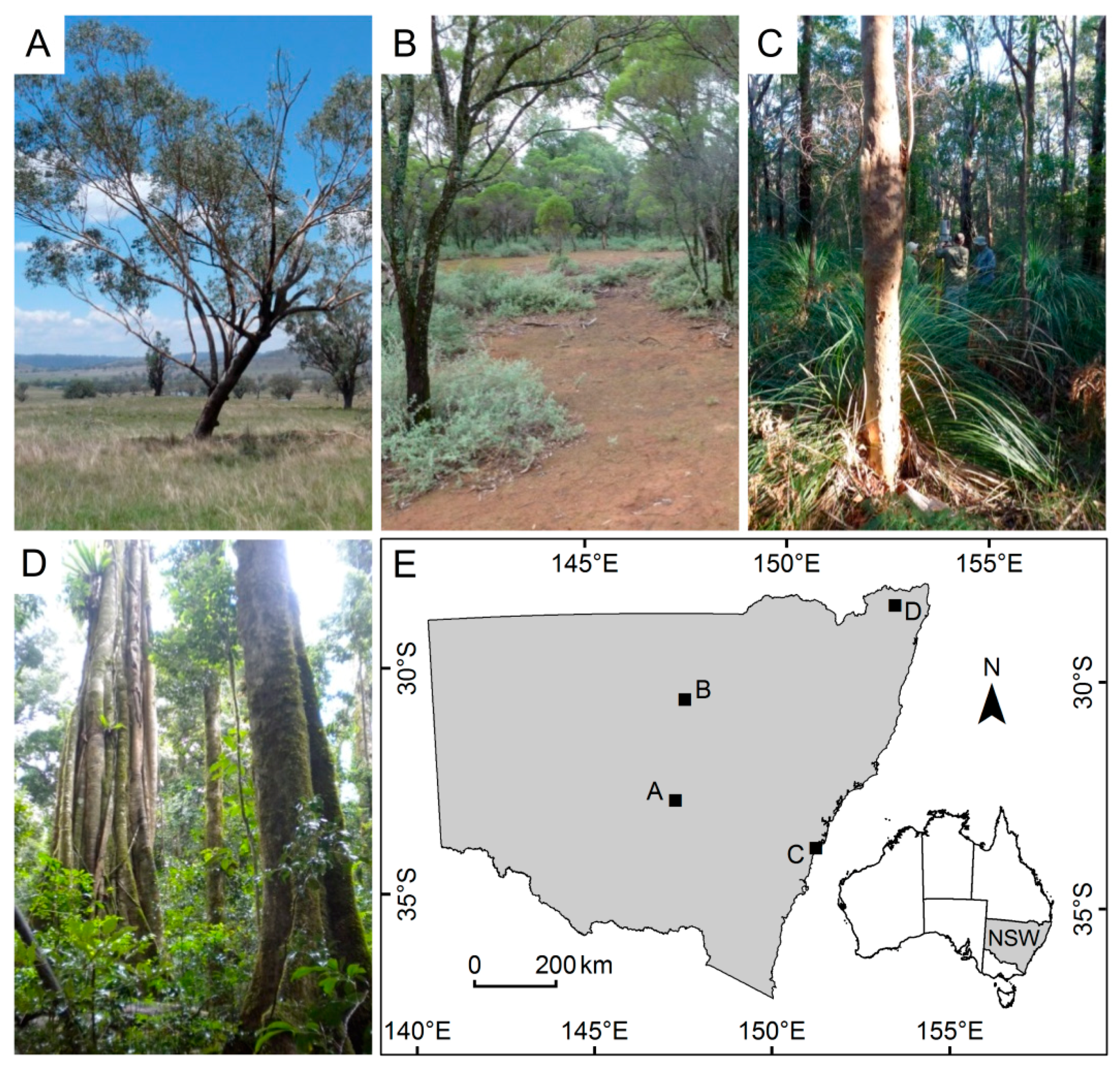
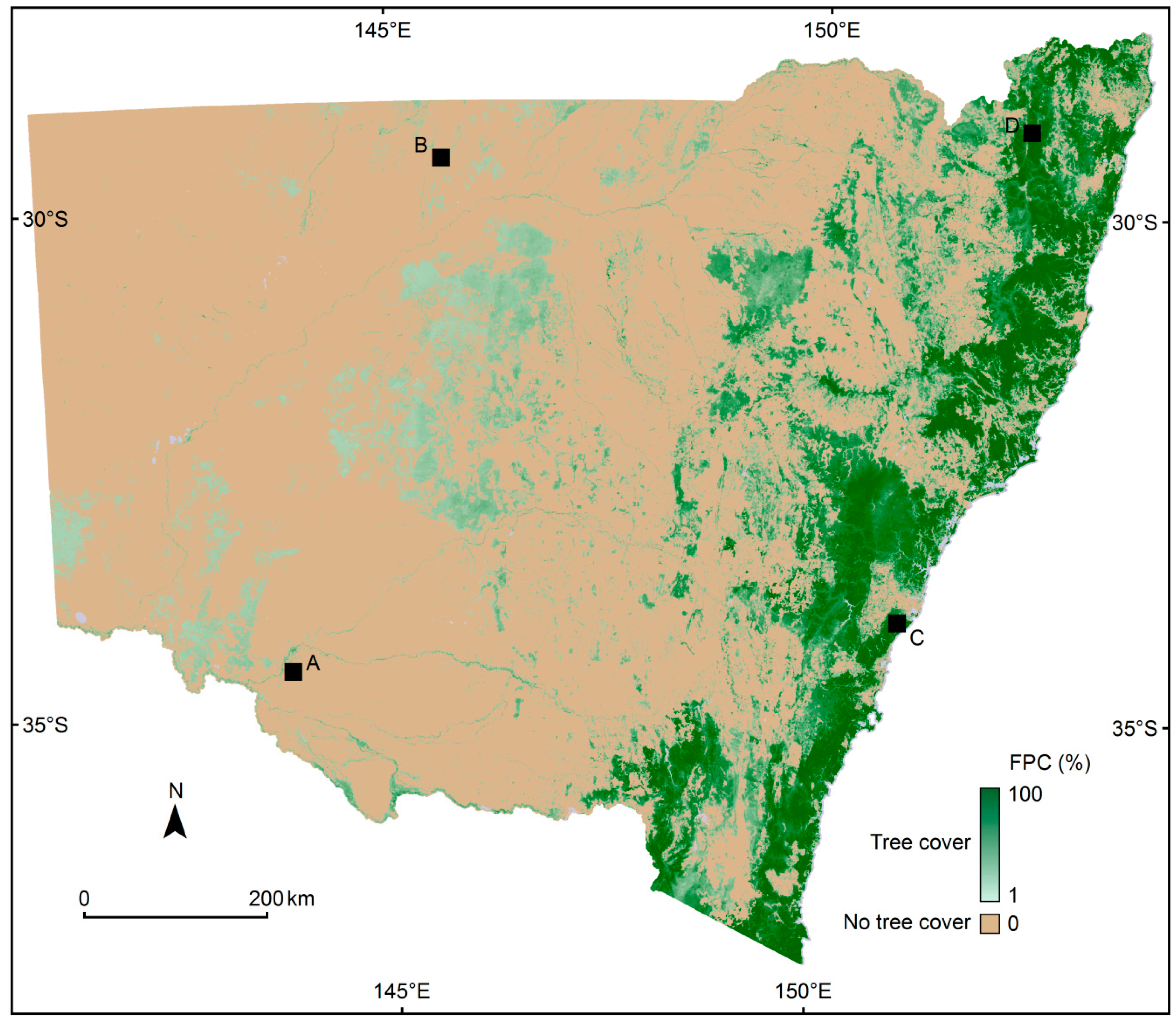
NSW is located on the central, eastern coast of Australia between 141°E and 154°E longitude and 28°S and 38°S latitude (
Figure 1). It covers a large area (809,444 km
2), across a wide range of climates (arid, temperate, subtropical, alpine) and has a variety of vegetation types such as shrublands, grasslands, woodlands and forests (
Figure 1). The climatic gradients strongly influence the main vegetation patterns: shrublands and grasslands in the arid west grade through to woodlands and then to forest in the humid east; species composition grades from warmer, wetter, subtropical forest in the northeast to cooler, temperate forest in the southeast [
30].
Tree clearing in NSW began following European settlement at Sydney in 1788, for both timber and to establish agricultural land, however it did not proliferate until the late 19th century with the expansion of the wheat and sheep industries [
7,
31]. Areas of fertile soil experienced the most clearing, with less productive ecosystems and areas of rugged terrain being left intact. Of the 99 vegetation classes mapped in 2004, 41 were estimated to have been cleared by over 30% [
30], leaving a highly fragmented landscape. In fragmented landscapes remnant patches of trees have been found to have a significant positive effect on ecosystems, even small fragments with low biomass [
32]. Ecosystem services provided by small remnant patches include: improvements to the abiotic environment via modifications to the local micro-climate [
32], water infiltration [
33], improved soil properties [
34] and the provision of resources to support local fauna [
35]. These studies show that although many remnant vegetation fragments are degraded, their presence provides vital ecosystem services and need to be conserved.
1.3. Tree Cover in the Australian Context
An accurate record of existing tree cover is particularly important in Australia, as it has lost nearly 40% of its forests [
7]. Prior to the work presented here, tree cover was mapped over NSW using Landsat data (25–30 m pixels), based on methods developed for the Queensland (QLD) Statewide Landcover and Trees Study (SLATS) [
25]. The SLATS method relied on a model between field measurements of foliage projective cover (FPC) and normalised Landsat data [
36]. FPC is the percentage of ground area covered by the vertical projection of foliage from tree crowns, and is commonly used in Australia [
37,
38]. Changes in FPC over time can be useful for detecting clearing, and distinguishing persistent tree foliage from temporary ground cover and understorey foliage.
Landsat based maps were a great improvement on previous products, however significant small patches of vegetation were still not mapped [
29,
39]. Farmer, Reinke and Jones [
29] compared tree cover derived from time series 25 m Landsat data [
28], 10 m SPOT4 data, and 0.15 m aerial photography, and found that tree cover mapped from sensors with pixel sizes greater than 10 m did not accurately detect small remnant patches of vegetation. Landscape fragmentation, product scale and minimum mappable unit were shown to influence the magnitude of error.
2. Materials and Methods
The method described here was adapted from that used previously across QLD and NSW with multi-temporal Landsat data, which allowed the separation of persistent tree cover from temporary vegetation cover [
25]. Instead of Landsat data, multi-temporal high spatial resolution imagery was purchased from the Satellite pour l’Observation de la Terre (SPOT5) High Resolution Geometric sensor. SPOT5 data was found to have a similar data quality to Landsat [
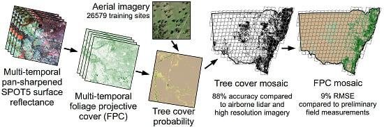
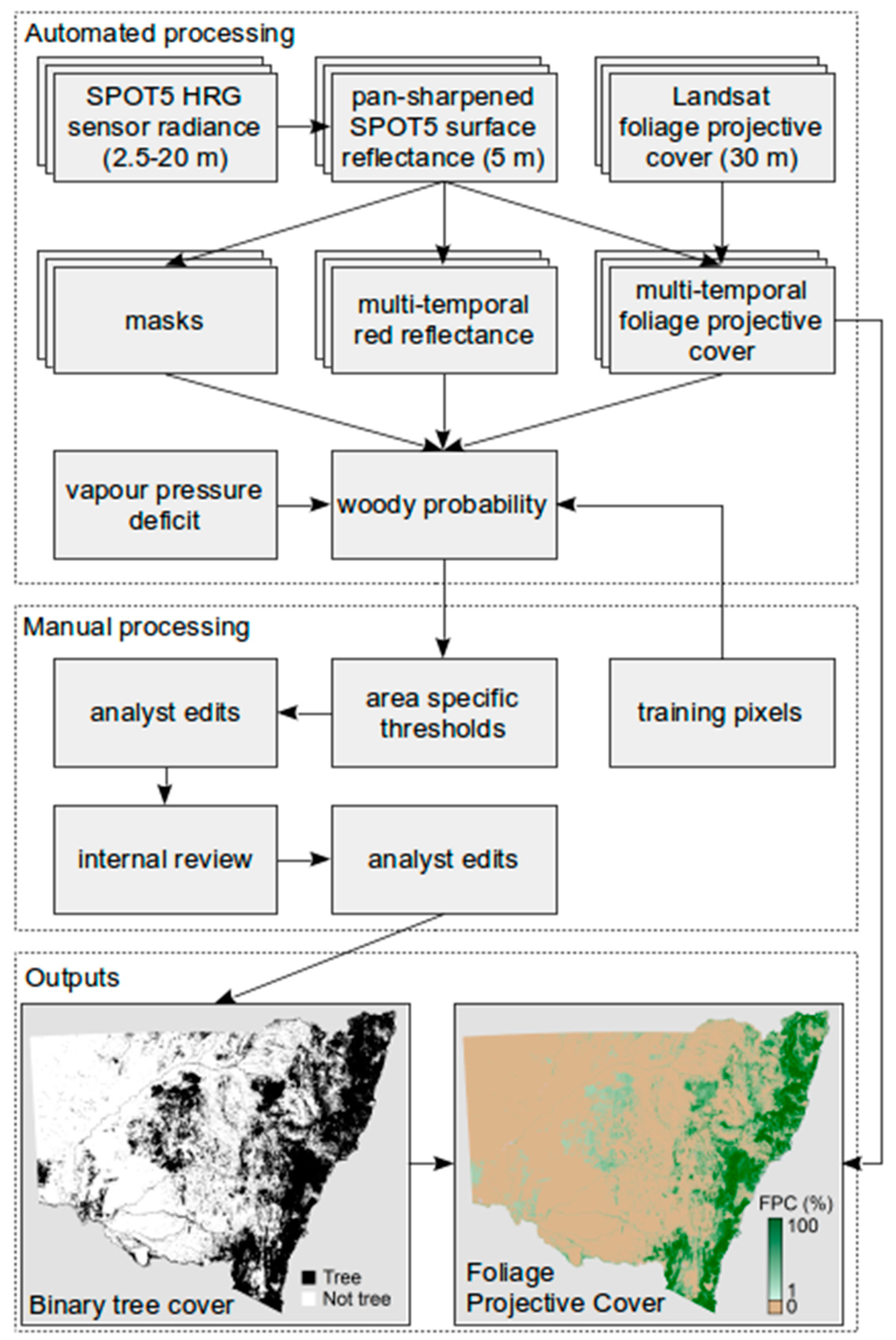
40], while providing a higher spatial resolution (2.5–20 m pixels). The main components of the method were: (1) pre-process and mask the SPOT5 data to pan-sharpened standardised surface reflectance; (2) model FPC from each SPOT5 image; (3) develop a multi-temporal model of tree cover probability; (4) derive a tree map from thresholding and editing of the probability model; (5) attribute the tree map with an estimate of FPC. These main steps are illustrated in
Figure 2 and described in more detail below.
2.1. Multi-Temporal SPOT5 Pan-Sharpened Surface Reflectance
A complete coverage of SPOT5 imagery was acquired for NSW from 2008, 2009, 2010 and 2011, for a total of 1256 images, with all parts of the state covered by pixels from the four time periods. Multi-temporal data were used as many trees and areas of herbaceous ground cover were found to be indistinguishable in single images, but could be separated in multi-temporal imagery due to the persistence of the tree foliage compared to the fluctuations in ground cover caused by a closer relationship to rainfall. The pointable, push-broom sensor produced multispectral imagery in three bands with 10 m pixels, one shortwave infrared band with 20 m pixels, and one panchromatic band with 2.5 m pixels. The spectral ranges are green (0.49–0.61 µm); red (0.61–0.68 µm); near infrared (NIR) (0.78–0.89 µm); shortwave infrared (SWIR) (1.58–1.75 µm), and panchromatic (0.49–0.69 µm). The images have a nominal swath width and path length of 60 km and were provided in units of calibrated, scaled, at-sensor radiance. Each image acquired needed to fulfil standard minimum specifications. They were nominally cloud free and the look angle was specified to be as close to nadir as possible and no more than 18 degrees off nadir. Images were preferentially obtained in summer months (November–March) when the grass cover was senescent, which provided good contrast to the green overstorey foliage [
36].
2.1.1. Ortho-Rectification
A geographic baseline image was created from SPOT5 panchromatic imagery captured in 2005. It was registered to a state-wide dataset of ground control points using a digital elevation model (DEM) and a satellite orbital model. In eastern NSW the DEM was based on topographic mapping data, and was supplied by Land and Property Information, the state government’s surveying agency. In western NSW the Shuttle Radar Topography Mission (SRTM) DEM was used. The baseline image was rectified to the ground control points with a root mean square error (RMSE) of 5 m. All other images were rectified to the baseline with an average RMSE of less than 3.75 m.
2.1.2. Surface Reflectance
The SPOT5 multispectral images were atmospherically corrected and adjusted for bi-directional reflectance and topography, representing surface reflectance with a nadir-view and a 45° incidence angle [
41]. Elevation data were obtained from the 1 s SRTM DEM [
42,
43,
44].
2.1.3. Pan-Sharpening
Each SPOT5 image was pan-sharpened to 5 m pixels, as although the panchromatic bands were supplied at 2.5 m resolution, they were acquired using 5 m resolution stereo instruments. The panchromatic bands were first degraded to 5 m and then used to sharpen the 10 m and 20 m bands to create 5 m resolution multi-spectral imagery. The Theil-Sen Estimator, a robust regression technique [
45], was used to fit linear relationships on a local, per-pixel basis using all the pixels in a 7 by 7 window based on high-resolution pixels (35 m by 35 m in this case), separately for each band. The method estimated the slope between two sets of points as the median of the slopes between all pairs of points. Using the local relationship, an estimate of the multi-spectral band was computed from the panchromatic band, at the higher resolution.
2.1.4. Mask Creation
Masks were created for each image at 10 m resolution. Although most images contained no or very little cloud, pixels contaminated by cloud and cloud-shadow were masked with a semi-automated object-based method, which included manual checking and editing [
46]. Surface water was identified and masked using a multi-dimensional water index method [
47]. The cast-shadow mask identified those pixels that lie in shadows cast from the surrounding topography, using a ray-casting technique [
48], which was simplified through assuming parallel rays of light. The extreme-angles mask identified those pixels with incidence (angle between surface normal and vector to sun) and exitance (angle between surface normal and vector to satellite) angles greater than 80°, which represent pixels with low signal to noise ratio due to little incidence or reflected light. The per-pixel surface normal, used in the calculation of these angles, was derived from the SRTM DEM.
2.2. Multi-Temporal Foliage Projected Cover
After pre-processing to pan-sharpened surface reflectance, each SPOT5 image was used to model FPC. Due to insufficient field data to calibrate a model, we related the surface-reflectance of the 5 m SPOT5 imagery to a Landsat derived overstorey FPC product [
25,
36]. The Landsat FPC product was trained using QLD field measurements of FPC, and applied with a multiple linear regression model to Landsat 5 TM and Landsat 7 ETM+ data [
36]. The QLD data and methods were made available through the Joint Remote Sensing Research Program (JRSRP) at the University of Queensland, which was established to improve the consistency of products across state borders. The QLD Landsat FPC model had a relatively low RMSE of 10.26% and 8.95% compared to field and lidar measurements, respectively [
36]. A preliminary unpublished validation of the model in NSW indicates that it has a similar accuracy.
To calibrate between sensors, 2485 data points were collected from a total of 60 SPOT5 images across NSW and QLD (
Figure 3A). Image locations were chosen to capture a large range of vegetation communities, land types, and variations in FPC. The multi-spectral SPOT5 images and Landsat FPC images were degraded to an area equivalent to 3 by 3 Landsat pixels (90 m by 90 m), before sample pixels were taken on a regular 1 km by 1 km grid. Only points that were on a slope of less than 5% (determined from the SRTM DEM) and within an area of homogenous tree cover (determined by the Landsat FPC), were used. These homogenous areas were defined where the coefficient of variation of the Landsat FPC in a 5 by 5 pixel window (150 m by 150 m) was less than 0.05. Degrading the images and choosing pixels on homogeneous sites reduced the influence of misregistration between the SPOT5 and Landsat FPC images on the model. Multiple linear regression was used to relate the SPOT5 reflectance to Landsat FPC and the adjusted
r2 of the model fit was 0.88. The model included terms for each SPOT5 band (
λi), and interactions between them:
where
F is FPC,
β are the coefficients, and the function
f used to remove skewness in the distribution [
36] was:
Although the model was developed using 90 m degraded imagery, it was applied on the 5 m resolution pan-sharpened SPOT5 surface reflectance data. In doing so, we assume that the multispectral surface reflectance and FPC models at 5 m and 90 m are linearly related.
2.3. Tree Cover Probability
A binomial logistic regression model was used to calculate the probability of a 5 m SPOT5 pixel containing tree cover. The explanatory variables tested were: a climatological variable; an indicator of brightness; an indicator of greenness; variation in brightness and greenness over time; and interactions between variables. The response variable was the presence or absence of tree cover. The model was trained using 25,930 image-interpreted points (
Figure 3B), which were selected using a stratified random sampling method. Stratification was based on thirteen major catchments exhibiting a variety of terrain and vegetation types, as well as the Landsat derived FPC. Each point was visually assessed against high resolution imagery (0.5–2.5 m pixels), and if it was located on a mixed pixel it was manually shifted to the nearest 3 by 3 pixel window (15 m by 15 m) that featured a complete cover of its stratified attribute. Any points that were obscured by cloud, cloud shadow or water in at least one image were removed.
A combination of brightness and greenness indicators were selected as explanatory variables as they had previously been shown to relate to soil, grass and tree cover features [
49]. Red reflectance was used as the indicator of brightness, and FPC was used as an indicator of greenness [
49]. The multi-temporal variables were calculated from the four observations for each pixel, and were used to separate persistent tree cover from fluctuating ground cover. Using robust regression to exclude outliers, linear models were fitted to the red reflectance and FPC time series. The fitted value at the midpoint of each time series was used in the modelling. The red reflectance was transformed by adding 0.001 and taking the natural logarithm to remove the skewness and improve the normality of the distribution [
36]. Overstorey vegetation tends to have low variation in red reflectance and FPC over time. As such, the variation in FPC and red reflectance, from the fitted line, expressed as the ratio of the fitted value at the midpoint was also used. The variation was calculated as the weighted mean residual of the points from the fitted line, where the weights were those returned from the robust regression.
The other parameter considered for the probability model was vapour pressure deficit (VPD), which was previously used to model FPC [
36]. VPD varies spatially and is related to vegetation foliage characteristics. In Australia, smaller needle-like foliage tends to be found in areas with high VPD, while larger broad-leaf foliage tends to be found in areas with low VPD. The overstorey vegetation in high VPD areas in the study area also tends to have lower FPC and brighter background reflectance than that in low VPD areas. To allow for these relationships we included interaction terms between the red reflectance and FPC, red reflectance and VPD, and FPC and VPD. The VPD data were obtained from a gridded dataset, interpolated from a network of weather stations [
50].
A variety of models was assessed, using the kappa statistic to determine how well they classified the training data, where a pixel was classified as tree cover when its probability was at least 50%. The best model, which achieved a kappa statistic of 0.81, used the following explanatory variables: FPC, red reflectance, VPD, and variation in FPC. The interactive explanatory variables did not increase the model accuracy. The final model was then applied to every pixel across NSW, creating a statewide probability image. As the robust regression required at least three observation in the time series, pixels with fewer than three observations due to missing data (e.g., from clouds) were assigned a null value (0.2% of the data).
2.4. Binary Tree Cover
The probability surface was used as the primary dataset in classifying tree cover pixels. The surface was split into 305 tiles across NSW where each tile was approximately 55 km by 57 km. These tiles approximate the size and location of the SPOT5 images, although due to the variable look angle of the sensor the images did not conform to the standard paths and rows of nadir-viewing sensors. A probability threshold was manually selected for each tile in order to classify tree cover pixels, as there was insufficient training data for optimum thresholds to be calculated using accuracy statistics. This was done interactively by visually discerning tree foliage in 2.5 m pan-sharpened SPOT5 near-natural imagery acquired during the 2011 summer. Due to variations in vegetation type and structure the effectiveness of any specific threshold varied spatially within each tile. To account for this, most tiles were iteratively refined by identifying sub-tile thresholds for specially digitised areas. This process removed most errors, although commission errors remained in some areas due to the presence of water or the inability of the time series to differentiate green herbaceous vegetation from tree cover. Omission errors from clouds also remained. Each tile was therefore further edited on-screen by visually comparing with the SPOT5 2.5 m imagery. Visible commission errors were manually erased and missing patches of contiguous forest were digitised.
The probability thresholds varied from 0–40 in the southwest to 60–98 in the northeast and along the coast. Southwest NSW had good separation of trees and non-trees in the probability image, and could have lower thresholds without causing large commission errors. Northeast NSW and coastal areas required higher thresholds to separate areas of cropping and wetland vegetation that had higher probability values due to persistent greenness. There was also severe flooding in this part of the state which affected vegetation growth greatly.
2.5. Foliage Projective Cover
Once the binary tree cover map was produced, each tree cover pixel was attributed with an estimate of FPC. This was calculated as the mean of the multi-temporal FPC values for each pixel, so as to smooth fluctuations in time and better represent persistent tree foliage. In nearly all cases, this was the mean of three or four values, as it was very rare to have a pixel masked more than once by cloud or cloud-shadow. The mean value was also calculated for persistently dark pixels present in areas of steep terrain, even though they may have been masked by the cast-shadow and/or extreme-angle masks. FPC in these areas is considered more uncertain, due to reduced signal-to-noise in the satellite measurements.
2.6. Validation
Rigorous validation is crucial in producing useful land cover products [
11,
51,
52,
53,
54]. However, the challenges, including a very large commitment of resources and time, have generally discouraged thorough validation in large scale, high resolution maps [
55]. Intensive field survey is not practical but airborne lidar data does offer opportunities for precise measurements of forest structure and cover [
10,
23,
36,
56].The use of relatively finer resolution satellite data as the basis of or as a component of large area land cover accuracy assessment has also been established [
57,
58,
59,
60,
61].
Our validation dataset consists of field surveys to assess the final FPC map, a classification of tree cover from a sub-sample of the extensive archive of lidar data available, and a large collection of binary tree cover samples based on the visual assessment of very high resolution reference imagery (
Figure 3C–E). As the number of field sites collected was small compared to the large area mapped, the lidar products and visually assessed imagery were needed to distinguish the many vegetation types present across NSW. Accuracy was assessed using these two independent datasets with different scales. The lidar products provided precise tree maps, where even short, thin and scattered trees were detected, and may include areas of trees that would not be mapped as such by visual interpretation. The high resolution imagery provided locations where trees were present or absent according to visual assessment, which is closer to representing what most mapping programs accomplish. Each of the datasets is described in more detail in the following sections.
2.6.1. Field Data
FPC was calculated from field measurements made at 76 sites across NSW, collected between 2009 and 2015 (
Figure 3). Each field site was located away from disturbances (>100 m from roads or buildings) and steep terrain, in a patch of homogeneous vegetation. They were measured during other projects, and although they were not randomly distributed across all vegetation communities, they cover a wide range of FPC values. At each site, the star transect method [
62] was used to record 300 vertical sighting tube observations of the overstorey (woody vegetation >2 m height), midstorey (woody vegetation ≤2 m height) and understorey (herbaceous plants <2 m height), from a circular area with a radius of 50 m. The location of each centre point was recorded using differential GPS to less than ±5 m. Overstorey FPC (
FPCo) was calculated according to the following equation from Armston, Denham, Danaher, Scarth and Moffiet [
36]:
where
Po,g was the proportion of overstorey green foliage observations and
Po,b was the proportion of overstorey branch observations (which are likely to occlude foliage from the observer). As the satellite derived FPC model would likely be sensitive to both overstorey and midstorey foliage, we also calculated the combined FPC of the overstorey and midstorey (
FPCo+m) as:
where
Pm,g was the proportion of midstorey green foliage observations.
2.6.2. Airborne Lidar Data
Many airborne discrete return lidar surveys have been acquired over NSW for government use, covering over 46,000 km
2 or 6% of the state (
Figure 3D). The surveys were not randomly distributed, as many lidar surveys were over rivers, wetlands and urban areas, where high resolution elevation models were required for flood modelling. A stratified sample of tiles was taken, where a lidar tile was randomly sampled from each of the 17 vegetation formation classes [
63] within each of the 11 NSW land management regions (LLS), excluding urban areas [
64]. The lidar subset contained 119 tiles of data, from 34 different surveys, covering around 347 km
2, equivalent to more than 13.8 million pixels at 5 m resolution. Most of the tiles were 2 km × 2 km, though some were 1 km × 1 km or rectangular strips ~1.4 km
2. The surveys were acquired throughout 2008–2013, by three lidar instruments. Flight heights ranged from 500–2250 m above ground, footprints ranged from 0.23–1.21 m, and mean pulse density ranged from 1.1–8.3 pulses/m
2. Maximum scan angle averaged 16°, with a maximum of 40° in one tile. More information on the lidar data is available in the
supplementary material.
Lidar data was sourced in the LAS file format with ground and building returns classified using industry standard methods. LAS files were converted to the Sorted Pulse Data (SPD) format [
65] and spatially sorted into bins aligning with the 5 m SPOT5 pixels. The height of each return above the ground was calculated using natural neighbour interpolation [
66]. Lidar plant projective cover (
PPC) was calculated as the proportion of first returns from the canopy, within a pixel area, using Equation (5) [
36]:
where
CV(
z) is the number of first returns higher than
z m above the ground,
CG is the number of first return counts from the ground. Following the method of Armston, Denham, Danaher, Scarth and Moffiet [
36],
z was set at 0.5 m, as trees greater than 2 m in height often have foliage lower than 2 m above the ground. Pixels where PPC > 0 and all returns were <2 m above the ground were considered understorey and not classified as tree cover. Maximum height of the vegetation was also derived as the 99th percentile of first return height. As each lidar tile created a spatially continuous map, the size of each contiguous region, and the distance of each pixel to the nearest pixel of the opposite class was also calculated.
As the lidar data were a stratified sample of the map area, the proportion of each stratum was used when calculating the error matrix statistics [
67]. The proportions were calculated from the final classified map, for the 34 strata (tree and non-tree pixels from each of the 17 vegetation formations). Standard errors of the accuracy measures were not calculated, as the sample was clustered, and not representative of the entire study area.
2.6.3. Visual Interpretation of High Resolution Imagery
High resolution imagery was available from a Leica ADS40 airborne digital camera (0.5 m) for most of the state, from the NSW government’s standard capture program. The ADS40 sensor is equipped with a SH52 sensor head with a field of view (swath angle) of 64° and multiple linear CCD’s of 12000 pixels each, enabling the capture of four spectral bands of information [
68]. The spectral ranges are blue (0.428–0.492 µm); green (0.533–0.587 µm); red (0.608–0.662 µm); near infrared (NIR) (0.833–0.887 µm). The sensor is flown in north-south direction and the resulting swaths are mosaicked together and colour balanced. As ADS40 imagery was not available in western NSW, alternative 2.5 m SPOT5 imagery from 2011 was used.
Validation points (6648 pixels) were selected across NSW using a stratified random approach, ensuring that tree and non-tree pixels (determined by the previous Landsat derived map) from the 13 major catchments were sampled (
Figure 3E). Each point was visually assessed against the high resolution imagery and classified as either tree or not-tree. The proportion of each stratum, determined from the Landsat map, was used when calculating the error matrix statistics, including the standard errors [
67].
3. Results
3.1. Foliage Projected Cover
3.1.1. Comparison to Landsat
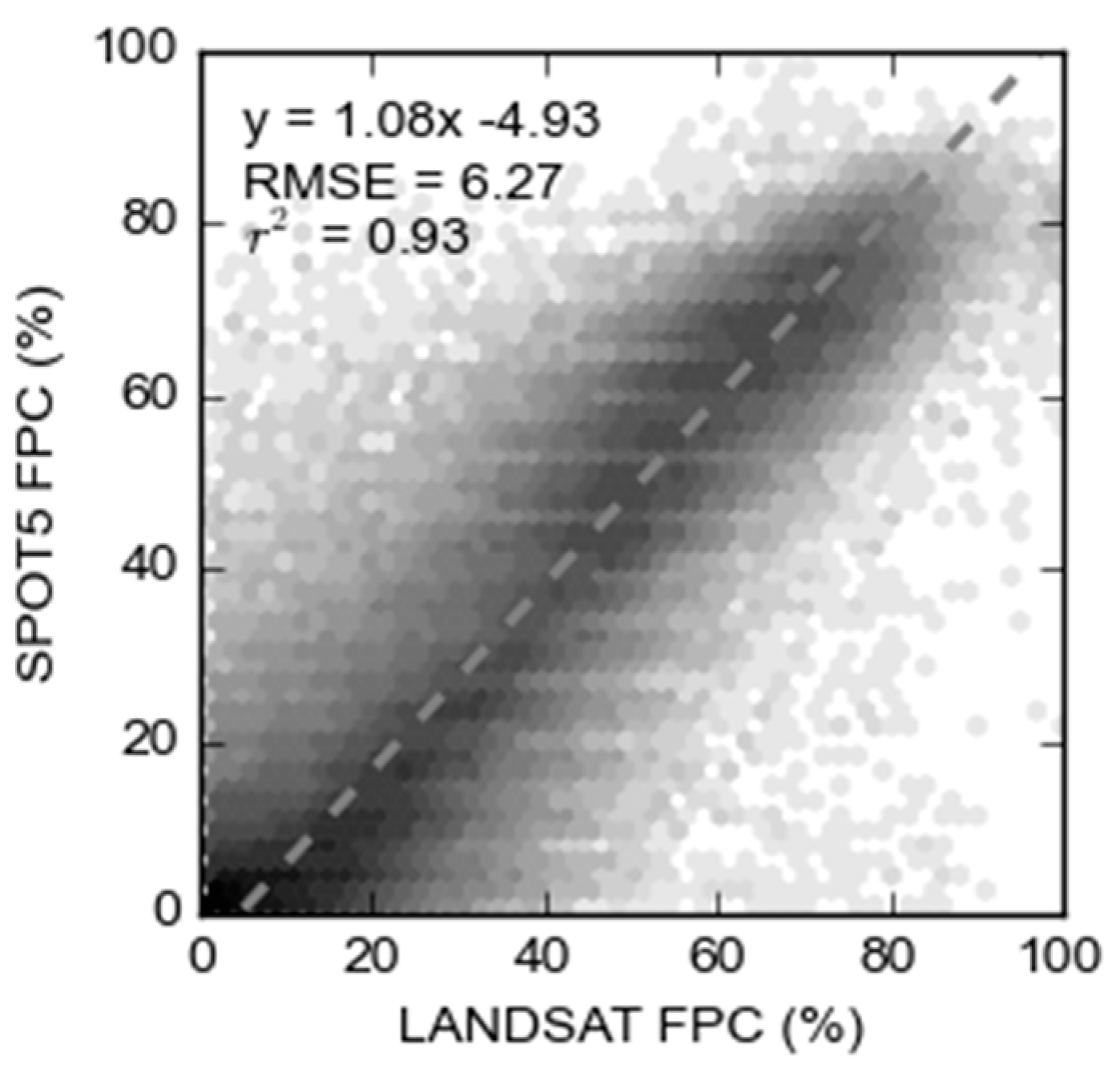
To determine how the new SPOT5 FPC map compared to the previous Landsat FPC map, both maps were degraded to 100 m pixels and a sample of areas selected using a regular 1 km grid across NSW. These areas were then sampled using a stratified random approach, to ensure that each vegetation formation class was evenly sampled, and only pixels classified as tree cover in both products were used. An orthogonal distance regression model was fit between the SPOT5 and Landsat FPC values, resulting in a very strong relationship (
r2 = 0.93, RMSE = 6.27) (
Figure 4). The results varied by vegetation formation, with SPOT5 overestimating FPC compared to Landsat in some vegetation types (Dry sclerophyll forests (Shrub/grass subformation), cleared, Semi-arid woodlands (Shrubby subformation), Dry sclerophyll forests (Shrubby subformation)), and underestimating in Arid shrublands (Acacia subformation). More information is available in the
supplementary material.
The results are useful as they indicate that the lower spectral resolution of the SPOT5 data was capable of modelling FPC, although the close relationship is not surprising given the SPOT5 FPC model was trained using the Landsat FPC data. However, the comparison does not assess the application of the model at 5 m resolution, which assumes a linear relationship between FPC at the different scales. This assumption is the focus of ongoing research.
3.1.2. Field Data
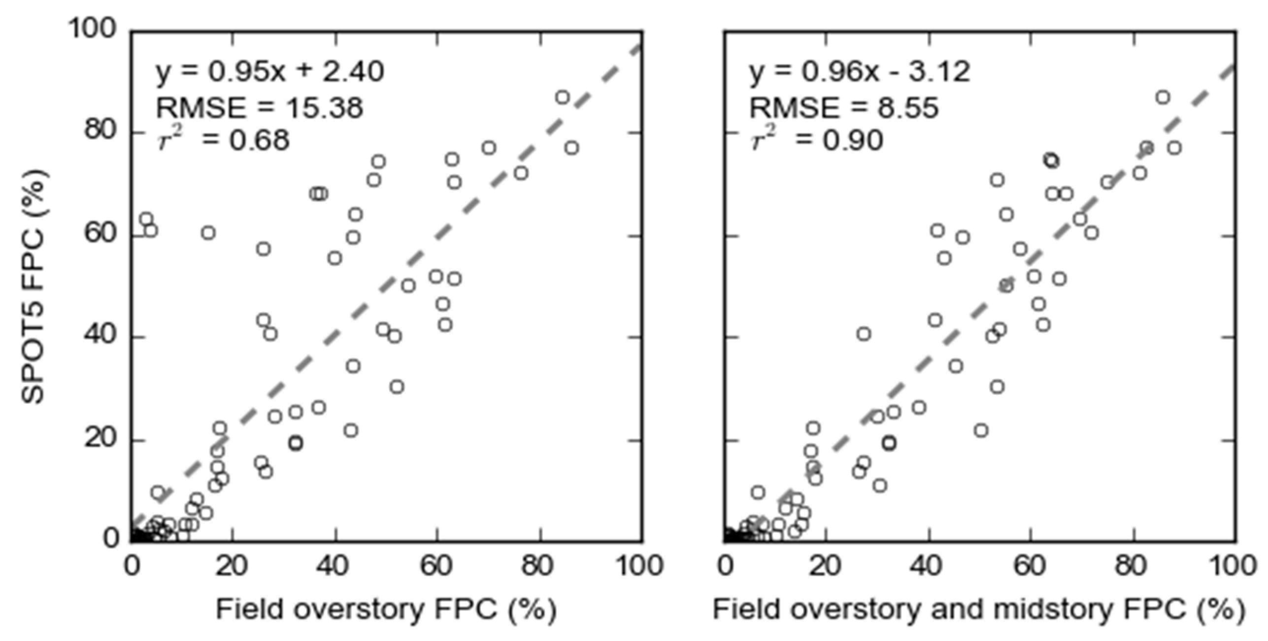
For each field site, the mean value of the SPOT5 FPC map was calculated from all pixels within a 55 m radius, and compared to the field measurements. Ordinary least squares regression revealed a weak positive linear relationship (
r2 = 0.66) between SPOT5 FPC values and the field measured overstorey FPC values, which improved to a very strong relationship (
r2 = 0.90) when the midstorey foliage was included in the field FPC values (
Figure 5). In general, the model slightly underestimated overstorey plus midstorey FPC, especially for values less than 40%. The validation of SPOT5 FPC using field data presented here should only be considered preliminary, and the statistics presented may not be representative of the statewide map due to the small sample size and the opportunistic sampling design.
3.2. Binary Tree Cover
3.2.1. Visual Assessment
The binary tree cover map achieved an overall accuracy (calculated as the total proportion of correctly classified pixels as a percentage of all pixels [
67]) of 88% (±0.51% standard error), when compared to the 6648 visually attributed reference pixels (
Table 1). Prior to editing and sub-tile thresholding the overall accuracy was 87%. Although the increase in accuracy due to manual editing appears small, it was not uniform across the state, as some areas required little or no editing while others required extensive revisions. For example, four of the catchment areas improved by 3%–4% in overall accuracy due to the manual editing. For the full accuracy assessment by catchment area see the
supplementary material. The manual editing was particularly effective in reducing the commission of false positive tree pixels. This was measured by the user’s accuracy for tree cover pixels (calculated as the proportion of correctly classified tree pixels as a percentage of the all classified tree pixels), which increased from 85% (±0.99%) to 90% (±0.73%) after editing (
Table 1).
The producer’s accuracy for tree cover pixels (also known as the true positive rate or TPR, calculated as the percentage of reference tree pixels that are correctly classified), was reduced after editing from 75% (±1.21%) to 73% (±1.21%). Although some of the manual editing targeted these omission errors, through sub-tile thresholding and digitising, it is clear that most were not corrected. This reflects the difficulty in mapping tree cover in fragmented landscapes.
The final binary tree cover classification performed well for most of the catchment areas, with eight of the 13 catchments having overall accuracies greater than 90%. The least accurate catchments were Western (82% ± 1.41%) and the Lower Murray-Darling (82% ± 1.69%).
3.2.2. Lidar
Validation of the final binary tree cover map against the lidar derived reference revealed very similar accuracies to the visual assessment (
Table 1), with an overall accuracy of 88% a TPR of 74%, a user’s accuracy of 89%, and a false positive rate (FPR) of 5%. FPR is the percentage of reference pixels incorrectly classified as tree cover. The lidar derived accuracies have more errors from false positive tree pixels and the omission of tree pixels, however the errors were not uniformly distributed across the state. The greatest omission errors were observed in arid shrublands, semi-arid woodlands and grasslands in the west, as well as cleared landscapes. The greatest commission errors were observed in, heathlands and wet sclerophyll forests, in the east. For the full accuracy assessment by vegetation formation see the
supplementary material.
Analysing the errors according to various lidar-derived vegetation categories revealed that omission errors decreased with increasing PPC and increasing height (
Table 2). This explains the omission errors observed in the west of the state, where the arid and semi-arid vegetation is generally shorter, has thinner canopies and greater spacing between trees. Commission errors increased as the maximum vegetation height approached 2 m (
Table 2), explaining the commission errors that were observed in areas of tall shrubs, such as heathlands, saline wetlands and dry sclerophyll forests with shrubby understory. Both omission and commission errors were more common for pixels on the edges of tree cover regions (
Table 2), which may have partly been caused by differences in georeferencing between the SPOT and lidar imagery, or the presence of tree shadows.
The size of continuous regions containing errors was also found to have an effect, where omission and commission were more likely in smaller regions (
Table 2). This indicates that the SPOT5 tree cover map has more errors in landscapes with fragmented, patchy tree cover, than in landscapes with large regions of similar vegetation.
Validation was also conducted on the tree cover with threshold prior to manual editing (
Table 1). This revealed that the manual editing increased the overall accuracy from 86% to 88%, and reduced the FPR for tree cover pixels from 8% to 5%. The editing decreased FPR across all vegetation formations, with some vegetation formations such as dry sclerophyll forests (grassy) showing large reductions (6%). These improvements in accuracy were most significant for pixels with low maximum height (0.0–0.5 m), that were greater than 20 m from a true tree cover pixel, and which were within large non-tree cover regions (>3 ha), where commission rates were more than halved (
Table 2).
4. Discussion
4.1. Map Accuracy
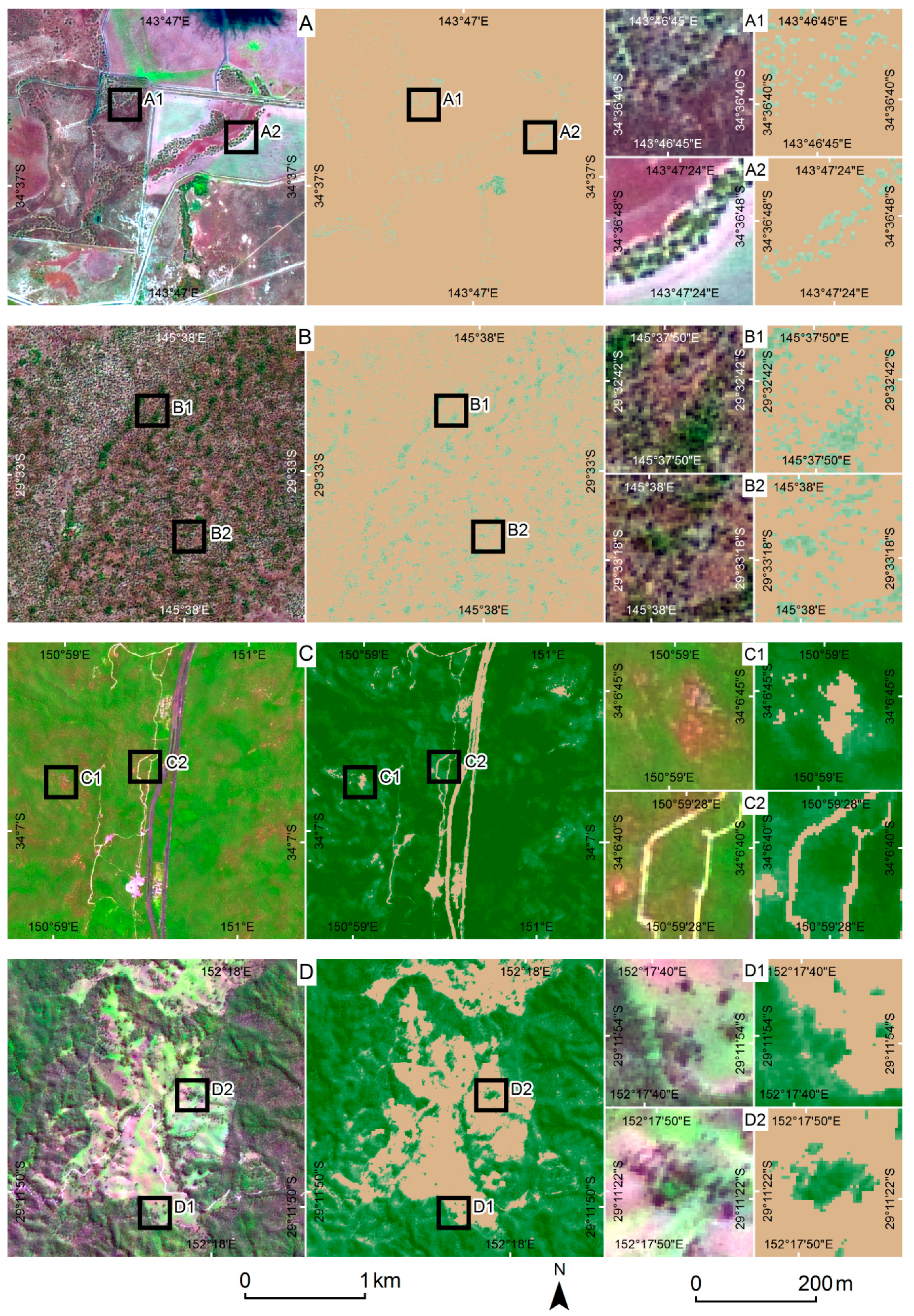
The high resolution binary tree cover map was found to have an accuracy of 88%, compared to lidar derived products and visually interpreted high resolution imagery. Visually comparing the map to the source SPOT5 imagery shows that it does a remarkably good job delineating the distribution of tree cover across the wide variety of landscapes present across NSW (
Figure 6 and
Figure 7).
Omission of trees was more common in arid shrublands and semi-arid woodlands, where the trees are shorter, have thinner canopies and are spaced further apart. Commission errors (false positive trees) were more common in areas containing tall shrubs, such as saline wetlands, heathlands, and dry sclerophyll forests (shrubby). Revealing this distribution of errors was only possible through the careful sampling of validation data, and the use of lidar derived products related to tree canopy density and height.
The probability scores over wetland areas were highly variable due to fluctuations in inundation and vegetation growth, making it difficult to apply appropriate sub-tile thresholds. The lower accuracies in arid shrubland vegetation types were caused by difficulties in detecting scattered trees with open canopies.
Over half the errors were identified as being close to the edges of tree pixels. These errors may be due partly to the difficulty in mapping thinner canopies around the edges of forest, but may have been caused by differences in georeferencing between the satellite and lidar data, or the influence of tree shadows. The size of regions containing errors was also found to have an effect, where omission and commission were more likely in smaller regions. This indicates that the SPOT5 tree cover map has more errors in landscapes with fragmented, patchy vegetation, and in clearings within large continuous regions of trees.
The SPOT5 FPC map showed an excellent agreement with the previous Landsat based map, when both maps were degraded to 100 m pixels. It also correlated very strongly with field measurements of FPC (overstorey and midstorey), made at 100 m diameter sites. These results confirm that the inclusion of multi-temporal data in the method reduced the influence of ground cover on the FPC map. Comparing to these field measurements, the SPOT5 tree cover map had a RMSE of around 9%, which is very similar to that observed in the QLD Landsat FPC model [
36]. Future work will focus on acquiring further field and lidar measurements of FPC to allow further analysis of these errors. Deriving FPC from airborne lidar by correcting for bias due to non-foliage canopy elements and varying survey-sensor parameters is the subject of ongoing research.
4.2. Statewide Distribution of Tree Cover
Overall, tree cover accounted for 27.11% of the area of NSW when mapped at the spatial resolution of 5 m. The spatial variability in tree cover reflects the ecology and disturbance history of the state. The most common vegetation mapped as tree cover was dry sclerophyll forest, with 8.67% of the State’s tree cover even though it is only 10.14% of the state. Also common are semi-arid woodlands, which contain 6.23% of the State’s tree cover, although they cover a greater area (52.85% of the state), revealing the scattered distribution of trees. The most common of the vegetation formations mapped by Keith and Simpson [
63] was cleared vegetation (37.03% of the state), which was found to have 9.96% tree cover, much of which occurs as scattered remnants and paddock trees. A full table of tree cover statistics is presented in the
supplementary material.
4.3. Future Research
The high accuracy of the tree cover map derived from SPOT5 data with 5 m pixels supports previous research that images with pixels less than or equal to 10 m are required to accurately map small patches of remnant vegetation [
29]. The use of multi-temporal data also contributed to the accurate mapping of tree cover and FPC, through distinguishing persistent overstorey tree cover from fluctuating understorey vegetation. Despite this, manual editing (selection of thresholds and local digitising) was still required to improve the utility of the final maps, mainly to reduce the commission of false positives due to persistent understorey vegetation. This editing was a time-consuming process, which future research should look at reducing. Two main options are apparent: increasing the temporal frequency of the imagery, or combining the multi-spectral data with information on vegetation structure derived from L-Band radar [
69,
70,
71].
Firstly, using more than four images across four years to model tree cover probability would capture more variation in understorey vegetation growth and senescence across the seasons and so improve the model accuracies. However, some vegetation types with no tree cover, such as evergreen pastures and wetlands, have grasses that rarely senesce and additional multi-spectral data may not improve the results. Furthermore, purchasing dense time-series of high resolution data for large areas would be prohibitively expensive. Free data from the Sentinel-2 satellite constellation will avoid this problem, and may provide the required spatial (10 m multispectral), spectral (13 bands), and temporal (5-day revisit cycle) characteristics to improve the current method.
Secondly, data from L-Band radar satellites, such as the Advanced Land Observing Satellite 2 (ALOS-2) Phased Array type L-band Synthetic Aperture Radar (PALSAR), are able to map differences in vegetation structure relating to the presence of tree trunks and branches [
69,
70,
71]. The combination of PALSAR and Landsat data has previously improved vegetation mapping in QLD [
69,
70,
71], and future research should investigate methods of combining with Sentinel-2 data.
5. Conclusions
The objective of this work was to develop a method to map the heterogeneous patterns of fragmented forest and open woodland across the Australian state of NSW. This was achieved through combining multi-temporal high spatial resolution data from the SPOT5 satellite, automated image processing methods developed for continental scale Landsat projects, and manual image processing methods developed for regional scale vegetation mapping. The result is a tree cover map with 5 m pixels, which will be used for natural resource management at a variety of scales, from state-wide reports to local planning.
Overall accuracy for the binary tree cover map was 88%, determined through comparison with high resolution imagery and airborne lidar data. Errors were not uniformly distributed, with omission of trees more common in the arid and semi-arid regions, and commission of false positive trees more common in areas of tall shrubs, such as heathlands and wetlands. Although the use of multi-temporal imagery allowed the classification to separate persistent tree cover from temporary fluctuations in ground cover, it proved too difficult in some areas. A preliminary assessment of the FPC tree cover map using a sample of 76 non-randomly selected field plots resulted in an RMSE of around 9%. Future work will examine methods of deriving FPC from airborne lidar data, to allow a larger validation sample. The validation of the map products, using field data, high resolution imagery and airborne lidar, was as thorough as possible, and provides extra information to map users who can determine practical limitations based on their knowledge of local vegetation. The lidar products were particularly informative, providing quantitative data on vegetation cover, height, and fragmentation.
As expected, the use of multi-temporal SPOT5 data over such a large area proved more computationally intensive than previous Landsat based projects. The fewer spectral bands that were available in the SPOT5 data proved capable of modelling FPC, and the smaller pixel size allowed much better depiction of the fragmented nature of the vegetation. Comparison of the SPOT5 and Landsat FPC maps showed excellent agreement, when both were degraded to 100 m pixels. Future tree cover maps based on 10 m multi-spectral Sentinel‑2 data may provide greater accuracy due to the increased spectral and temporal resolution, and will hopefully require less manual editing to reduce the commission of false positives due to persistent understorey vegetation.
The high degree to which Australian forests have been cleared and fragmented has created an imperative for the conservation of existing primary forest patches. It also highlights the importance of possible regeneration of areas between fragments to increase native habitat area, connectivity and ecosystem functions [
7]. The SPOT5 tree cover map presented here will facilitate better management and conservation across the fragmented vegetation of NSW.
Supplementary Materials
The following are available online at
www.mdpi.com/2072-4292/8/6/515/s1 in a supplementary document: Figure S1: Predicted SPOT5 FPC compared with the predicted Landsat FPC, for the 17 vegetation formation classes listed in Table S1, Table S1: Tree cover area for NSW grouped by vegetation formation, Table S2: Specifications of the lidar surveys sampled as part of the tree cover validation, Table S3: SPOT5 tree cover accuracy statistics using visually interpreted data as reference, grouped by catchment, Table S4: SPOT5 tree cover accuracy statistics using lidar products as reference, grouped by vegetation formation.
Acknowledgments
SPOT5 data were acquired from Airbus Defence and Space. Lidar data were supplied by NSW Land and Property Information and a number of commercial vendors funded from various sources. We owe a debt of gratitude to the staff, volunteers and students who edited the maps, including Ashlee Wakefield, Geoff Dale, Rhys Grogan, Megan Powell and Catherine Carney. The maps may be requested through the Office of Environment and Heritage’s spatial data catalogue (
http://mapdata.environment.nsw.gov.au). Search for
woody vegetation.
Author Contributions
M.D., A.R., T.G. and T.D. conceived and designed the project; T.G., T.D., N.F. and A.F. performed the image pre-processing and masking; N.F. developed the pan-sharpening method; T.G. led the development of the FPC and probability models; M.D. led the manual thresholding, editing, reference data collection and validation using high resolution imagery; A.F. assessed the maps using lidar and field data; A.F., M.D., T.G. and A.R. contributed to creating the figures; All authors contributed to writing the paper.
Conflicts of Interest
The authors declare no conflict of interest.
Abbreviations
The following abbreviations are used in this manuscript:
| ALOS-2 | Advanced Land Observing Satellite 2 |
| DEM | digital elevation model |
| FPC | foliage projective cover |
| FPR | false positive rate |
| JRSRP | Joint Remote Sensing Research Program |
| NIR | near infrared |
| NSW | New South Wales |
| PALSAR | Phased Array type L-band Synthetic Aperture Radar |
| PPC | plant projective cover |
| QLD | Queensland |
| RMSE | root mean square error |
| SLATS | Statewide Landcover and Trees Study |
| SPOT5 | Satellite pour l’Observation de la Terre 5 |
| SRTM | Shuttle Radar Topography Mission |
| SWIR | shortwave infrared |
| TPR | true positive rate |
| VPD | vapour pressure deficit |
References
- Haddad, N.M.; Brudvig, L.A.; Clobert, J.; Davies, K.F.; Gonzalez, A.; Holt, R.D.; Lovejoy, T.E.; Sexton, J.O.; Austin, M.P.; Collins, C.D.; et al. Habitat fragmentation and its lasting impact on Earth’s ecosystems. Sci. Adv. 2015, 1, e1500052. [Google Scholar] [CrossRef] [PubMed]
- Antos, M.; White, J. Birds of remnant vegetation on the Mornington Peninsula, Victoria, Australia: The role of interiors, edges and roadsides. Paci. Conserv. Biol. 2004, 9, 294–301. [Google Scholar] [CrossRef]
- Debuse, V.J.; King, J.; House, A.P.N. Effect of fragmentation, habitat loss and within-patch habitat characteristics on ant assemblages in semi-arid woodlands of Eastern Australia. Landsc. Ecol. 2007, 22, 731–745. [Google Scholar] [CrossRef]
- Ford, H.A.; Walters, J.R.; Cooper, C.B.; Debus, S.J.S.; Doerr, V.A.J. Extinction debt or habitat change?—Ongoing losses of woodland birds in North-Eastern New South Wales, Australia. Biol. Conserv. 2009, 142, 3182–3190. [Google Scholar] [CrossRef]
- Holland, G.J.; Bennett, A.F. Habitat fragmentation disrupts the demography of a widespread native mammal. Ecography 2010, 33, 841–853. [Google Scholar] [CrossRef]
- Ross, K.; Fox, B.; Fox, M. Changes to plant species richness in forest fragments: Fragment age, disturbance and fire history may be as important as area. J. Biogeogr. 2002, 29, 749–765. [Google Scholar] [CrossRef]
- Bradshaw, C.J.A. Little left to lose: Deforestation and forest degradation in Australia since European colonization. J. Plant Ecol. 2012, 5, 109–120. [Google Scholar] [CrossRef]
- Day, M.; Roff, A. Multi-temporal classification of woody vegetation using pan-sharpened SPOT-5 data. In Proceedings of the 16th Australasian Remote Sensing and Photogrammetry Conference (16 ARSPC), Melbourne, Australia, 20–28 August 2012.
- Hansen, M.C.; Potapov, P.V.; Moore, R.; Hancher, M.; Turubanova, S.A.; Tyukavina, A.; Thau, D.; Stehman, S.V.; Goetz, S.J.; Loveland, T.R.; et al. High-resolution global maps of 21st-century forest cover change. Science 2013, 342, 850–853. [Google Scholar] [CrossRef] [PubMed]
- Sexton, J.O.; Song, X.-P.; Feng, M.; Noojipady, P.; Anand, A.; Huang, C.; Kim, D.-H.; Collins, K.M.; Channan, S.; DiMiceli, C.; et al. Global, 30-m resolution continuous fields of tree cover: Landsat-based rescaling of MODIS vegetation continuous fields with lidar-based estimates of error. Int. J. Digit. Earth 2013, 6, 427–448. [Google Scholar] [CrossRef]
- Pengra, B.; Long, J.; Dahal, D.; Stehman, S.V.; Loveland, T.R. A global reference database from very high resolution commercial satellite data and methodology for application to Landsat derived 30 m continuous field tree cover data. Remote Sens. Environ. 2015, 165, 234–248. [Google Scholar] [CrossRef]
- Arroyo, L.A.; Johansen, K.; Armston, J.; Phinn, S. Integration of lidar and quickbird imagery for mapping riparian biophysical parameters and land cover types in Australian tropical savannas. For. Ecol. Manag. 2010, 259, 598–606. [Google Scholar] [CrossRef]
- Brink, A.B.; Eva, H.D. Monitoring 25 years of land cover change dynamics in Africa: A sample based remote sensing approach. Appl. Geogr. 2009, 29, 501–512. [Google Scholar] [CrossRef]
- Cacetta, P.; Furby, S.; Wallace, J.; Wu, X.; Richards, G.; Waterworth, R. Long-term monitoring of Australian land cover change using landsat data: Development, implementation, and operation. In Global Forest Monitoring from Earth Observation; Frederic, A., Hansen, M., Eds.; CRC Press: Boca Raton, FL, USA, 2012; pp. 229–244. [Google Scholar]
- Homer, C.G.; Dewitz, J.A.; Yang, L.; Jin, S.; Danielson, P.; Xian, G.; Coulston, J.; Herold, N.D.; Wickham, J.D.; Megown, K. Completion of the 2011 national land cover database for the conterminous united states-representing a decade of land cover change information. Photogramm. Eng. Remote Sens. 2015, 81, 345–354. [Google Scholar]
- Yemshanov, D.; McKenney, D.W.; Pedlar, J.H. Mapping forest composition from the Canadian national forest inventory and land cover classification maps. Environ. Monit. Assess. 2012, 184, 4655–4669. [Google Scholar] [CrossRef] [PubMed]
- Asner, G.P.; Knapp, D.E.; Broadbent, E.N.; Oliveira, P.J.C.; Keller, M.; Silva, J.N. Selective logging in the Brazilian Amazon. Science 2005, 310, 480–482. [Google Scholar] [CrossRef] [PubMed]
- Hansen, M.C.; Stehman, S.V.; Potapov, P.V. Quantification of global gross forest cover loss. Proc. Natl. Acad. Sci. USA 2010, 107, 8650–8655. [Google Scholar] [CrossRef] [PubMed]
- Lehmann, E.A.; Wallace, J.F.; Caccetta, P.A.; Furby, S.L.; Zdunic, K. Forest cover trends from time series Landsat data for the Australian continent. Int. J. Appl. Earth Obs. Geoinf. 2013, 21, 453–462. [Google Scholar] [CrossRef]
- Townshend, J.R.; Masek, J.G.; Huang, C.; Vermote, E.F.; Gao, F.; Channan, S.; Sexton, J.O.; Feng, M.; Narasimhan, R.; Kim, D.; et al. Global characterization and monitoring of forest cover using Landsat data: Opportunities and challenges. Int. J. Dig. Earth 2012, 5, 373–397. [Google Scholar] [CrossRef]
- Asner, G.P.; Knapp, D.E.; Balaji, A. Automated mapping of tropical deforestation and forest degradation: CLASlite. J. Appl. Remote Sens. 2009, 3, 033543. [Google Scholar] [CrossRef]
- Huang, C.; Yang, L.; Wylie, B.; Homer, C. A strategy for estimating tree canopy density using Landsat 7 ETM+ and high resolution images over large areas. In Proceedings of the Third International Conference on Geospatial Information in Agriculture And Forestry, Denver, CO, USA, 5–7 November 2001.
- Alexander, C.; Bøcher, P.K.; Arge, L.; Svenning, J.-C. Regional-scale mapping of tree cover, height and main phenological tree types using airborne laser scanning data. Remote Sens. Environ. 2014, 147, 156–172. [Google Scholar] [CrossRef]
- Carreiras, J.M.B.; Pereira, J.M.C.; Pereira, J.S. Estimation of tree canopy cover in evergreen oak woodlands using remote sensing. For. Ecol. Manag. 2006, 223, 45–53. [Google Scholar] [CrossRef]
- Danaher, T.; Scath, P.; Armston, J.; Collett, L.; Kitchen, J.; Gillingham, S. Remote sensing of tree-grass systems: The eastern Australian woodlands. In Ecosystem Function in Savannas: Measurement and Modeling at Landscape to Global Scales; Hill, M.J., Hanan, N.P., Eds.; CRC Press: Boca Raton, FL, USA, 2010; pp. 175–194. [Google Scholar]
- Lucas, R.M.; Clewley, D.; Accad, A.; Butler, D.; Armston, J.; Bowen, M.; Bunting, P.; Carreiras, J.; Dwyer, J.; Eyre, T.; et al. Mapping forest growth and degradation stage in the Brigalow Belt Bioregion of Australia through integration of ALOS PALSAR and Landsat-derived foliage projective cover data. Remote Sens. Environ. 2014, 155, 42–57. [Google Scholar] [CrossRef] [Green Version]
- Tansey, K.; Chambers, I.; Anstee, A.; Denniss, A.; Lamb, A. Object-oriented classification of very high resolution airborne imagery for the extraction of hedgerows and field margin cover in agricultural areas. Appl. Geogr. 2009, 29, 145–157. [Google Scholar] [CrossRef]
- Furby, S.L.; Caccetta, P.A.; Wallace, J.F.; Lehmann, E.A.; Zdunic, K. Recent development in vegetation monitoring products from Australia’s national carbon accounting system. In Proceedings of the International Geoscience and Remote Sensing Symposium, Cape Town, South Africa, 12–17 July 2009; Volume 4, pp. 276–279.
- Farmer, E.; Reinke, K.J.; Jones, S.D. A current perspective on Australian woody vegetation maps and implications for small remnant patches. J. Spat. Sci. 2011, 56, 223–240. [Google Scholar] [CrossRef]
- Keith, D.A. Ocean Shores to Desert Dunes: The Native Vegetation of New South Wales and the Act; Department of Environment and Conservation: Hurstville, Australia, 2004.
- Norton, T. Conserving biological diversity in Australia’s temperate eucalypt forests. For. Ecol. Manag. 1996, 85, 21–33. [Google Scholar] [CrossRef]
- Manning, A.D.; Fischer, J.; Lindenmayer, D.B. Scattered trees are keystone structures—Implications for conservation. Biol. Conserv. 2006, 132, 311–321. [Google Scholar] [CrossRef]
- Eldridge, D.; Freudenberger, D. Ecosystem wicks: Woodland trees enhance water infiltration in a fragmented agricultural landscape in Eastern Australia. Austral Ecol. 2005, 30, 336–347. [Google Scholar] [CrossRef]
- Wilson, B. Influence of scattered paddock trees on surface soil properties: A study of the northern tablelands of NSW. Ecol. Manag. Restor. 2002, 3, 211–219. [Google Scholar] [CrossRef]
- Fischer, J.; Lindenmayer, D.B. Small patches can be valuable for biodiversity conservation: Two case studies on birds in southeastern Australia. Biol. Conserv. 2002, 106, 129–136. [Google Scholar] [CrossRef]
- Armston, J.D.; Denham, R.J.; Danaher, T.J.; Scarth, P.F.; Moffiet, T.N. Prediction and validation of foliage projective cover from Landsat-5 TM and Landsat-7 ETM+ imagery. J. Appl. Remote Sens. 2009, 3, 033540. [Google Scholar] [CrossRef]
- Walker, J.; Hopkins, M.S. Australian soil and land survey: Field handbook. In Australian Soil and Land Survey: Field Handbook, 2nd ed.; McDonald, R.C., Isbell, R.F., Speight, J.G., Walker, J., Hopkins, M.S., Eds.; CSIRO: Canberra, Australia, 1990; p. 190. [Google Scholar]
- Specht, R.L. Foliage projective covers of overstory and understory strata of mature vegetation in Australia. Austral Ecol. 1983, 8, 433–439. [Google Scholar] [CrossRef]
- Carruthers, S.; Bickerton, H.; Carpenter, G.; Brook, A.; Hodder, M. A Landscape Approach to Determine the Ecological Value of Paddock Trees: Summary Report Years 1 and 2; Department of Water Land and Biodiversity Conservation: Adeliade, Australia, 2004.
- Gill, T.; Clark, A.; Scarth, P.; Danaher, T.; Gillingham, S.; Armston, J.; Phinn, S. Alternatives to Landsat-5 Thematic Mapper for operational monitoring of vegetation cover: Considerations for natural resource management agencies. Can. J. Remote Sens. 2010, 36, 682–698. [Google Scholar] [CrossRef]
- Flood, N.; Danaher, T.; Gill, T.; Gillingham, S. An operational scheme for deriving standardised surface reflectance from Landsat TM/ETM+ and SPOT HRG imagery for eastern Australia. Remote Sens. 2013, 5, 83–109. [Google Scholar] [CrossRef]
- Farr, T.G.; Rosen, P.A.; Caro, E.; Crippen, R.; Duren, R.; Hensley, S.; Kobrick, M.; Paller, M.; Rodriguez, E.; Roth, L.; et al. The Shuttle Radar Topography mission. Rev. Geophys. 2007, 45, RG2004. [Google Scholar] [CrossRef]
- Gallant, J.; Read, A. Enhancing the SRTM data for Australia. In Proceedings of the Geomorphometry, Zurich, Switzerland, 31 August–2 September 2009.
- Gallant, J. 1 Second SRTM Level 2 Derived Digital Surface Model (DSM) v1.0; Geoscience Australia: Canberra, Australia, 2010.
- Sen, P.K. Estimates of the regression coefficient based on Kendall’s tau. J. Am. Stat. Assoc. 1968, 63, 1379–1389. [Google Scholar] [CrossRef]
- Fisher, A. Cloud and cloud-shadow detection in SPOT5 HRG imagery with automated morphological feature extraction. Remote Sens. 2014, 6, 776–800. [Google Scholar] [CrossRef]
- Fisher, A.; Danaher, T. A water index for SPOT5 HRG satellite imagery, New South Wales, Australia, determined by linear discriminant analysis. Remote Sens. 2013, 5, 5907–5925. [Google Scholar] [CrossRef]
- Robertson, K. Spatial transformation for rapid scan-line surface shadowing. IEEE Comput. Graph. Appl. 1989, 9, 30–38. [Google Scholar] [CrossRef]
- Moffiet, T.; Armston, J.D.; Mengersen, K. Motivation, development and validation of a new spectral greenness index: A spectral dimension related to foliage projective cover. ISPRS J. Photogramm. Remote Sens. 2010, 65, 26–41. [Google Scholar] [CrossRef]
- Jeffrey, S.J.; Carter, J.O.; Moodie, K.B.; Beswick, A.R. Using spatial interpolation to construct a comprehensive archive of Australian climate data. Environ. Model. Softw. 2001, 16, 309–330. [Google Scholar] [CrossRef]
- Boggs, G.S. Assessment of SPOT 5 and quickbird remotely sensed imagery for mapping tree cover in savannas. Int. J. Appl. Earth Obs. Geoinf. 2010, 12, 217–224. [Google Scholar] [CrossRef]
- Olofsson, P.; Stehman, S.V.; Woodcock, C.E.; Sulla-Menashe, D.; Sibley, A.M.; Newell, J.D.; Friedl, M.A.; Herold, M. A global land-cover validation data set, Part I: Fundamental design principles. Int. J. Remote Sens. 2012, 33, 5768–5788. [Google Scholar] [CrossRef]
- White, M.A.; Shaw, J.D.; Ramsey, R.D. Accuracy assessment of the vegetation continuous field tree cover product using 3954 ground plots in the south-western USA. Int. J. Remote Sens. 2005, 26, 2699–2704. [Google Scholar] [CrossRef]
- Wickham, J.D.; Stehman, S.V.; Fry, J.A.; Smith, J.H.; Homer, C.G. Thematic accuracy of the NLCD 2001 land cover for the conterminous United States. Remote Sens. Environ. 2010, 114, 1286–1296. [Google Scholar] [CrossRef]
- Herold, M.; Latham, J.S.; Di Gregorio, A.; Schmullius, C.C. Evolving standards in land cover characterization. J. Land Use Sci. 2006, 1, 157–168. [Google Scholar] [CrossRef]
- Wulder, M.A.; White, J.C.; Nelson, R.F.; Næsset, E.; Ørka, H.O.; Coops, N.C.; Hilker, T.; Bater, C.W.; Gobakken, T. Lidar sampling for large-area forest characterization: A review. Remote Sens. Environ. 2012, 121, 196–209. [Google Scholar] [CrossRef]
- Bontemps, S.; Langner, A.; Defourny, P. Monitoring forest changes in borneo on a yearly basis by an object-based change detection algorithm using SPOT-VEGETATION time series. Int. J. Remote Sens. 2012, 33, 4673–4699. [Google Scholar] [CrossRef]
- De Fries, R.S.; Hansen, M.; Townshend, J.R.G.; Sohlberg, R. Global land cover classifications at 8 km spatial resolution: The use of training data derived from Landsat imagery in decision tree classifiers. Int. J. Remote Sens. 1998, 19, 3141–3168. [Google Scholar] [CrossRef]
- Mayaux, P.; Pekel, J.F.; Desclee, B.; Donnay, F.; Lupi, A.; Achard, F.; Clerici, M.; Bodart, C.; Brink, A.; Nasi, R.; et al. State and evolution of the African rainforests between 1990 and 2010. Philos. Trans. R. Soc. Lond. Ser. B Biol. Sci. 2013, 368, 20120300. [Google Scholar] [CrossRef] [PubMed] [Green Version]
- Montesano, P.M.; Nelson, R.; Sun, G.; Margolis, H.; Kerber, A.; Ranson, K.J. Modis tree cover validation for the circumpolar taiga–tundra transition zone. Remote Sens. Environ. 2009, 113, 2130–2141. [Google Scholar] [CrossRef]
- Raši, R.; Bodart, C.; Stibig, H.-J.; Eva, H.; Beuchle, R.; Carboni, S.; Simonetti, D.; Achard, F. An automated approach for segmenting and classifying a large sample of multi-date Landsat imagery for pan-tropical forest monitoring. Remote Sens. Environ. 2011, 115, 3659–3669. [Google Scholar] [CrossRef]
- Muir, J.; Schmidt, M.; Tindall, D.; Trvithick, R.; Scarth, P.; Stewart, J. Field Measurement of Fractional Ground Cover: A Technical Handbook Supporting Ground Cover Monitoring for Australia; Queensland Department of Environment and Resource Management for the Australian Bureau of Agricultural and Resource Economics and Sciences: Canberra, Australia, 2011.
- Keith, D.A.; Simpson, C.C. Vegetation Formations of Nsw, Version 3.01 (vis-id 3848); Office of Environment and Heritage: Hurstville, Australia, 2010.
- Pink, B. Australian Statistical Geography Standard (Asgs): Volume 4—Significant Urban Areas, Urban Centres and Localities; Australian Bureau of Statistics: Canberra, Australia, 2012.
- Bunting, P.; Armston, J.; Lucas, R.M.; Clewley, D. Sorted pulse data (SPD) library. Part I: A generic file format for lidar data from pulsed laser systems in terrestrial environments. Comput. Geosci. 2013, 56, 197–206. [Google Scholar] [CrossRef]
- Bunting, P.; Armston, J.; Clewley, D.; Lucas, R.M. Sorted pulse data (SPD) library. Part II: A processing framework for lidar data from pulsed laser systems in terrestrial environments. Comput. Geosci. 2013, 56, 207–215. [Google Scholar] [CrossRef]
- Stehman, S.V. Estimating area and map accuracy for stratified random sampling when the strata are different from the map classes. Int. J. Remote Sens. 2014, 35, 4923–4939. [Google Scholar] [CrossRef]
- Sandau, R.; Braunecker, B.; Driescher, H.; Eckardt, A.; Hilbert, S.; Hutton, J.; Kirchhofer, W.; Lithopoulos, E.; Reulke, R.; Wicki, S. Design principles of the LH systems ADS40 airborne digital sensor. Int. Arch. Photogramm. Remote Sens. 2000, XXXIII Part B1, 258–265. [Google Scholar]
- Clewley, D.; Lucas, R.; Accad, A.; Armston, J.; Bowen, M.; Dwyer, J.; Pollock, S.; Bunting, P.; McAlpine, C.; Eyre, T.; et al. An approach to mapping forest growth stages in Queensland, Australia through integration of ALOS PALSAR and Landsat sensor data. Remote Sens. 2012, 4, 2236–2255. [Google Scholar] [CrossRef] [Green Version]
- Lucas, R.; Cronin, N.; Moghaddam, M.; Lee, A.; Armston, J.; Bunting, P.; Witte, C. Integration of radar and Landsat-derived foliage projected cover for woody regrowth mapping, Queensland, Australia. Remote Sens. Environ. 2006, 100, 388–406. [Google Scholar] [CrossRef]
- Lucas, R.; Armston, J.; Carreiras, J.; Nugroho, N.; Clewley, D.; de Grandi, F. Advances in the integration of ALOS PALSAR and Landsat sensor data for forest characterisation, mapping and monitoring. In Proceedings of the 2010 IEEE International Geoscience and Remote Sensing Symposium, Honolulu, HI, USA, 25–30 July 2010; pp. 1851–1854.
© 2016 by the authors; licensee MDPI, Basel, Switzerland. This article is an open access article distributed under the terms and conditions of the Creative Commons Attribution (CC-BY) license (http://creativecommons.org/licenses/by/4.0/).


