Generation of Land Cover Maps through the Fusion of Aerial Images and Airborne LiDAR Data in Urban Areas

Abstract

Satellite images and aerial images with high spatial resolution have improved visual interpretation capabilities. The use of high-resolution images has rapidly grown and has been extended to various fields, such as military surveillance, disaster monitoring, and cartography. However, many problems were encountered in which one object has a variety of spectral properties and different objects have similar spectral characteristics in terms of land cover. The problems are quite noticeable, especially for building objects in urban environments. In the land cover classification process, these issues directly decrease the classification accuracy by causing misclassification of single objects as well as between objects. This study proposes a method of increasing the accuracy of land cover classification by addressing the problem of misclassifying building objects through the output-level fusion of aerial images and airborne Light Detection and Ranging (LiDAR) data. The new method consists of the following three steps: (1) generation of the segmented image via a process that performs adaptive dynamic range linear stretching and modified seeded region growth algorithms; (2) extraction of building information from airborne LiDAR data using a planar filter and binary supervised classification; and (3) generation of a land cover map using the output-level fusion of two results and object-based classification. The new method was tested at four experimental sites with the Min-Max method and the SSI-nDSM method followed by a visual assessment and a quantitative accuracy assessment through comparison with reference data. In the accuracy assessment, the new method exhibits various advantages, including reduced noise and more precise classification results. Additionally, the new method improved the overall accuracy by more than 5% over the comparative evaluation methods. The high and low patterns between the overall and building accuracies were similar. Thus, the new method is judged to have successfully solved the inaccuracy problem of classification that is often produced by high-resolution images of urban environments through an output-level fusion technique.

1. Introduction

Recently, it has become possible to obtain optical images, Synthetic Aperture Radar images, aerial images, and airborne Light Detection and Ranging (LiDAR) data with different resolutions and characteristics using a variety of platforms. Because each data type includes different amounts of information and characteristics, a greater synergistic effect might be produced by their fusion [1]. For example, a better-quality land cover map can be produced by the combined use of an optical image and other data with different characteristics. Airborne LiDAR data in various spatial datasets have the advantage of being used to efficiently address the problems arising in the generation process of land cover classification using only high-resolution images in an urban area. Airborne LiDAR is composed of a laser scanner, the Global Navigation Satellite System, and the Inertial Navigation System and acquires height information of the terrain and objects on the surface at a high speed. This tool is suitable for the detection of buildings using height information and is used in a wide variety of fields, such as modeling, constructing 3D city models, urban planning, vegetation monitoring, and disaster management [2]. Thus, many studies on the generation of land cover maps through the data fusion of optical images and airborne LiDAR data using height information have been performed.

Data fusion is a process that takes data and information from multiple sources to produce refined and improved information for decision making. Depending on the level of fusion, this process can be divided into pixel-level fusion, feature-level fusion, output-level fusion, and decision-level fusion [3]. The pixel-level fusion, as a most basic fusion step, performs the fusion using the original data without performing data processing, such as for textures or segmentations. The pixel-level fusion of optical images and airborne LiDAR data is performed to improve classification and detection accuracy of objects with similar spectral characteristics in an optical image. Airborne LiDAR data are primarily employed as an additional band [4,5,6]. In contrast to pixel-level fusion, feature-level fusion refers to the process that fuses image data and airborne LiDAR data after generating meaningful information via primary processes. Features are the information generated by primary processes. Features extracted from the optical image or airborne LiDAR data typically include the vegetation index, texture information, and spatial object information. These data have been primarily used to improve the separability of vegetation and non-vegetation or roads and buildings, as well as for species classification [7,8,9,10]. This feature-level fusion can utilize more information compared with pixel-level fusion by utilizing new features [11]. Output-level fusion is a method that utilizes fusion by reusing results, such as the extraction results or the classification results, for a particular object. It can be used when one data type has strengths in a particular process [12]. Output-level fusion may have certain characteristics in which the accuracy of the intermediate step affects that of the final step because results extracted through the primary application are used [13]. Decision-level fusion is a method that uses a variety of input data types, such as pixels, features, outputs, and thresholds. In the decision-level fusion between aerial images and airborne LiDAR data, the normalized difference vegetation index (NDVI), shape size index (SSI), and normalized digital surface model (nDSM) have primarily been used as the input information [14,15,16,17].

Various studies have applied fusion techniques to identical data to determine the optimum fusion method [18,19]. Huang et al. (2011) [20] compared the classification accuracy produced by the fusion of different levels after extracting the mean height values of a segment, Grey-Level Co-occurrence Matrix (GLCM), variance, and Max-Min features from aerial images and airborne LiDAR data. The results showed that the output-level fusion using the Max-Min features and soft Support Vector Machine (SVM) classification results of aerial images generates classification results with the highest accuracy. Many studies have actively analyzed the fusion of data with different properties and its ability to improve classification accuracy. These studies have demonstrated that it is possible to derive a classification result with good quality through data fusion rather than through the use of a single data type [9,10,16,20]. However, infrared aerial images and the near-infrared satellite images have been used in most studies that performed a fusion of optical images and airborne LiDAR data. Therefore, there is a problem that these methodologies could be applied only when near-infrared information is provided. Also, there is a difficulty in applying this method to the land cover classification of urban environments because these methodologies have focused on the extraction of species classifications and parameters of forests.

In this study, we propose a method to increase the accuracy of land cover classification by developing an output-level fusion technique using aerial images and airborne LiDAR data and evaluating the effectiveness of the new method by applying it to four experimental areas. In Section 2, the segmentation of aerial images, digital terrain model (DTM) creation and building detection, as well as the methodology for object-based classification through fusion are described. In Section 3 and Section 4, the utilized data and experimental sites are explained, the new method is applied, and the results are analyzed. Section 4 also presents the conclusions about the methodology proposed in this study.

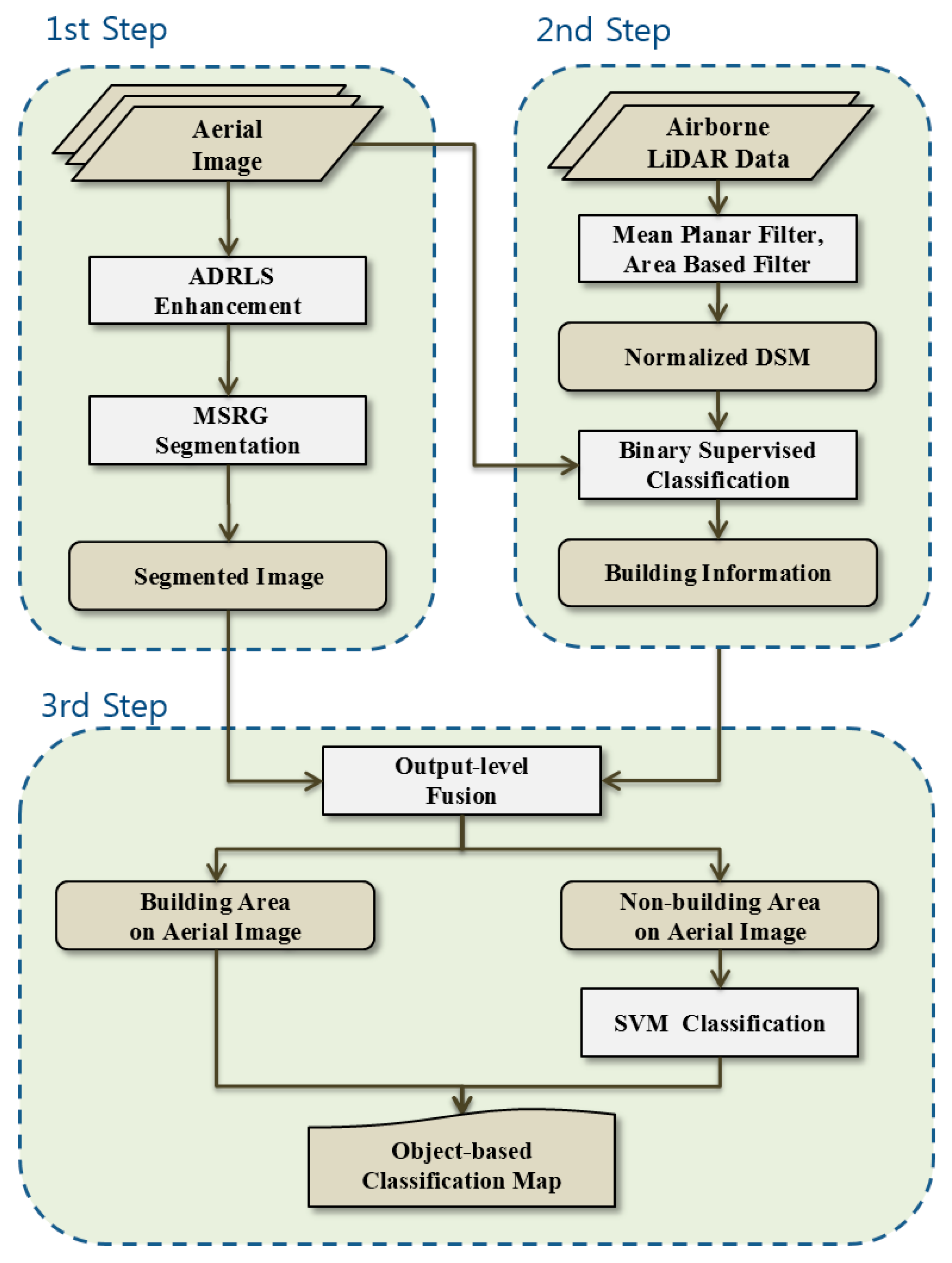
2. Materials and Methods

The new method is composed of the following three stages: image segmentation, building extraction, and classification after fusion. Figure 1 is a flowchart of the technique used to improve the classification accuracy through the fusion proposed in this study. The first step is to expand the image contrast by applying adaptive dynamic range linear stretching (ADRLS) image enhancement techniques to aerial images. Then, we apply a modified seeded region growing (MSRG) image segmentation technique to produce a segmented image. In the second step, a DTM is created by applying a mean planar filter (MPF) and an area-based filter (ABF) to the airborne LiDAR data, and a binary supervised classification is performed with the aerial image data to extract the building areas from the airborne LiDAR data. In the third step, buildings in the aerial images are extracted through the output-level fusion. Then, the SVM classification of non-building areas is conducted to generate the final object-based classification map. Finally, we select a comparison technique and perform a quantitative evaluation of the accuracy to verify the effectiveness of the new method.

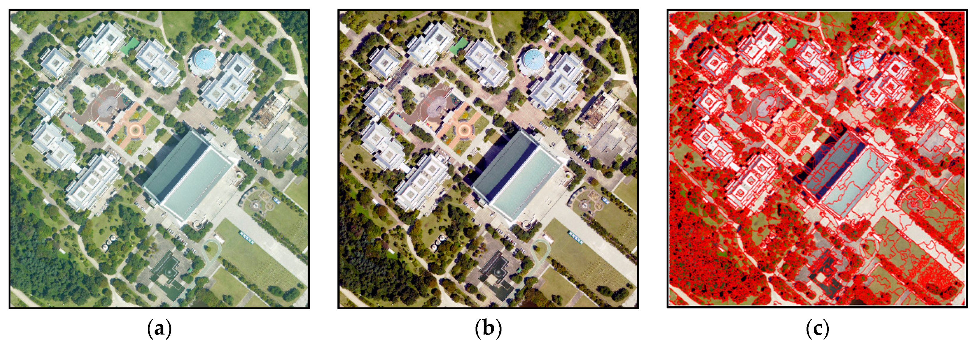
2.1. Image Segmentation of Aerial Image

2.1.1. Adaptive Dynamic Range Linear Stretching Image Enhancement

The histogram splitting technique proposed by Abdullah-Al-Wadud et al. (2007) [21] detects a local minimum in the histogram of an input image, and the section between two local minima with a normal distribution is generated in one of the sub-histograms. The local minimum is composed of the start value, end value, and the inflection point in the histogram. The histogram between two sub-local minima is reallocated in proportion to the number of pixels belonging to that range. The dynamic range relocation procedure of the sub-histogram is defined by Equation (1).

$$newrang{e}_i=\left(L-1\right)\times \frac{CD{F}_i}{CDF}$$

(1)

• L: radiometric resolution
• CDF: the total number of pixels in the sub-histogram
• CDF_i: the total number of pixels in the i-th sub-histogram

However, brightness values having a low frequency will have a relatively low contrast after the transformation because brightness values in the image with a high frequency occupy a large dynamic range in the conversion process. It is possible to minimize the dynamic range compression problem caused by the prevalence of the brightness values through the adaptive scale factor. The adaptive scale factor proposed by Park et al. (2008) [22] serves to readjust the dynamic range. The adjustment range of the theoretical sub-histogram r is defined by Equations (2) and (3). The adaptive scale factor has a range of (0, 1), and in this study, the value of the scale factor is set to a median of 0.5.

$$r=\frac{L}{k}$$

(2)

• L: radiometric resolution
• k: split value (the number of sub-histograms).

The dynamic range of the final sub-histogram is defined by Equation (3).

$$Finalrang{e}_i=newrang{e}_i+\mathsf{\alpha }\times \left(\mathrm{r}-newrang{e}_i\right)$$

(3)

• α: scale factor.

After the dynamic range of the sub-histograms is reset, a linear enhancement technique is applied to each sub-histogram unit. The linear enhancement technique is defined in Equation (4), as follows:

$$Y_n=f\left(x\right)=a{X}_n+b$$

(4)

• X_n: The n-th pixel brightness values of the input image histogram
• Y_n: Output pixel value of Xn
• a: Radiometric resolution/use range of the input image
• b: Horizontal translation variables

where a serves to extend the brightness range of the input image as the transformation coefficient, and b serves as a horizontal translation variable that is used to translate the output pixel value. Contrast of an image is increased through this image enhancement algorithm and separability between objects is improved in image segmentation because boundaries of the objects are clearer.

2.1.2. Modified Seeded Region Growing (MSRG)

The MSRG algorithm performs image processing using a multi-valued anisotropic diffusion technique that can improve the multi-spectral image while protecting the edge information. Then, the edge information, which integrates the band information of multi-spectral images, is extracted using an entropy-based edge detection operator proposed by Shiozaki (1986) [23]. The entropy measurement of a particular window mask region in a single band is defined in Equation (5).

$$E={\displaystyle \sum }_{i=1}^n{p}_i\frac{log{p}_i}{log\left(n+1\right)},p_i=\frac{a_i}{{{\displaystyle \sum }}_{j=1}^n{a}_j}$$

(5)

• n: total number of neighboring pixels;
• a_i: arbitrary pixel value in the window;
• a_j: represents the j-th neighboring pixel value where j = 1 to n;
• p_i: the ratio of an arbitrary pixel value over the summation of all pixel values

The integrated entropy measurements containing the contrast information of individual bands can be expressed as a linear combination of individual entropy measurements, as in Equation (6).

$$H={\displaystyle \sum }_{k=1}^N{q}_k{E}_k,q_k=b_k/{\displaystyle \sum }_{k=1}^N{b}_k$$

(6)

• N: total number of bands;
• q_k: the ratio of arbitrary pixel value over total pixel value;
• b_k: pixel value of the central pixel in the local window of the individual bands;
• E_k: entropy measure of the central pixel in the local window of the individual bands.

H takes on large values in edge regions and small values in low contrast regions within the range (0, 1). The local minimum is used to detect the seed point from these edge images. Each pixel locates another pixel with the lowest gradient among the neighboring pixels and moves in that direction. By repeatedly performing the same operation, a local minimum value is reached that cannot be further adjusted. This local minimum is the seed point. The difference between the detected local minimum values and the values of the eight directions around the adjacent points is calculated; if a lower value than the threshold is found, then the re-spreading process is conducted to locate the local minimum again.

The MSRG algorithm starts with the extracted seed point S₁, S₂, …, S_n, and attempts to aggregate the unlabeled pixels T to one of the given seed regions [24], as shown in Equation (7).

$$T=\left\{\left(x,y\right)\notin \underset{i=1}{\overset{n}{{\displaystyle \cup }}}{s}_i|N\left(x,y\right){\cap }^{\text{}}\underset{i=1}{\overset{n}{{\displaystyle \cup }}}{s}_i\ne \Phi \right\}$$

(7)

N(x, y): the set of nearest neighbor directions of 8 pixels for each area.

Individual elements of the set T are assigned to the nearest area for each step of the region growing process. The values of the function Ф(x, y) are sorted in ascending order to determine the similarity between all of the assigned elements and adjacent pixels, and then we select the priority of the region growing process in the next step. The similarity decision function using multispectral edge information is defined in Equation (8) where ‖‖ and • represent the vector norm and inner product, respectively.

$$\varphi \left(x,y\right)=\frac{\overrightarrow{c}\cdot \overrightarrow{p}}{{\Vert \overrightarrow{p}\Vert }^2}\times \left|G_c-G_p\right|$$

(8)

• $\overrightarrow{c}$: spectral vector of each region;
• $\overrightarrow{p}$: vector of adjacent neighboring pixel;
• G_c: the mean edge strength of each region;
• G_p: the edge magnitude of the multispectral edge map (H).

Figure 2 shows the results of applying the ADRLS and MSRG to obtain a high-resolution aerial image. The ADRLS image enhancement algorithm strengthened the contrast of the original image. The segmented image was produced by applying the MSRG algorithm.

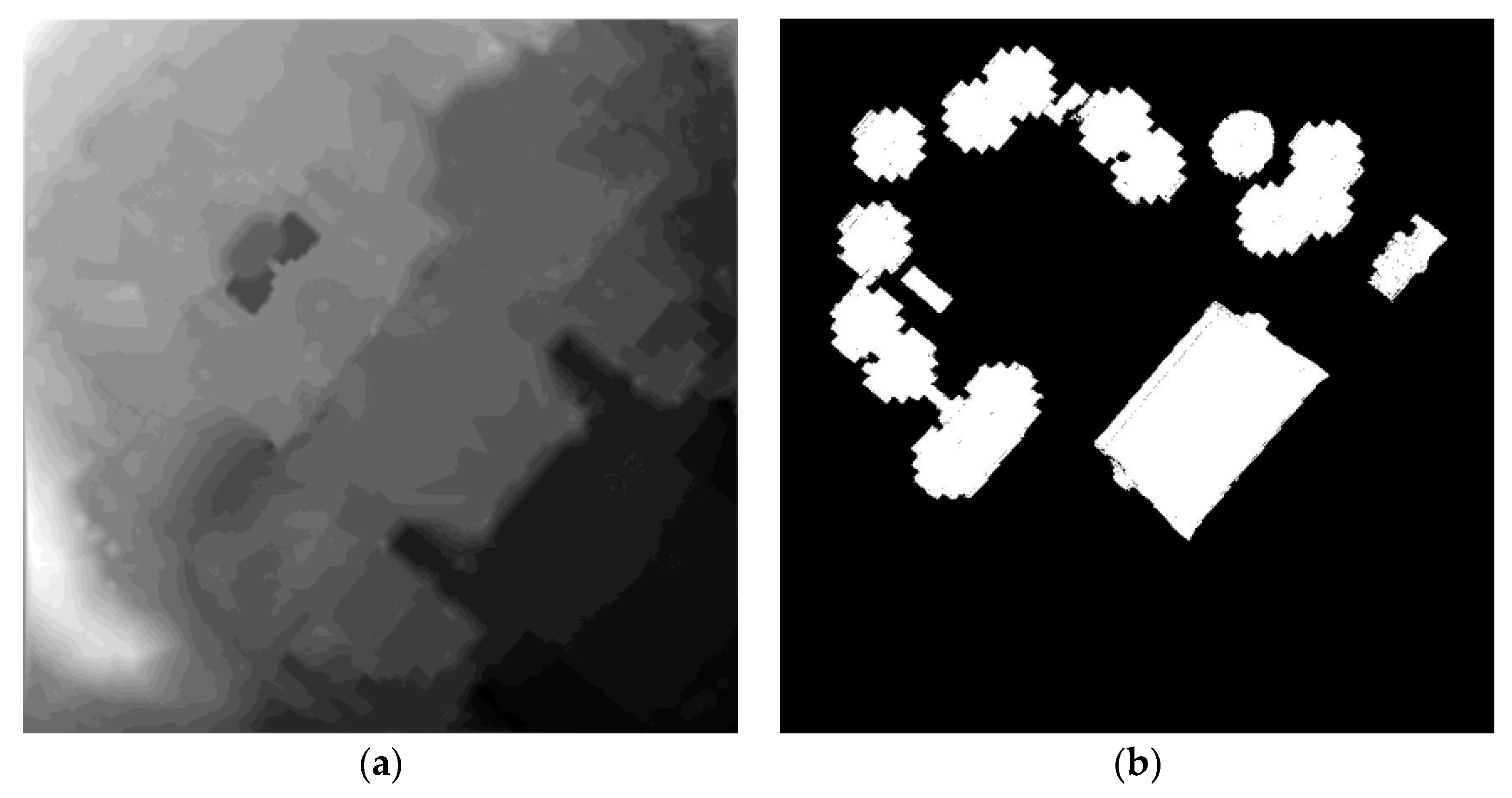
2.2. Extraction of Building Information from Airborne LiDAR Data

2.2.1. Generation of DTM

The pre-processing of airborne LiDAR data includes raster conversion and the removal of outliers. The airborne LiDAR data based on point clouds are rasterized for fusion with the optical data based on the raster, such as satellite images or aerial images. In this study, the point cloud data of the airborne LiDAR are transformed to raster data through the triangular irregular network (TIN) and nearest neighborhood interpolation for generating DSM (Digital Surface Model). Then, a histogram based on height values is used to find and remove outliers causing errors, such as negative values and positive values that are much higher than other values. The TIN interpolates the regularly distributed points as well as the irregularly distributed points; this network can reduce the data redundancy of the interpolation process for steep slopes and complicated terrains.

The Mean Planar Filter (MPF) segments the LiDAR data into planar surfaces and non-planar surfaces by detecting the boundary points using a simple 3 × 3 kernel. The MPF creates a mean plane with a size of 3 × 3 using nine height values, as in Equation (9). Then, the center of the kernel is defined as a non-planar pixel if there is at least one value whose distance from the mean plane is greater than a given threshold. This process is conducted across the entire image. The threshold is dependent on the size of the grid, and it is determined by the ratio of 5:3. For example, the threshold is set to 0.3 m for the case in which the grid size is 0.5 m [25].

$$M_{ij}=mean\left[\begin{array}{c}DSM\left(i-1,j-1\right),DSM\left(i-1,j\right),DSM\left(i-1,j+1\right),\\ DSM\left(i,j-1\right),DSM\left(i,j\right),DSM\left(i,j+1\right)\\ DSM\left(i+1,j-1\right),DSM\left(i+1,j\right),DSM\left(i+1,j+1\right)\end{array}\right]$$

(9)

• $M_{ij}$: mean plane created by the mean value of ${\text{kernel}}_{\text{ij}}$;
• $DS{M}_{ij}$: height value of location (i, j).

Planar surfaces extracted by the MPF include ground points as well as the flat roofs of a building. Therefore, planar surfaces composed of a flat roof should be removed to extract only the ground points. The ABF algorithm proposed by Ma (2005) [26] can be used to solve this problem. The ABF algorithm using the area of the largest roof segment in the segmented image, extracts the segment composed of only the ground points by removing the flat segment having a smaller area than the largest roof segment. The largest roof segment is selected manually in the segmented image. The ABF algorithm can effectively perform the extraction process for ground points because ground points with connectivity have a large surface area relative to other objects in the binary image segmentation. Therefore, only ground points are extracted. A temporary DTM is generated using these ground points.

Refinement of the DTM involves repeatedly comparing the DSM with the temporary DTM generated in the previous step. This process repeatedly generates an accurate and detailed DTM with additional detected ground points when the height difference between the DSM and the temporary DTM is less than 0.3 m. The threshold difference is based on the vertical accuracy (±0.15 m) of LiDAR, and there is only a slight change in the ground points after three repetitions of the refinement process. Details of the refinement can be found in [26].

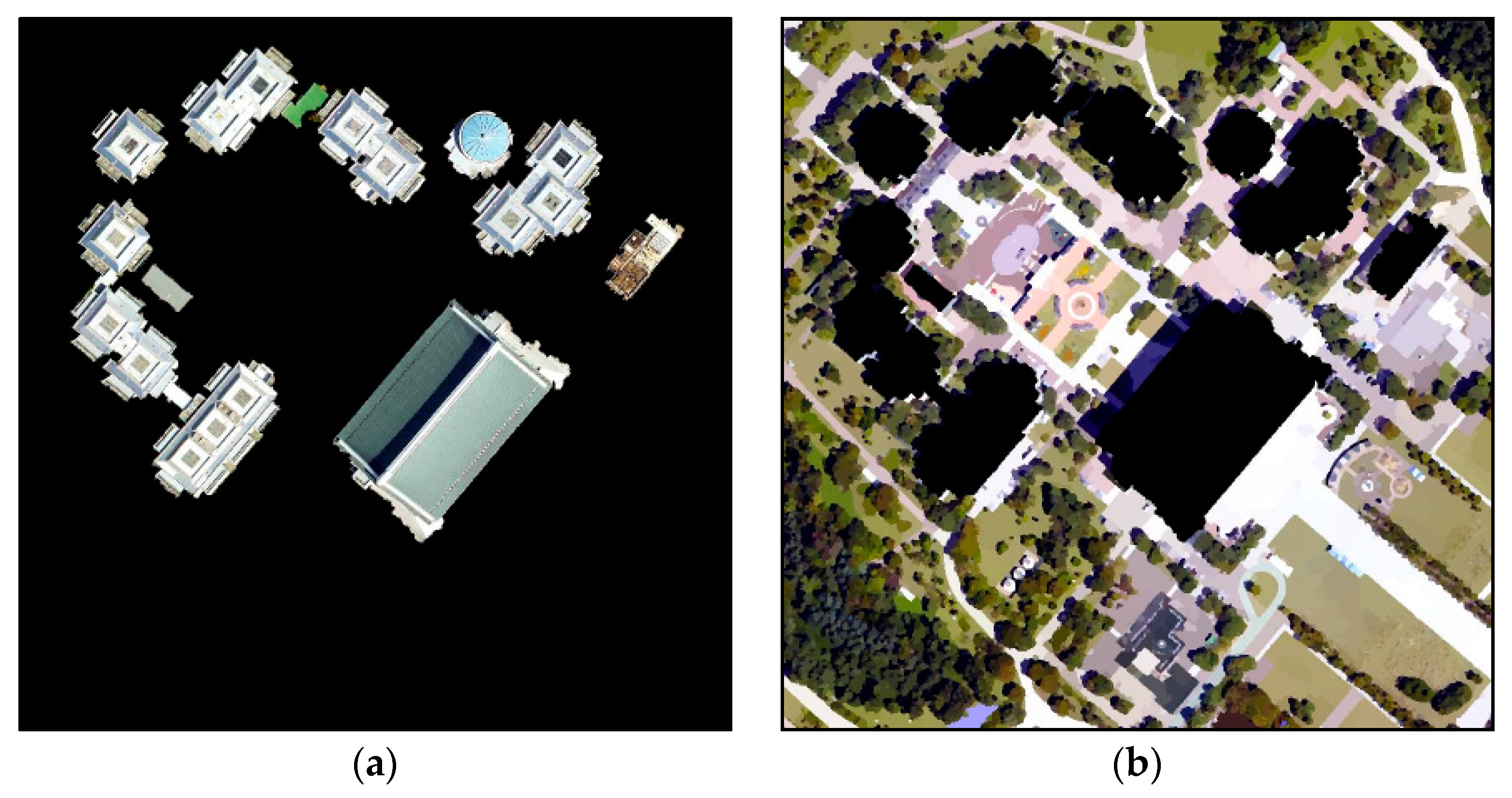
2.2.2. Building Detection

nDSM can be created by subtracting a DTM from a DSM, giving the height of the object from the ground [27]. Tall objects, such as buildings and trees, in airborne LiDAR data can be extracted by applying a threshold to the nDSM. Regardless of the shape and spectral properties of the building roof, this process has the advantage that it can be applied easily because it uses only the height element of an object. The height threshold in this study is set to 2 m, the minimum height of a building, and the process extracts all objects having a height that is greater than the threshold. These extracted objects include buildings, tree canopies, and various facilities. Therefore, it is necessary to remove non-building objects to detect only building objects. To extract the buildings, binary supervised classification with aerial images and nDSM provides a good performance.

The following three processes are a prerequisite for binary supervised classification using SVM:

1

Perform supervised classification only for areas with tall objects

2

Use nDSM as an additional band to the RGB bands of aerial images

3

Classify into vegetation and non-vegetation

The binary supervised classification process uses only areas with the tallest objects, rather than using the full area of the aerial image. Thus, if only areas with tall objects are used to perform supervised classification, misclassification between objects, such as trees and grass, having similar spectral characteristics is decreased. Further, in the classification process, the separability between vegetation and non-vegetation is improved using nDSM because objects having similar spectral characteristics with different heights remain [28,29]. Building objects and small objects, such as a bench and sculpture, remain after removing the vegetation area in the results of binary supervised classification. Finally, the threshold is set to 60 m² as a minimum criterion of the residential area, and the ABF algorithm is performed [30]. Objects with an area that is smaller than the threshold are removed through the ABF, and the remaining building objects in the airborne LiDAR data are extracted. Figure 3 shows building information extracted from the airborne LiDAR data and aerial images through the new method.

2.3. Output-Level Fusion and Generation of Classification Maps

Segmented aerial images generated by the MSRG algorithm are composed of many segments surrounded by boundaries not only between different objects but also within an object. Therefore, it is necessary to extract segments consisting of the building objects from the aerial image. Output-level fusion plays a role in extracting the building segments from aerial images using building information from airborne LiDAR data along with segment information from aerial images. The output-level fusion proposed in this study does not require merging and matching processes to extract building objects. Additionally, it can obtain more detailed and accurate areas compared with the building area obtained using a simple overlay of the aerial image and airborne LiDAR data. The fusion process is conducted using Equation (10). After overlaying the segments of the aerial image and the building area of the airborne LiDAR data, the process calculates a ratio of the area occupied by buildings in the airborne LiDAR data within each segment of the aerial image. The empirical threshold used to minimize the commission error determines whether the segment is a building. If the ratio is greater than 50%, then the segment is a building segment [31]. A number of building segments extracted by the output-level fusion is reconstructed into a building by applying closing operations in the morphology filter.

$$\{\begin{array}{c}Ro{S}_i=\frac{Buildingarea}{Segmen{t}_i}\\ IfRo{S}_i\ge 0.5,Segmen{t}_i=Buildingsegment\end{array}$$

(10)

• RoS_i: ratio of the building area overlaid on the i-th segment;
• Building area: building area overlaid on the i-th segment;
• Segment_i: i-th segment area.

Building information extracted through the output-level fusion is used as a priori information for the classification of aerial images. This can prevent misclassification caused by objects having spectral characteristics similar to the building or the building having different spectral properties by assigning previous building objects to the building class of the aerial image. The classification process is applied to objects in the remaining region other than the pre-extracted building region. The segmentation process applied to the aerial image does not need to be repeated because the segment region used is the same as that of the segmented aerial image. Bands used for the classification are the nDSM and RGB bands of the aerial image, and a SVM is used as a classifier. The final classification map is generated by combining the object-based classification results for non-building areas and the building class previously assigned. Figure 4 shows the building area and the non-building area on the aerial image derived from the output-level fusion of the aerial image and airborne LiDAR data.

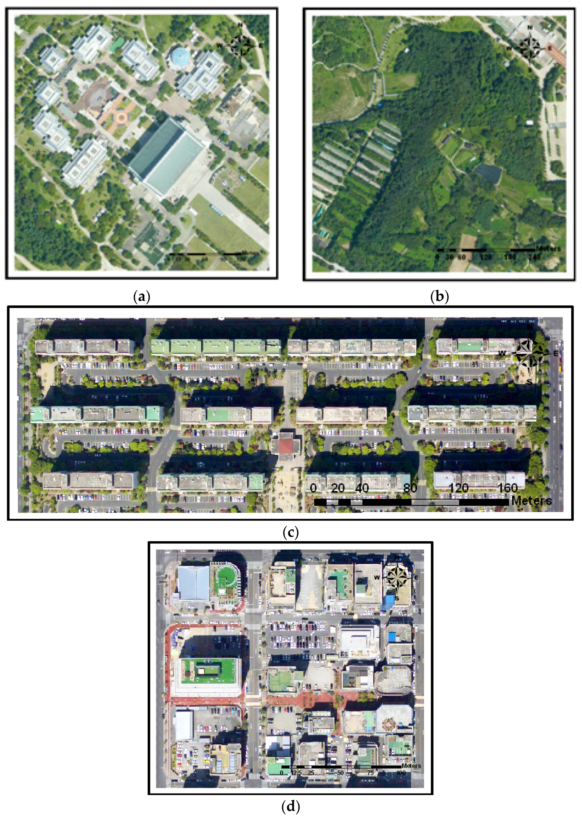
3. Data Used and Experimental Sites

The aerial image used in this study was acquired in May 2005 (sites 3 and 4) and September 2009 (sites 1 and 2) using a Digital Mapping Camera. The image includes red, green, and blue bands of the visible region and has a spatial resolution of 0.25 m. Airborne LiDAR data were acquired using an Optech ALTM 3070, and the point density was 4.3 points/m². They were acquired together, and the aerial image was ortho-rectified.

Experimental sites 1 and 2 have characteristics of urban and forest land cover near Independence Hall in Cheonan, South Korea (36°47′1′′N, 127°13′22′′E). They are composed of a number of large buildings, forests, and grasslands, and the spectral properties of the building roofs and the roads are similar. Thus, the sites are suitable for evaluating the performance of the new method for objects having similar spectral properties, such as roads and buildings. Experimental sites 3 and 4 are in Daejeon, South Korea (36°21′4′′N, 127°23′25′′E), and most of the area is composed of land covers that characterize urban environments, such as concrete and asphalt.

Table 1. Characteristics of experimental sites.

Site	Coverage	Range of Height	Characteristics
1	425 × 425 m	0~58.8 m	Mixed area
2	625 × 625 m	0~63.4 m	Mixed area
3	450 × 160 m	0~53.2 m	Apartment area
4	200 × 225 m	0~74.1 m	Building area

summarizes the characteristics of each site, and Figure 5 shows their coverage through aerial images.

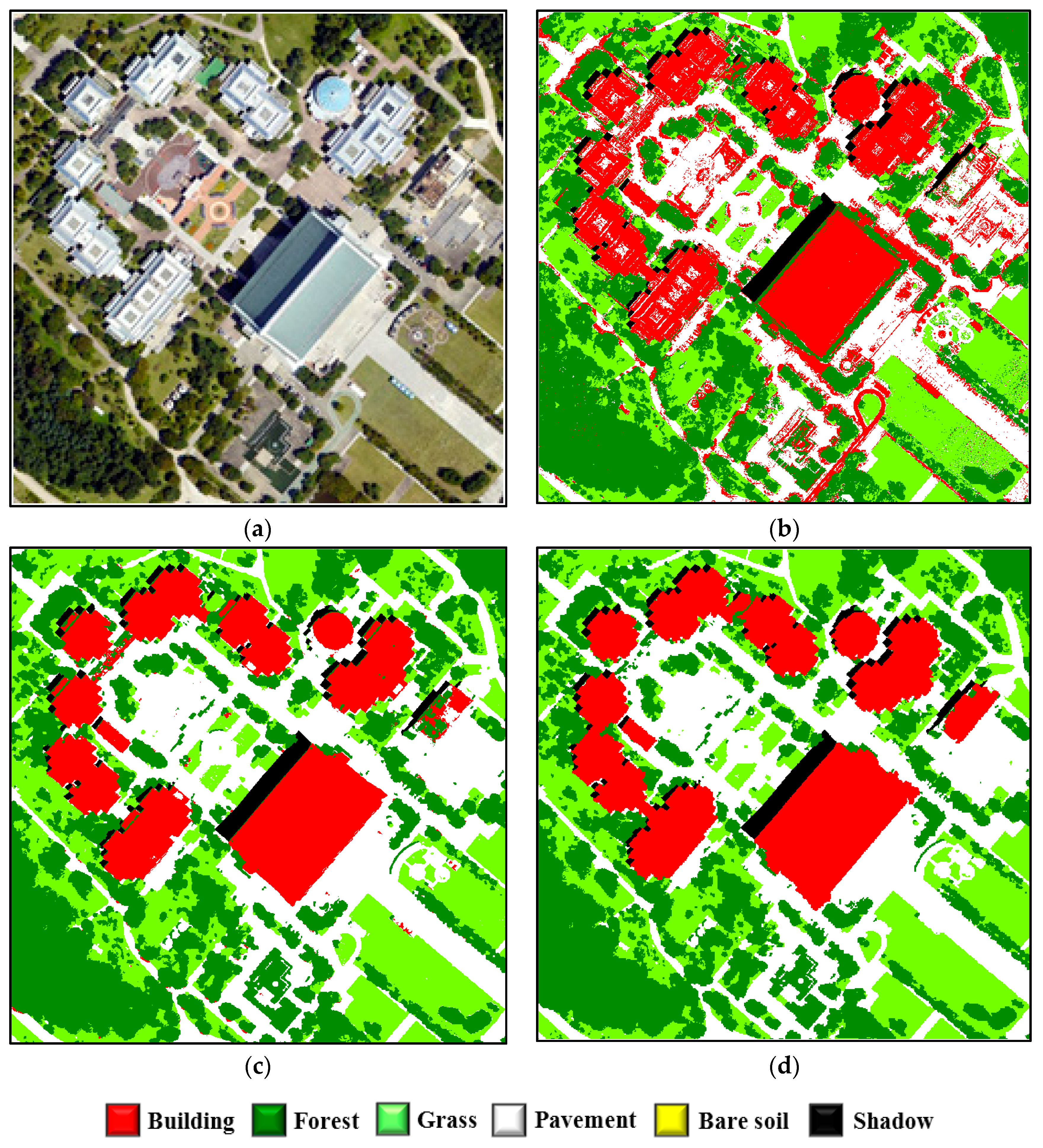
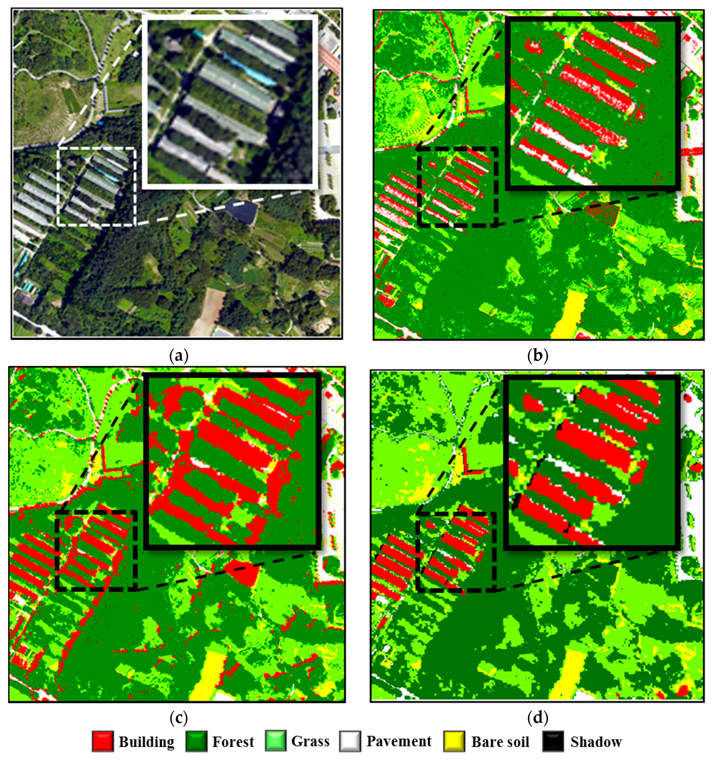
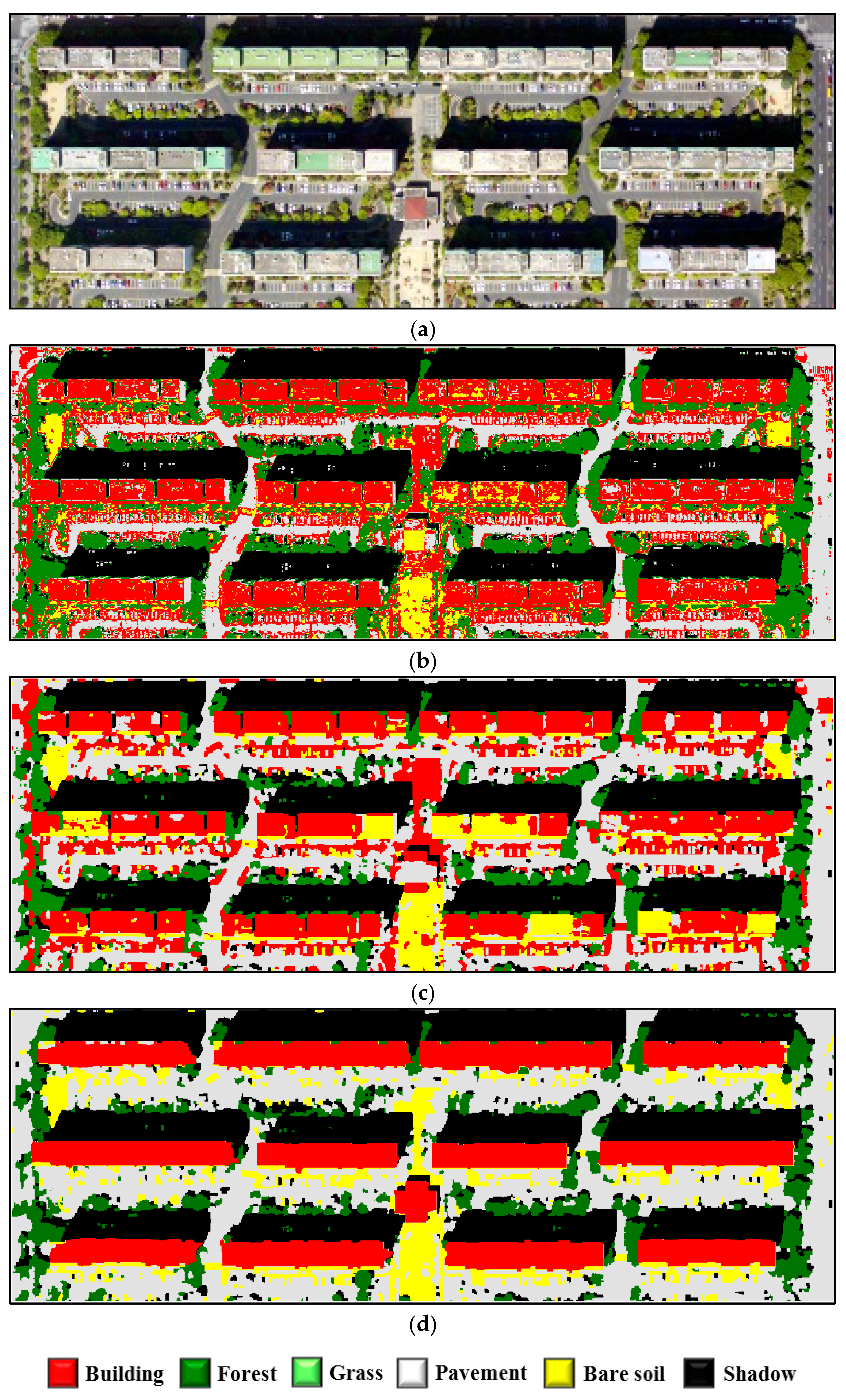
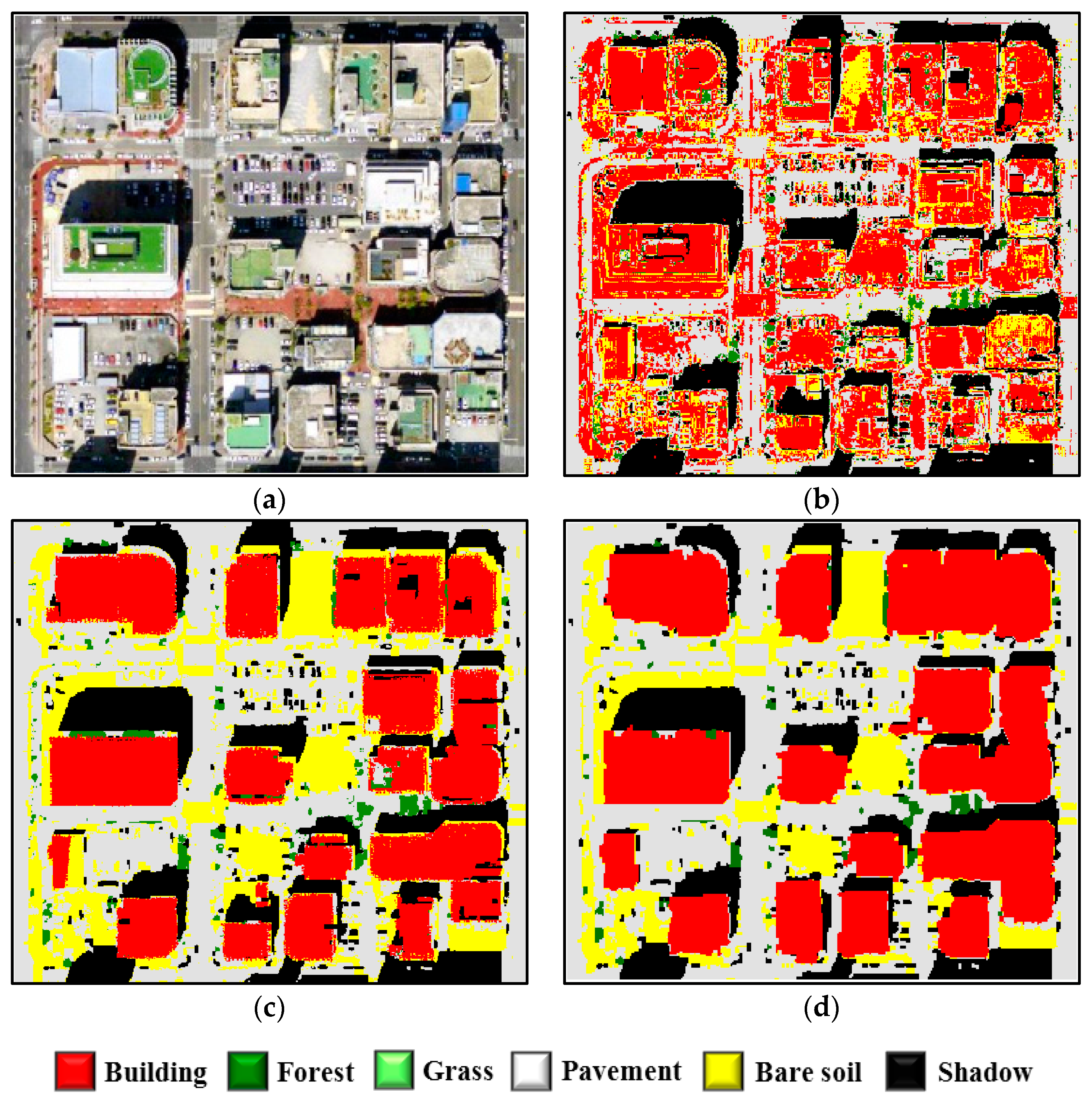
4. Results and Discussion

4.1. Methods for Comparison

Huang (2011) et al. [20] conducted a study to derive the optimal classification results by applying various fusion techniques for aerial images and airborne LiDAR data. The classification results were obtained by feature-level, output-level, and decision-level fusion using the height difference, the variance of the height difference, and GLCM extracted from airborne LiDAR data. The classification results of the Max-Min output-level fusion showed the highest accuracy for many results, and the size of the utilized filter was 13 × 13, with a spatial resolution of 0.4 m. However, in this study, to compare the methods under similar conditions, an 11 × 11 filter was applied to the four experimental areas, considering the spatial resolution of the aerial image.

In contrast to the existing methods that specify the initial seed point, the region growing method proposed by Han et al. (2012) [17] sequentially assigns the initial seed point for all of the pixels. The SSI of the segments extracted through the region growing method serves to improve the separability between the building and road objects. The SSI is defined by Equation (11), as follows:

$$SSI=\frac{Perimeter}{Are{a}^w},\left(w\ge 0\right)$$

(11)

where Perimeter is the perimeter of a segment, Area is the area of a segment, and w is the weight.

The greater the weight w is, the greater is the influence of the area on the classification result. In this study, the similarity parameter was set to 30, and the weight parameter was set to 1 through the tests with different parameters. For comparison under the same conditions, the same segment areas were used in the classification process. In addition to the red, green, and blue bands of the aerial image, SSI and nDSM were used in the SVM supervised classification as an additional band.

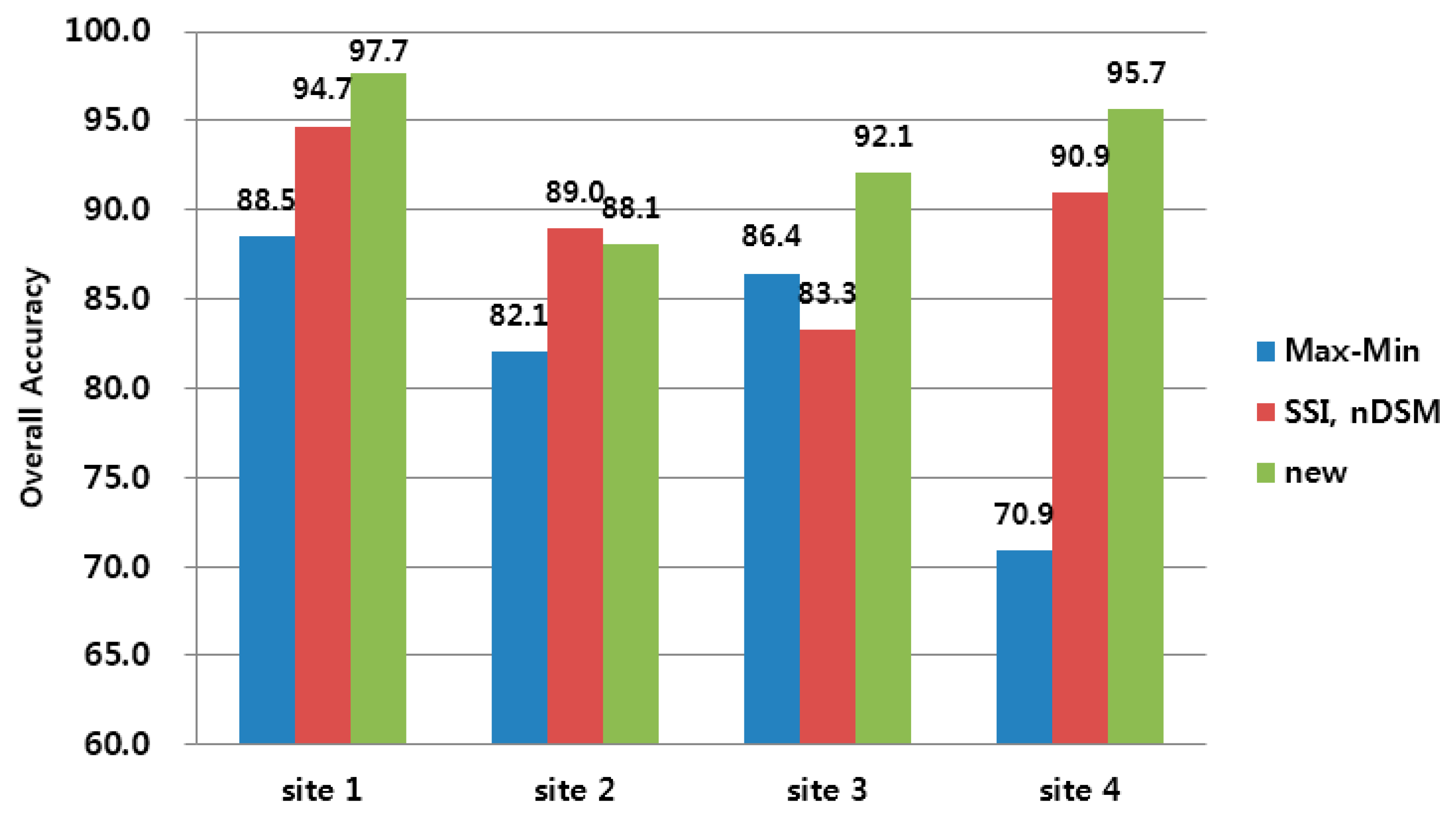
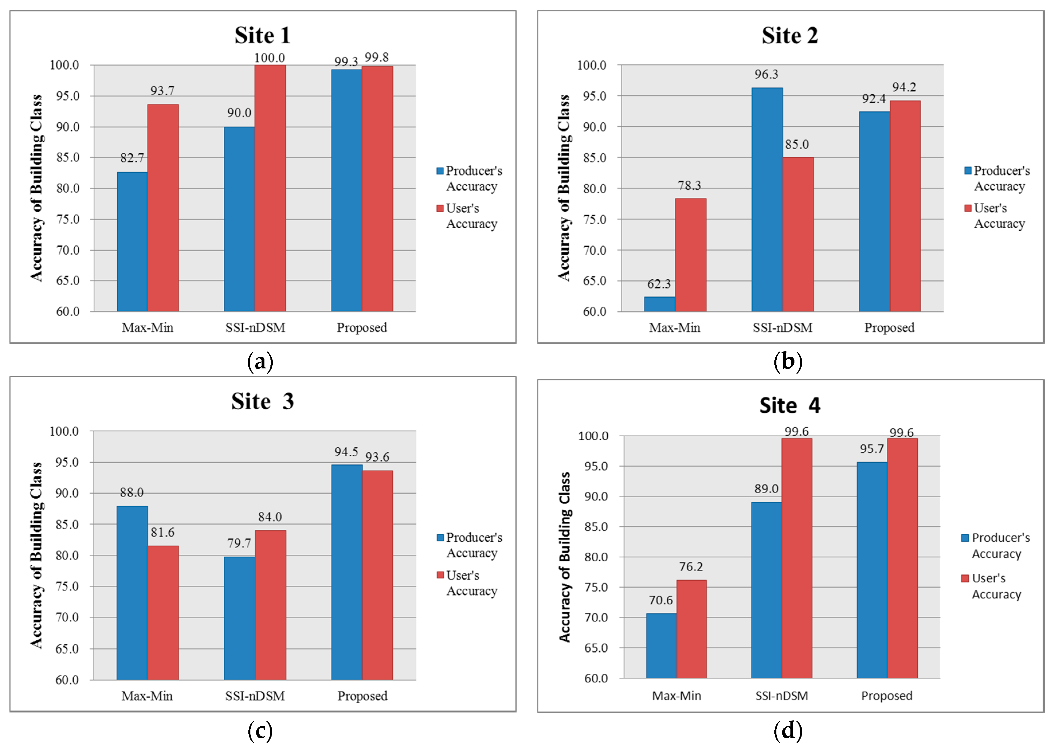
4.2. Accuracy Assessment

The final classification results of the new method and the compared methods for site 1 can be observed in Figure 6. For the Max-Min classification method in Figure 6b, the use of the height value in the airborne LiDAR data improved the separability between pavement and building objects and increased the classification accuracy. However, there are misclassifications between the building roof surface and pavement pixels resulting from the pixel-based classification method. Further, the buildings on the right side of the site were classified as the pavement class. In the object-based classification using SSI-nDSM, the salt-and-pepper noise that occurred in the classification results produced by the Max-Min method did not occur in the object-based classification. Therefore, it is visually confirmed that the classification accuracy of the building class is improved in Figure 6c. However, misclassifications of building objects on the right side of the site also occurred in the results using the SSI and nDSM together. In the case of the new method of Figure 6d, problems that occurred using the comparative evaluation methods were solved using the object-based classification and the building information extracted from airborne LiDAR data.

The results of the new method and the comparative methods for site 2 can be found in Figure 7. For site 2, misclassifications between building and pavement objects originated from the classification results of the Max-Min process, similar to site 1. The building located to the left of site 2 was misclassified as the pavement class, and the pavement located at the top was misclassified as the building class. In the object-based classification results using SSI and nDSM, the separability between building and pavement and forest and grass was improved, and misclassifications were significantly reduced compared with the results using the Max-Min method. However, the results contained many errors for the building class, e.g., a black ginseng field located at the center of the site was misclassified as the building class. This is because a black ginseng field with similar spectral characteristics was recognized in the same building object because of using the roof surface of the navy as training data for the building object. This result might be a good example of reducing the separability if the height between different objects is similar, even though the SSI and nDSM are used as an additional band. However, the new method showed the results of improving the misclassification accuracy between building and pavement objects by classifying the building objects in advance. Additionally, misclassification between forest and grass objects was significantly reduced. However, we observed an error in which the bare soil object is classified as the building class on the bottom right of the site. We confirmed that the distortion generated during DTM generation propagates to the building detection process, and the errors affect the final classification results.

The classification results for site 3, consisting of apartment buildings, are shown in Figure 8. Site 3 shows misclassification between building and pavement objects having similar spectral characteristics because there are many roof surfaces composed of concrete compared with the other sites. Although the Max-Min method in Figure 8b is a pixel-based algorithm, it was confirmed that apartment objects are well classified as the building class. However, we observe a problem in which the pavement objects are misclassified as the building class. In the object-based classification results using SSI and nDSM shown in Figure 8c, omission errors in which an apartment roof was classified as the bare soil class were found more often in site 3 than in sites 1 and 2, possibly because of similar SSIs at site 3. When using the new method, the objects are correctly extracted, although small omission errors of the apartment located on the left side were observed. This can be confirmed by Figure 8d as an effect of output-level fusion.

The results for objects in site 4, having similar spectral characteristics, such as for building roof surfaces and road surfaces, can be observed in Figure 9. The classification results using the Max-Min method produced errors between building and pavement objects and provided a low classification performance. The method using SSI and nDSM effectively reduced the occurrence of misclassifications among the building, pavement, and concrete objects using the Max-Min method. However, omission errors occurred in which certain buildings were classified as the bare soil class, and building roof surfaces in shadows were classified as the shadow class. The new method demonstrated a benefit because it is not affected by shadows, although a building boundary that is not properly extracted in the segmentation process when applied to the aerial image causes missing errors. Vehicles on the ground were observed due to the high spatial resolution of the aerial image, and black vehicles were classified as shadows.

Taken together, the new method does not require the process of acquiring training data for each of the building roof colors, unlike comparative methods, because building objects were previously assigned. Additionally, the method provides an advantage that it reduces commission errors of other classes and generates high-quality classification results. Specifically, it has the effect of considerably reducing the misclassification of building and pavement objects. It was confirmed that the separability of objects having similar spectral properties is further improved using nDSM at the four experimental sites.

To conduct a quantitative assessment, reference data were obtained for building, pavement, forest, grass, and bare soil land types from aerial images as point types. We obtained 1455 points in site 1, 1863 points in site 2, 582 points in site 3, and 522 points in site 4 through the random sampling method. Then, the overall accuracy was calculated by configuring the confusion matrix for a comparison of the classification results. Figure 10 shows the overall accuracy of the classification results when applying the three classification techniques to the four experimental areas in the graph, and

Table 2. Improved accuracies of the new method over the other methods.

	Max-Min (%)	SSI-nDSM (%)
Site 1	9.2	3
Site 2	6	−0.9
Site 3	5.7	8.8
Site 4	24.8	4.8

summarizes the measurements of the improved overall accuracy obtained using the new method.

In site 1, the new method achieved additional accuracy improvements of 3% and 9.2% over the compared methods. The classification results using the Max-Min method included many misclassifications between buildings and pavement or forests and grasslands, which led to a decreased overall accuracy, while the classification results using SSI and the new method exhibited a high classification accuracy for all of the classes. Although the new method showed an improvement of 6% compared with the accuracy of the Max-min method for site 2, it provided a 0.9% lower accuracy than the classification using nDSM and SSI. The new method caused an error in which the bare soil located on the bottom right was detected as a building area in the building detection process, reducing the accuracy of the final producer for building class detection. In the Max-Min results, misclassifications between building and pavement objects in site 1 were not observed. The three methods applied to site 2 exhibited a lower accuracy compared with the other three sites because of site 2’s characteristics. This is because site 2 is primarily composed of a tree canopy and grass objects having similar spectral information, and the accuracy of the DTM generation and building detection processes is reduced in areas next to building and tree canopy objects. In site 3, the SSI and nDSM method produced misclassifications between apartment roof and bare soil objects and building and pavement objects, in contrast to sites 1 and 2. The Max-Min method exhibited a problem in which a parking line was classified as the building class, and the accuracy of the building class is higher than that for other sites. The new method had increased accuracies of 5.7% and 8.8% over the Max-Min and SSI-nDSM methods, respectively, because it effectively decreases misclassifications between building and pavement objects in the classification process through the previous assignment of the building class. In site 4, the Min-Max method provided a lower accuracy compared with the other two methods, indicating that the separability between building and pavement objects with similar spectral characteristics is not markedly improved using the Max-Min method. The SSI-nDSM method exhibited a problem in which a shadow object on a building roof was not classified as either the building class or the shadow class. This is because the spectral characteristics of the shadow affected the classification process more strongly than did the SSI and nDSM characteristics of the pixels. However, the new method has an advantage whereby the problem caused by the shadow is not observed because this method uses the building information extracted from airborne LiDAR data. The new method showed a slightly lower accuracy for the asphalt class, but it provides a higher classification accuracy than that provided by comparable methods for other classes. Additionally, the new method showed improved accuracies of 24.8% and 4.8% over the Max-Min and SSI-nDSM methods, respectively.

The producer’s and user’s accuracies for the building class are shown in the graph in Figure 11. A key point of this study is to improve the overall accuracy by mitigating the misclassification of building objects. The improved value was calculated using the average value of the producer’s and user’s accuracies. The results of the new method showed classification accuracies higher than 90% at all of the experimental sites. It improved the accuracy from 9.31% to 24.26% over the Max-Min method and from 4.55% to 12.4% over the SSI-nDSM method, indicating that the Max-Min method cannot effectively use the height information of airborne LiDAR data for the experimental sites. The SSI-nDSM method has an accuracy that is similar to that of the new method for the building class, except for the misclassifications as bare soil in site 3. The new method improved the classification accuracy by solving the misclassification problem among building, pavement, and shadow objects in the classification process by performing output-level fusion.

When analyzing the tendencies of the accuracies in Figure 10 and Figure 11, we can confirm that the total and building accuracies have a high correlation. This indicates that the classification accuracy for buildings had a significant effect on the overall accuracy, which is more evident in areas with urban characteristics, such as sites 3 and 4. Specifically, in the classification of high-resolution optical images, the accuracy for building objects directly affects the overall accuracy. Particularly, it greatly affects the quality of the classification in the case of urban environments, which primarily include building objects.

Consequently, the new method showed good performance in the quantitative accuracy assessment, especially in terms of its strong ability to improve the accuracy by pre-assigning the building objects. However, it is necessary to consider the following points when applying the new method. First, the new method exhibits a good performance in urban areas, where buildings are often densely distributed, whereas its effect is limited in forest areas and sub-urban areas that include sparse distributions of buildings because the new method improves the classification accuracy by pre-assigning the building class. Second, as observed in the final classification result, errors that occur in the DTM generation, building detection, and output-level fusion processes can affect subsequent steps. They continuously propagate and affect the final object-based classification results. Finally, objects such as automobiles, sculptures, and benches in the high-resolution aerial images used in this study have been identified. These objects can be generated with an error that is assigned to any category. Therefore, it is necessary to consider an “assign them to any class” category. For example, this can be determined by a majority filter that can be used as a replacement for the major class surrounding the objects.

5. Conclusions

High-resolution optical images suffer from a problem in which different objects have similar spectral characteristics or the same object has different spectral characteristics. These problems are more severe in urban environments and are exhibited most prominently by building objects. This study, through the output-level fusion of data, presents an attempt to solve these problems by minimizing the misclassification of building objects in high-resolution optical images. Therefore, the problems caused by various spectral characteristics of building objects were addressed by applying information about the building extracted from the airborne LiDAR data, which provides three-dimensional information to the classification process that is applied to the aerial image.

The output-level-fusion-based classification method for aerial images and airborne LiDAR data proposed in this study was applied to four experimental sites, and a comparative evaluation with the Max-Min method and the SSI-nDSM method was performed. The new method, the Max-Min method, and the SSI-nDSM method showed high precision, and the new method was found to improve the overall accuracy typically by more than 5% compared with the comparative evaluation methods. Additionally, the high and low patterns exhibited by the overall and building accuracies were similar. This strengthens the theory that the classification accuracy of buildings has a significant effect on the overall accuracy, which is more evident in areas with urban characteristics.

This study confirmed that the additional use of airborne LiDAR data is effective for the classification of high-resolution optical images; particularly, it contributes to increasing the overall accuracy and the accuracy of building classification. However, certain problems, such as the decrease in DTM accuracy for mixed land cover areas and class allocation of small objects, were identified. Therefore, we plan to conduct research to solve these problems in the future.

References

1. Rashed, T.; Jurgens, C. Remote Sensing of Urban and Suburban Areas; Springer: Dordrecht, The Netherlands, 2010. [Google Scholar]
2. Zhao, W.; Cheng, L.; Tong, L.; Liu, Y.; Li, M. Robust segmentation of building points from airborne LIDAR data and imagery. In Proceedings of the 19th International Conference on Geoinformatics, Shanghai, China, 24–26 June 2011.
3. Hall, D.L.; Llinas, J. An introduction to multisensory data fusion. IEEE Proc. 1997, 85, 6–23. [Google Scholar] [CrossRef]
4. Haala, N.; Brenner, C. Extraction of buildings and trees in urban environments. ISPRS J. Photogramm. Eng. Remote Sens. 1999, 54, 130–137. [Google Scholar] [CrossRef]
5. Lee, D.S.; Shan, J. Combining lidar elevation data and IKONOS multispectral imagery for coastal classification mapping. Mar. Geod. 2003, 26, 117–127. [Google Scholar] [CrossRef]
6. Dalponte, M.; Bruzzone, L.; Gianelle, D. Fusion of hyperspectral and LIDAR remote sensing data for classification of complex forest areas. IEEE Trans. Geosci. Remote Sens. 2008, 46, 1416–1427. [Google Scholar] [CrossRef]
7. Geerling, G.W.; Labrador-Garcia, M.; Clevers, J.G.P.W.; Ragas, A.M.J.; Smits, A.J.M. Classification of Floodplain Vegetation by Data Fusion of Spectral (CASI) and LiDAR Data. Int. J. Remote Sens. 2007, 28, 4263–4284. [Google Scholar] [CrossRef]
8. Schenk, T.; Csathó, B. Fusion of LIDAR data and aerial imagery for a more complete surface description. Int. Archives Photogramm. Remote Sens. Spat. Inf. Sci. 2002, 34, 310–317. [Google Scholar]
9. Hill, R.A.; Thomson, A.G. Mapping woodland species composition and structure using airborne spectral and LiDAR data. Int. J. Remote Sens. 2005, 26, 3763–3779. [Google Scholar] [CrossRef]
10. Rottensteiner, F.; Trinder, J.; Clode, S.; Kubik, K. Using the Dempster–Shafer method for the fusion of LIDAR data and multi-spectral images for building detection. Inf. Fusion 2005, 6, 283–300. [Google Scholar] [CrossRef]
11. Erdody, T.; Moskal, L.M. Fusion of LiDAR and Imagery for Estimating Forest Canopy Fuels. Remote Sens. Environ. 2010, 114, 725–737. [Google Scholar] [CrossRef]
12. Holmgren, J.; Persson, Å.; Söderman, U. Species identification of individual trees by combining high resolution LiDAR data with multi-spectral images. Int. J. Remote Sens. 2008, 29, 1537–1552. [Google Scholar] [CrossRef]
13. Kim, Y.M.; Chang, A.J.; Kim, Y.I. Extraction of building boundary on aerial image using segmentation and overlaying algorithm. J. Korean Soc. Surv. Geod. Photogramm. Cartogr. 2012, 30, 49–58. [Google Scholar] [CrossRef]
14. Zhan, Q.; Molenaar, M.; Tempfli, K. Hierarchical image object-based structural analysis toward urban land use classification using high-resolution imagery and airborne LIDAR data. In Proceedings of the 3rd International Conference on Remote Sensing of Urban Areas, Istanbul, Turkey, 11–13 June 2002; pp. 11–13.
15. Chen, Y.; Su, W.; Li, J.; Sun, Z. Hierarchical object oriented classification using very high resolution imagery and LIDAR data over urban areas. Adv. Space Res. 2009, 43, 1101–1110. [Google Scholar] [CrossRef]
16. Yeom, J.H.; Lee, J.H.; Kim, D.J.; Kim, Y.I. Hierarchical land cover classification using IKONOS and AIRSAR images. Korean J. Remote Sens. 2011, 37, 435–444. [Google Scholar] [CrossRef]
17. Han, Y.; Kim, H.; Choi, J.; Kim, Y. A shape-size index extraction for classification of high resolution multispectral satellite images. Int. J. Remote Sens. 2012, 33, 1682–1700. [Google Scholar] [CrossRef]
18. Hodgson, M.E.; Jensen, J.R.; Tullis, J.A.; Riordan, K.D.; Archer, C.M. Synergistic use of lidar and color aerial photography for mapping urban parcel imperviousness. Photogramm. Eng. Remote Sens. 2003, 69, 973–980. [Google Scholar] [CrossRef]
19. Nordkvist, K.; Granholm, A.H.; Holmgren, J.; Olsson, H.; Nilsson, M. Combining optical satellite data and airborne laser scanner data for vegetation classification. Remote Sens. Lett. 2012, 3, 393–401. [Google Scholar] [CrossRef]
20. Huang, X.; Zhang, L.; Gong, W. Information fusion of aerial images and LIDAR data in urban areas: Vector-stacking, re-classification and post-processing approaches. Int. J. Remote Sens. 2011, 32, 69–84. [Google Scholar] [CrossRef]
21. Abdullah-Al-Wadud, M.; Kabir, M.H.; Dewan, M.A.A.; Chae, O. A dynamic histogram equalization for image contrast enhancement. IEEE Trans. Consum. Electron. 2007, 53, 593–600. [Google Scholar] [CrossRef]
22. Park, G.H.; Cho, H.H.; Choi, M.R. A contrast enhancement method using dynamic range separate histogram equalization. IEEE Trans. Consum. Electron. 2008, 54, 1981–1987. [Google Scholar] [CrossRef]
23. Shiozaki, A. Edge extraction using entropy operator. Comput. Vis. Graph. Image Process. 1986, 36, 1–9. [Google Scholar] [CrossRef]
24. Byun, Y.; Kim, D.; Lee, J.; Kim, Y. A framework for the segmentation of high-resolution satellite imagery using modified seeded-region growing and region merging. Int. J. Remote Sens. 2011, 32, 4589–4609. [Google Scholar] [CrossRef]
25. Kim, Y.M.; Eo, Y.D.; Chang, A.J.; Kim, Y.I. Generation of a DTM and building detection based on an MPF through integrating airborne lidar data and aerial images. Int. J. Remote Sens. 2013, 34, 2947–2968. [Google Scholar] [CrossRef]
26. Ma, R. DEM Generation and Building Detection from LiDAR Data. Photogramm. Eng. Remote Sens. 2005, 71, 847–854. [Google Scholar] [CrossRef]
27. Koch, B.; Straub, C.; Dees, M.; Wang, Y.; Weinacker, H. Airborne laser data for stand delineation and information extraction. Int. J. Remote Sens. 2009, 30, 935–963. [Google Scholar] [CrossRef]
28. Arroyo, L.A.; Johansen, K.; Armston, J.; Phinn, S. Integration of LiDAR and QuickBird imagery for mapping riparian biophysical parameters and land cover types in Australian tropical savannas. For. Ecol. Manag. 2010, 259, 598–606. [Google Scholar] [CrossRef]
29. Chadwick, J. Integrated LiDAR and IKONOS multispectral imagery for mapping mangrove distribution and physical properties. Int. J. Remote Sens. 2011, 32, 6765–6781. [Google Scholar] [CrossRef]
30. Committee of Codification of Law. Limit of Building Area; Ministry of Land, Infrastructure, and Transport: Sejong-si, Republic of Korea, 2011.
31. Kim, Y.M.; Kim, Y.I. Improved classification accuracy based on the output-level fusion of high-resolution satellite images and airborne LiDAR data in urban area. IEEE Geosci. Remote Sens. Lett. 2014, 11, 636–640. [Google Scholar]
Figure 1. Flowchart of classification generation using the new method.
Remotesensing 08 00521 g001
Figure 2. Image segmentation: (a) original image; (b) radiometric-enhanced image; and (c) segmented image (red lines are segment boundaries).
Remotesensing 08 00521 g002
Figure 3. Building information extracted from airborne LiDAR: (a) DTM; (b) building information (white areas).
Remotesensing 08 00521 g003
Figure 4. Results of output-level fusion: (a) building area and (b) non-building area.
Remotesensing 08 00521 g004
Figure 5. Aerial images of experimental sites: (a) site 1; (b) site 2; (c) site 3; and (d) site 4.
Remotesensing 08 00521 g005
Figure 6. Final results for site 1: (a) aerial image; (b) Max-Min method; (c) SSI, nDSM method; and (d) the new method.
Remotesensing 08 00521 g006
Figure 7. Results for site 2: (a) aerial image; (b) Max-Min method; (c) SSI, nDSM method; and (d) the new method.
Remotesensing 08 00521 g007
Figure 8. Final results for site 3: (a) aerial image; (b) Max-Min method; (c) SSI, nDSM method; and (d) the new method.
Remotesensing 08 00521 g008
Figure 9. Results for site 4: (a) aerial image; (b) Max-Min method; (c) SSI, nDSM method; and (d) the new method.
Remotesensing 08 00521 g009
Figure 10. Overall accuracy of three classification results.
Remotesensing 08 00521 g010
Figure 11. Producer’s and user’s accuracies for the building class: (a) site 1; (b) site 2; (c) site 3; and (d) site 4.
Remotesensing 08 00521 g011