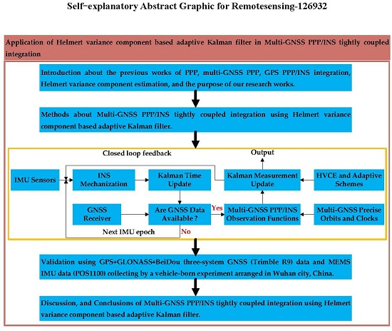
Application of Helmert Variance Component Based Adaptive Kalman Filter in Multi-GNSS PPP/INS Tightly Coupled Integration

Abstract

The integration of the Global Positioning System (GPS) and the Inertial Navigation System (INS) based on Real-time Kinematic (RTK) and Single Point Positioning (SPP) technology have been applied as a powerful approach in kinematic positioning and attitude determination. However, the accuracy of RTK and SPP based GPS/INS integration mode will degrade visibly along with the increasing user-base distance and the quality of pseudo-range. In order to overcome such weaknesses, the tightly coupled integration between GPS Precise Point Positioning (PPP) and INS was proposed recently. 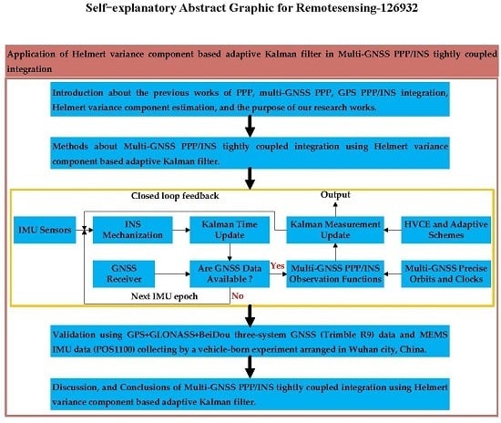Because of the rapid development of the multi-constellation Global Navigation Satellite System (multi-GNSS), we introduce the multi-GNSS into the tightly coupled integration of PPP and INS in this paper. Meanwhile, in order to weaken the impacts of the GNSS observations with low quality and the inaccurate state model on the performance of the multi-GNSS PPP/INS tightly coupled integration, the Helmert variance component estimation based adaptive Kalman filter is employed in the algorithm implementation. Finally, a set of vehicle-borne GPS + BeiDou + GLONASS and Micro-Electro-Mechanical-Systems (MEMS) INS data is analyzed to evaluate the performance of such algorithm. The statistics indicate that the performance of the multi-GNSS PPP/INS tightly coupled integration can be enhanced significantly in terms of both position accuracy and convergence time.

1. Introduction

Since the integration of the Global Positioning System (GPS) and the Inertial Navigation System (INS) was proposed by Cox in 1978 [1], it has been used widely as an effective and precise tool to obtain precise position, velocity, and attitude in many dynamic domains [2,3,4]. Especially, the GPS Single Point Positioning (SPP) [5] based- and Real-time Kinematic (RTK) [6,7] based-GPS/INS integration modes are applied successively because of the easy implementation of SPP and the high accuracy of RTK [8,9,10,11] in recent decades. However, the SPP based integration system can only provide meter level position accuracy [10,11], which can only be used in the regions without high accuracy requirement. Although centimeter level position accuracy can be obtained by using RTK based integration, its performance is highly influenced by the distance between users and base station owing to the decreasing relationship of GPS observations for the station-pair [5]. For most of users, however, a system that can not only provide high accuracy location information, but also overcome the disadvantages in RTK- and SPP- based integration system is urgently required, such as in mobile mapping system and unmanned control system.

Prosperously, the rapid development of GPS Precise Point Positioning (PPP) technology [12] and the ameliorating of satellite precise products [13] make such requirement possible. By adopting the dual-frequency GPS pseudo-range and carrier-phase observations from a single receiver and the satellite precise orbits and clocks provided by International Global Navigation Satellite System (GNSS) Service (IGS), PPP can provide users centimeter position accuracy [12,13,14]. Due to such characters, PPP has been used in some precise applications such as in displacement monitoring and kinematic location determination [14,15,16]. In recent years, some researchers have focused on the integration of GPS PPP and INS for the further performance improvement of PPP. According to previous studies, the GPS PPP/INS tightly coupled integration can not only conquer the insufficiency of RTK- and SPP- based integrations but also improve PPP’s performance in terms of the positioning accuracy and aid GPS carrier-phase cycle slip detection [17,18,19].

However, as is well known, the performance of the PPP/INS tightly coupled integration is determined visibly by that of PPP, especially in the challenging environments. Generally, the PPP accuracy is mainly influenced by the available satellite numbers, the spatial geometry structure between the station and satellites [20], and the quality of pseudo-range observations and the carrier-phase continuity [21]. Usually, the observation quality and continuity have strong relationship with users’ observing condition and it is also hard to control. Therefore, many works were done by focusing on the improvement of the spatial geometry structure in recent years [22]. Thanks to the rapid development of the multi-constellation GNSS in recent years [23], the combination of the multi-GNSS data is considered as a valid and direct way to improve significantly the accuracy of PPP [24,25,26]. According to the studies of Jokinen et al. (2013) and Cai et al. (2013), much better positioning accuracy can be obtained by using GPS and GLONASS data together in PPP calculation compared to that of using GPS only [24,25]. Besides, the study of Li et al. (2015) shows that the feasible performance improvement in terms of position accuracy, availability, continuity, and convergence time of PPP can be obtained by using the combination of GPS, GLONASS, BeiDou, and Galileo [26].

In order to further improve the performance of the GPS PPP/INS tightly coupled integration, the multi-GNSS PPP/INS tightly coupled integration is employed and implemented in a unique Kalman filter in this paper. Due to the reliable estimation accuracy of the Kalman filter [27] is impacted by the accuracy of state model and the accuracy of observation’ a priori covariance [28,29,30,31], the Helmert variance component estimation based adaptive Kalman filter [31,32,33] is applied in our study to weaken the inappropriate the a priori covariance of observations and compensate the impact of the inaccurate state model which can make the multi-GNSS PPP/INS integration solutions more robust. Then, a set of vehicle-borne GPS, BeiDou, GLONASS, and INS data is processed and analyzed to assess the performance of the multi-GNSS PPP/INS tightly coupled integration based on the adaptive Kalman filter with Helmert variance component estimation.

2. Methods

In order to make the algorithm clear, the Kalman filter based multi-GNSS PPP/INS tightly coupled integration model is introduced in detail at first. Then, the multi-GNSS PPP/INS tightly coupled integration based on the adaptive Kalman filter of the Helmert variance component estimation will be described particularly.

2.1. Multi-GNSS PPP/INS Tightly Coupled Integration Functions

As is well known, the Kalman filter has been widely used as an optimal estimator for state parameter calculation in both GNSS and GNSS/INS integration system [28,29,30]. In this research, the closed loop Kalman filter will be adopted to combine the multi-GNSS raw observations and INS navigation results. Briefly, the observation function model for Kalman filter can be given by following equation

$${\mathit{L}}_k={\mathit{H}}_k{\mathit{X}}_k+{\mathit{Z}}_k+{\mathit{\eta }}_k$$

(1)

and the relative linear dynamic model of state parameters (${\mathit{X}}_k$) can be given by following equation

$${\mathit{X}}_k={\mathit{\Phi }}_{k,k-1}{\mathit{X}}_{k-1}+{\mathit{ϵ}}_k$$

(2)

with

$$\begin{array}{c}E\left({\mathit{\eta }}_k\right)=0, Cov\left({\mathit{\eta }}_k,{\mathit{\eta }}_k\right)={\mathit{R}}_{Z,k}\\ E\left({\mathit{ϵ}}_k\right)=0, Cov\left({\mathit{ϵ}}_k,{\mathit{ϵ}}_k\right)={\mathit{Q}}_{X,k} ,Cov\left({\mathit{\eta }}_k,{\mathit{ϵ}}_k\right)=0\end{array}$$

(3)

where ${\mathit{Z}}_k$ is the innovation vector at epoch k computed by making differences between the observed GNSS and the predicted GNSS values computed by using the satellites information and INS updated receiver information; ${\mathit{H}}_k$ and ${\mathit{\Phi }}_{k,k-1}$denote the state parameters’ designed matrix at epoch k and the state transfer matrix from epoch k − 1 to epoch k, respectively; ${\mathit{\eta }}_k$ and ${\mathit{ϵ}}_k$ represent the observation noise with the a priori covariance ${\mathit{R}}_{Z,k}$ and the process noise with the a priori covariance ${\mathit{Q}}_{X,k}$, and both of them are considered to be Gaussian normal distribution; $Cov( )$ is the covariance function.

For the ionospheric-free combination based GPS + BeiDou + GLONASS PPP/INS tightly coupled integration, the innovation function consists of three parts as expressed as

$${\mathit{Z}}_k=\left[\begin{array}{c}{\mathit{Z}}_G\\ {\mathit{Z}}_B\\ {\mathit{Z}}_R\end{array}\right]=\left[\begin{array}{c}{\mathit{L}}_G\\ {\mathit{L}}_B\\ {\mathit{L}}_R\end{array}\right]-\left[\begin{array}{c}{\overline{\mathit{L}}}_G\\ {\overline{\mathit{L}}}_B\\ {\overline{\mathit{L}}}_R\end{array}\right]$$

(4)

with the a priori covariance

$${\mathit{R}}_{Z,k}={\sigma }_0^2{\mathit{P}}_Z^{-1}=\left[\begin{array}{ccc}{\sigma }_G^2{\mathit{P}}_{Z,G}^{-1}& 0& 0\\ 0& {\sigma }_B^2{\mathit{P}}_{Z,B}^{-1}& 0\\ 0& 0& {\sigma }_R^2{\mathit{P}}_{Z,R}^{-1}\end{array}\right]$$

(5)

where the subscript G, B, R denote GPS, BeiDou, and GLONASS, respectively; ${\sigma }^2$ and ${\mathit{P}}_Z$ are variance of unit weight and weight matrix, assuming that the values of ${\sigma }_0^2, {\sigma }_G^2, {\sigma }_B^2$, and ${\sigma }_R^2$ are the same and all of the observations are independent; ${\mathit{R}}_{Z,k}$ denotes the a priori variance matrix of innovation ${\mathit{Z}}_k$; ${\mathit{L}}_k$ and ${\overline{\mathit{L}}}_k$ represent the observed- and the predicted- data of k GNSS system (k = G, B, R), and each of them contains three types observations, namely pseudo-range (P) and carrier-phase ($\phi$) of ionospheric-free combination and Doppler (D), and generally the corresponding a priori variance values are 0.3 m, 0.003 m, and 0.1 m/s. Succinctly, the predicted ${\overline{L}}_G$, ${\overline{L}}_B$, and ${\overline{L}}_R$ can be written as

$${\overline{\mathit{L}}}_G=\left[\begin{array}{c}{\overline{\mathit{L}}}_{G,P}\\ {\overline{\mathit{L}}}_{G,\phi }\\ {\overline{\mathit{L}}}_{G,D}\end{array}\right]=\left[\begin{array}{c}\left|\left|{\mathit{p}}_r-{\mathit{p}}^G\right|\right|+\Delta {\mathit{\rho }}_{G,P}+{\mathit{\ell }}_p\\ \left|\left|{\mathit{p}}_r-{\mathit{p}}^G\right|\right|+\Delta {\mathit{\rho }}_{G,\phi }+{\mathit{\ell }}_p\\ \left|\left|{\mathit{v}}_r-{\mathit{v}}^G\right|\right|+\Delta {\mathit{\rho }}_{G,D}+{\mathit{\ell }}_v\end{array}\right]$$

(6)

$${\overline{\mathit{L}}}_B=\left[\begin{array}{c}{\overline{\mathit{L}}}_{B,P}\\ {\overline{\mathit{L}}}_{B,\phi }\\ {\overline{\mathit{L}}}_{B,D}\end{array}\right]=\left[\begin{array}{c}\left|\left|{\mathit{p}}_r-{\mathit{p}}^B\right|\right|+\Delta {\mathit{\rho }}_{B,P}+{\mathit{\ell }}_p\\ \left|\left|{\mathit{p}}_r-{\mathit{p}}^B\right|\right|+\Delta {\mathit{\rho }}_{B,\phi }+{\mathit{\ell }}_p\\ \left|\left|{\mathit{v}}_r-{\mathit{v}}^B\right|\right|+\Delta {\mathit{\rho }}_{B,D}+{\mathit{\ell }}_v\end{array}\right]$$

(7)

$${\overline{\mathit{L}}}_R=\left[\begin{array}{c}{\overline{\mathit{L}}}_{R,P}\\ {\overline{\mathit{L}}}_{R,\phi }\\ {\overline{\mathit{L}}}_{R,D}\end{array}\right]=\left[\begin{array}{c}\left|\left|{\mathit{p}}_r-{\mathit{p}}^R\right|\right|+\Delta {\mathit{\rho }}_{R,P}+{\mathit{\ell }}_p\\ \left|\left|{\mathit{p}}_r-{\mathit{p}}^R\right|\right|+\Delta {\mathit{\rho }}_{R,\phi }+{\mathit{\ell }}_p\\ \left|\left|{\mathit{v}}_r-{\mathit{v}}^R\right|\right|+\Delta {\mathit{\rho }}_{R,D}+{\mathit{\ell }}_v\end{array}\right]$$

(8)

where $\left|\left|( )\right|\right|$ denotes the Euclidean norm; ${\mathit{p}}_r$ and ${\mathit{p}}^k$ represent receiver (r) position and satellite (k = G, B, R) position; ${\mathit{v}}_r$ and ${\mathit{v}}^k$ are receiver velocity and satellite velocity; $\Delta {\mathit{\rho }}_P$, $\Delta {\mathit{\rho }}_{\phi }$, and $\Delta {\mathit{\rho }}_D$ denote the error corrections for pseudo-range, carrier-phase, and Doppler, respectively [12,13,14]; ${\mathit{\ell }}_p$ and ${\mathit{\ell }}_v$ are the lever-arm corrections [34] of receiver position and receiver velocity, which are caused by the inconsistent reference points of the GNSS receiver and Inertial Measurement Unit (IMU), expresses as

$$\left[\begin{array}{c}{\mathit{\ell }}_p\\ {\mathit{\ell }}_v\end{array}\right]=\left[\begin{array}{c}{\mathit{C}}_n^e{\mathit{C}}_b^n{\mathit{\iota }}^b\\ -{\mathit{C}}_n^e(\left({\mathit{\omega }}_{in}^n\times \right){\mathit{C}}_b^n{\mathit{\iota }}^b-{\mathit{C}}_b^n({\mathit{\iota }}^b\times ){\mathit{\omega }}_{ib}^b)\end{array}\right]$$

(9)

where ${\mathit{C}}_b^n$ is the transfer matrix to transform lever-arm values (${\mathit{\iota }}^b$) in body frame (b-frame, Forward-Right-Down) to navigation frame (n-frame, North-East-Down); ${\mathit{C}}_n^e$ is used to transfer the solutions from n-frame to Earth Centered Earth Fixed Frame (e-frame, World Geodesic System-84); ${\mathit{\omega }}_{in}^n$ and ${\mathit{\omega }}_{ib}^b$ denote the rotation angular rate of n-frame and the angular rate output from gyroscope with respect to inertial frame (i-frame) projected in n-frame; ‘$\times$’ represents the cross-product operation.

Finally, the innovation vector of GPS + BeiDou + GLONASS can be obtained according to the Equations (6)–(9). Meanwhile, the designed matrix ${\mathit{X}}_k$ and state parameters ${\mathit{H}}_k$ can be obtained by the derivation operation of Equations (4), (6)–(8), and the concrete forms can be described as

$${\mathit{X}}_k={\left[\delta \mathit{p} \delta \mathit{v} \delta \mathit{\theta } \delta {\mathit{B}}_g \delta {\mathit{B}}_a\delta {\mathit{S}}_g \delta {\mathit{S}}_a \delta {\mathit{t}}_r \delta T_w \delta {\mathit{N}}_{IF}\right]}^T$$

(10)

$${\mathit{H}}_G=\left[\begin{array}{ccc}\begin{array}{ccc}{\mathit{H}}_{P,p}^G& 0& {\mathit{H}}_{P,\theta }^G\\ {\mathit{H}}_{\phi ,p}^G& 0& {\mathit{H}}_{\phi ,\theta }^G\\ {\mathit{H}}_{D,p}^G& {\mathit{H}}_{D,v}^G& {\mathit{H}}_{D,\theta }^G\end{array}& \begin{array}{ccc}0& 0& {\mathit{H}}_{P,t}^G\\ 0& 0& {\mathit{H}}_{\phi ,t}^G\\ {\mathit{H}}_{D,g}^G& 0& {\mathit{H}}_{D,t}^G\end{array}& \begin{array}{cc}{\mathit{H}}_{P,T}^G& 0\\ {\mathit{H}}_{\phi ,T}^G& {\mathit{H}}_{\phi ,N}^G\\ 0& 0\end{array}\end{array}\right]$$

(11)

$${\mathit{H}}_B=\left[\begin{array}{ccc}\begin{array}{ccc}{\mathit{H}}_{P,p}^B& 0& {\mathit{H}}_{P,\theta }^B\\ {\mathit{H}}_{\phi ,p}^B& 0& {\mathit{H}}_{\phi ,\theta }^B\\ {\mathit{H}}_{D,p}^B& {\mathit{H}}_{D,v}^B& {\mathit{H}}_{D,\theta }^B\end{array}& \begin{array}{ccc}0& 0& {\mathit{H}}_{P,t}^B\\ 0& 0& {\mathit{H}}_{\phi ,t}^B\\ {\mathit{H}}_{D,g}^B& 0& {\mathit{H}}_{D,t}^B\end{array}& \begin{array}{cc}{\mathit{H}}_{P,T}^B& 0\\ {\mathit{H}}_{\phi ,T}^B& {\mathit{H}}_{\phi ,N}^B\\ 0& 0\end{array}\end{array}\right]$$

(12)

$${\mathit{H}}_R=\left[\begin{array}{ccc}\begin{array}{ccc}{\mathit{H}}_{P,p}^R& 0& {\mathit{H}}_{P,\theta }^R\\ {\mathit{H}}_{\phi ,p}^R& 0& {\mathit{H}}_{\phi ,\theta }^R\\ {\mathit{H}}_{D,p}^R& {\mathit{H}}_{D,v}^R& {\mathit{H}}_{D,\theta }^R\end{array}& \begin{array}{ccc}0& 0& {\mathit{H}}_{P,t}^R\\ 0& 0& {\mathit{H}}_{\phi ,t}^R\\ {\mathit{H}}_{D,g}^R& 0& {\mathit{H}}_{D,t}^R\end{array}& \begin{array}{cc}{\mathit{H}}_{P,T}^R& 0\\ {\mathit{H}}_{\phi ,T}^R& {\mathit{H}}_{\phi ,N}^R\\ 0& 0\end{array}\end{array}\right]$$

(13)

where the symbol $\delta$ denotes error; $\mathit{p}$, $\mathit{v}$, and $\mathit{\theta }$ represent position, velocity, and attitude, respectively; B and S are the biases vector and scale factors vector of gyroscopes (g) and accelerometers (a); ${\mathit{t}}_r=\left[t t_{B-G} t_{R-G} \dot{t}\right]$ is receiver clock related parameter vector, here $t$ and $\dot{t}$ are basic receiver clock offset and clock drift, $t_{B-G}$ and $t_{R-G}$ are the Inter-System Biases (ISB) of BeiDou and GLONASS with respect to basic clock (GPS), and such ISBs are caused by the different signal structure and the different hardware delay of each individual GNSS system in a same receiver and they are rather stable [26]; $T_w$ is the wet component of the tropospheric zenith delay and ${\mathit{N}}_{IF}$ is the ionospheric-free combination ambiguity vector; ${\mathit{H}}_{m,l}^k$ represents the derived coefficient matrix of l parameter (l = $\mathit{p}$, $\mathit{v}$, $\mathit{\theta }$…) for m (m = P, $\phi$, D) observations in k (k = G, B, R) GNSS system.

Usually, the constant velocity (CV) model and constant accelerometer (CA) model are adopted to describe the behavior of the position and velocity in the GNSS calculations [35]. For the GNSS/INS integration system, another precise dynamic model is adopted to describe the behavior of the position, velocity, and attitude with the expression [8,9]

$$\left[\begin{array}{c}\delta {\dot{\mathit{p}}}^n\\ \delta {\dot{\mathit{v}}}^n\\ \delta \dot{\mathit{\theta }}\end{array}\right]=\left[\begin{array}{c}-{\mathit{\omega }}_{en}^n\times \delta {\mathit{p}}^n+\delta {\mathit{v}}^n\\ -\left({\mathit{\omega }}_{in}^n+{\mathit{\omega }}_{ie}^n\right)\times \delta {\mathit{v}}^n+{\mathit{f}}^n\times \mathit{\theta }+\delta {\mathit{g}}^n+{\mathit{C}}_b^n\delta {\mathit{f}}^b\\ -{\mathit{\omega }}_{in}^n\times \mathit{\theta }-{\mathit{C}}_b^n\delta {\mathit{\omega }}_{ib}^b\end{array}\right]$$

(14)

where ${\mathit{\omega }}_{en}^n$ and ${\mathit{\omega }}_{ie}^n$ denote the rotation angular rate of n-frame with respect to e-frame projected in n-frame and the rotation angular rate of e-frame with respect to inertial frame (i-frame) projected in n-frame; ${\mathit{f}}^b$ and ${\mathit{g}}^n$ are specific forces projected in b-frame from accelerometers and gravity vector projected in n-frame.

To enhance the INS performance during the GNSS outage periods visibly, the scale factors and biases are also estimated along with other parameters [36] in the GNSS/INS tightly coupled integration system. Generally, such errors in IMU data can be expressed as a constant part and a random part [37,38]. The constant part can be compensated in the hardware calibration stage ordinarily, but the random part cannot be calibrated accurately. Thus, it is usually modeled as the first order Gauss-Markov procedure [27] and estimated by Kalman filter, and their discrete time models are described by

$$\delta {\mathit{B}}_k=e^{-\Delta t_k/\tau }\delta {\mathit{B}}_{k-1}+w_{B,k-1}$$

(15)

$$\delta {\mathit{S}}_k=e^{-\Delta t_k/\tau }\delta {\mathit{S}}_{k-1}+w_{S,k-1}$$

(16)

where $\Delta t_k$ and $\tau$ are interval of two adjacent IMU epochs and the correlation time determined by IMU hardware accuracy level; $w$ is the white driving noise with zero expectation and variance value $2{\sigma }^2\Delta t/\tau$, here $\sigma$ is the statistics square mean values of IMU hardware. In this paper, the $\sigma$ values of the gyroscope biases and scale factors are 0.5 °/$h$ and 150 ppm/$\sqrt{h}$, and these of the accelerometer biases and scale factors are 0.3 m/$s^2$ and 150 ppm/$\sqrt{h}$.

Besides, some classic stochastic models as described in [27] are adopted to describe the behaviors of the receiver clock offset and drift, the residual of the wet component of the tropospheric zenith delay and the inter-system biases, and the ambiguity, which can be generally written as

$$\delta t_k=\delta t_{k-1}+\delta {\dot{t}}_{k-1}+{\upsilon }_{t,k-1}$$

(17)

$$\delta {\dot{t}}_k=\delta {\dot{t}}_{k-1}+{\upsilon }_{\dot{t},k-1}$$

(18)

$$\delta IS{B}_k=\delta IS{B}_{k-1}+{\upsilon }_{ISB,k-1}$$

(19)

$$\delta T_{w,k}=\delta T_{w,k-1}+{\upsilon }_{T_{w,k-1}}$$

(20)

$$\delta N_{IF,k}=\delta N_{IF,k-1}+{\upsilon }_{N_{IF,k-1}}$$

(21)

where $\upsilon$ is driving noise with different Power Spectral Density (PSD) value. It should be noticed that these PSD are generally nonzero values except the ambiguity’s PSD. The process noise values of Equations (17)–(21) are 0.19 m/$\sqrt{h}$, 0.37 m/s/$\sqrt{h}$, 0.005 m/$\sqrt{h}$, 0.01 m$/\sqrt{h}$ and 0.0 m$/\sqrt{h}$, respectively.

According to the models mentioned above, the time update phase and measurement update phase for the multi-GNSS PPP/INS tightly coupled integration can be finished by following equations

$$\left[\begin{array}{c}{\mathit{X}}_{k.k-1}\\ {\mathit{P}}_{X,k,k-1}\end{array}\right]=\left[\begin{array}{c}{\mathit{\Phi }}_{k,k-1}{\mathit{X}}_{k-1}\\ {\Phi }_{k,k-1}{\mathit{P}}_{X,k-1}{\Phi }_{k,k-1}^T+{\mathit{Q}}_{X,k-1}\end{array}\right]$$

(22)

$$\left[\begin{array}{c}{\mathit{X}}_k\\ {\mathit{P}}_{X,k}\end{array}\right]=\left[\begin{array}{c}{\mathit{X}}_{k,k-1}+{\mathit{K}}_k\left({\mathit{Z}}_k-{\mathit{H}}_k{\mathit{X}}_{k,k-1}\right)\\ (\mathit{I}-{\mathit{K}}_k){\mathit{P}}_{X,k,k-1}{(\mathit{I}-{\mathit{K}}_k)}^T+{\mathit{K}}_k{\mathit{R}}_{Z,k}{\mathit{K}}_k^T\end{array}\right]$$

(23)

$${\mathit{K}}_k={\mathit{P}}_{X,k,k-1}{\mathit{H}}_k^T\left({\mathit{H}}_k{\mathit{P}}_{X,k,k-1}{\mathit{H}}_k^T+{\mathit{R}}_{Z,k}\right)$$

(24)

where ${\mathit{X}}_{k.k-1}$ and ${\mathit{P}}_{X,k,k-1}$denote the predicted state parameter vector and the corresponding variance; ${\mathit{P}}_X$ is the variance of state parameter vector; ${\mathit{K}}_k$ and $\mathit{I}$ are the gain matrix and unit matrix.

2.2. Helmert Variance Component Estimation Based Adaptive Kalman Filter

The observation quality of each individual GNSS is not the same due to the different signal structures, frequencies, signal-to-noise ratios, and the signal transmission paths. It means that the a priori variance value is different for each GNSS system, even for each satellite. Fortunately, the variance for individual observations or for different grouped data can be estimated posteriorly by the Helmert variance component estimation (HVCE) [31,32,33] based on the posterior measurement residuals. In this research, we assume the component of each single GNSS system data is the same and the observations are divided into three groups (GPS, BeiDou, and GLONASS) at every epoch. The corresponding residual groups can be obtained from Equations (1), (4), (23) and (24) with the expression of

$${\mathit{V}}_k={\mathit{H}}_k{\mathit{X}}_k-{\mathit{Z}}_k=\left[\begin{array}{c}{\mathit{V}}_G\\ {\mathit{V}}_B\\ {\mathit{V}}_R\end{array}\right]=\left[\begin{array}{c}{\mathit{H}}_G\\ {\mathit{H}}_B\\ {\mathit{H}}_R\end{array}\right]{\mathit{X}}_k-\left[\begin{array}{c}{\mathit{Z}}_G\\ {\mathit{Z}}_B\\ {\mathit{Z}}_R\end{array}\right]$$

(25)

where ${\mathit{V}}_k$ is the multi-GNSS’s posterior residual vector including the GPS residuals (${\mathit{V}}_G$), BeiDou residuals (${\mathit{V}}_B$), and GLONASS residuals (${\mathit{V}}_R$). According to the HVCE theory, the formula for estimating independent measurements’ components can be defined as

$$\left[\begin{array}{c}{\sigma }_G^2\\ {\sigma }_B^2\\ {\sigma }_R^2\end{array}\right]={\left[\begin{array}{c}\begin{array}{ccc}{s}_{G,G}& s_{G,B}& s_{G,R}\end{array}\\ \begin{array}{ccc}{s}_{B,G}& s_{B,B}& s_{B,R}\end{array}\\ \begin{array}{ccc}{s}_{R,G}& s_{R,B}& s_{R,R}\end{array}\end{array}\right]}^{-1}\left[\begin{array}{c}{\mathit{V}}_G^T{\mathit{P}}_{Z,G}{\mathit{V}}_G\\ {\mathit{V}}_B^T{\mathit{P}}_{Z,B}{\mathit{V}}_B\\ {\mathit{V}}_R^T{\mathit{P}}_{Z,R}{\mathit{V}}_R\end{array}\right]$$

(26)

$$\begin{array}{c}{s}_{k,k}=n_k-2tr\left({\mathit{N}}^{-1}{\mathit{N}}_k\right)+tr\left({\mathit{N}}^{-1}{\mathit{N}}_k{\mathit{N}}^{-1}{\mathit{N}}_k\right)\\ s_{k,j}=s_{j,k}=\text{tr}\left({\mathit{N}}^{-1}{\mathit{N}}_k{\mathit{N}}^{-1}{\mathit{N}}_j\right) \\ \mathit{N}={\mathit{H}}^T{\mathit{P}}_Z^{-1}\mathit{H}, k,j=\left(G,B,R\right)\end{array}\}$$

(27)

where ‘tr’ denotes the trace operation for matrix; n is the available GNSS satellite number. The values in right part of Equation (26) can be calculated by Equations (5), (25) and (27). It is clear that the function numbers are the same to the state parameters, which means the variance components can be estimated exclusively. Then the estimated components are utilized to redefine the weight matrix in Equation (5) by

$$\begin{array}{c}{\overline{\mathit{P}}}_{Z,k}=\frac{{\mathit{P}}_{Z,k}{c}_0}{{\sigma }_k^2}, k=G, B,R\\ {\overline{\mathit{R}}}_Z=\left[\begin{array}{ccc}{\sigma }_G^2{\overline{\mathit{P}}}_{Z,G}^{-1}& 0& 0\\ 0& {\sigma }_B^2{\overline{\mathit{P}}}_{Z,B}^{-1}& 0\\ 0& 0& {\sigma }_R^2{\overline{\mathit{P}}}_{Z,R}^{-1}\end{array}\right]\end{array}$$

(28)

where $c_0$ is an arbitrary constant, which is usually selected from one of the estimated variance components (${\sigma }_G^2$ is used in this paper). The redefined weight matrix will be used to calculate the refined covariance matrix ${\overline{\mathit{R}}}_Z$ which will be applied for the state parameter re-estimation (${\overline{\mathit{X}}}_k$) in Equations (23) and (24). Then, an iterative operation from Equations (23) and (24) to Equations (26)–(28) will be worked at each GNSS epoch until the differences among ${\sigma }_G^2$, ${\sigma }_B^2$, and ${\sigma }_R^2$ each other is less than a certain given threshold. Then, the GNSS system providing higher accuracy observations will be entrusted bigger weight and have more effects on the state estimation via the Kalman gain matrix in Equation (24).

Besides the effects of observations, the inaccurate state model can also influence the performance of the PPP/INS integration. Such effect can be detected by the differences between re-estimated state parameter ${\overline{\mathit{X}}}_k$ and that of the predicted value ${\mathit{X}}_{k.k-1}$ with the formulation of

$$\Delta {\tilde{\mathit{X}}}_k=\left|{\overline{\mathit{X}}}_k-{\mathit{X}}_{k.k-1}\right|/\sqrt{tr\left({\mathit{P}}_{X,k-1}\right)}$$

(29)

$$\mathit{\alpha }=\{\begin{array}{c}1 \Delta {\tilde{\mathit{X}}}_k\le c_1\\ \begin{array}{c}\frac{\Delta {\tilde{\mathit{X}}}_k}{c_1}{\left(\frac{c_2-c_1}{c_2-\Delta {\tilde{\mathit{X}}}_k}\right)}^2 c_1<\Delta {\tilde{\mathit{X}}}_k\le c_2\\ \infty \Delta {\tilde{\mathit{X}}}_k>c_2\end{array}\end{array}$$

(30)

where $\mathit{\alpha }$ is the adaptive factor; $c_1=1.0~1.5$ and $c_2=3.0~4.5$ are the threshold constants [31].

From Equations (26)–(30), the final form of the gain matrix can be written as

$${\overline{\mathit{K}}}_k=\mathit{\alpha }{\mathit{P}}_{X,k,k-1}{\mathit{H}}_k^T\left({\mathit{H}}_k\mathit{\alpha }{\mathit{P}}_{X,k,k-1}{\mathit{H}}_k^T+{\overline{\mathit{R}}}_{Z,k}\right)$$

(31)

and the corresponding measurement update phase of HVCE based adaptive Kalman filter can be redefined as

$$\left[\begin{array}{c}{\overline{\mathit{X}}}_k\\ {\overline{\mathit{P}}}_{X,k}\end{array}\right]=\left[\begin{array}{c}{\mathit{X}}_{k,k-1}+{\overline{\mathit{K}}}_k\left({\mathit{Z}}_k-{\mathit{H}}_k{\mathit{X}}_{k,k-1}\right)\\ (\mathit{I}-{\overline{\mathit{K}}}_k){\mathit{P}}_{X,k,k-1}{(\mathit{I}-{\overline{\mathit{K}}}_k)}^T+{\overline{\mathit{K}}}_k{\overline{\mathit{R}}}_{Z,k}{\overline{\mathit{K}}}_k^T\end{array}\right]$$

(32)

where these symbols are the same as these given in Equation (23). From the above expressions, the HVCE based adaptive Kalman filter will make the multi-GNSS PPP/INS integration solutions more optimal. On one hand, the redefined posteriori ${\overline{\mathit{R}}}_{Z,k}$ will allot bigger weight for better quality GNSS system observations and limit the effect of the lower quality measurements. On the other hand, by using the adaptive factor, the contribution of the current measurements and the previous epochs’ state information can be adjusted.

2.3. Implementation of Multi-GNSS PPP/INS Tightly Coupled Integration

According to the algorithm description above, the implementation of the HVCE based adaptive Kalman filter for the multi-GNSS PPP/INS tightly coupled integration is briefly depicted in Figure 1. Sententiously, when the attitude alignment and initialization of the parameter vector and the corresponding covariance matrix are finished, the INS mechanization, the Kalman time update phase, and the GNSS availability checking functions will work. If the GNSS is unavailable, the whole system will return to next IMU epoch for INS data processing. Otherwise, the Kalman measurement update phase (including the HVCE and adaptive factor operation) will be activated. Then, the estimated parameters will be output and feedback by a closed loop to compensate the IMU data hardware errors.

3. Experiment Data

To evaluate the application of the HVCE based adaptive Kalman filter in the multi-GNSS PPP/INS tightly coupled integration, we analyzed a set of GPS, BeiDou, GLONASS, INS data collected by a land vehicle test arranged around Wuhan City in China and equipped with POS1100 (Micro Electro Mechanical Sensor grade IMU, MEMS), POS830 (navigation grade IMU) and Trimble NetR9 (geodetic receiver) multi-GNSS receiver. The POS1100 and POS830 were provided by Wuhan MP Space Time Technology Company (Wuhan, China). The corresponding main performance parameters of such two IMU sensors are shown in

Table 1. Parameters of the IMU sensors used in the data processing.

IMU	Grade	Dimensions (mm)	Weight (kg)	Gyro Bias (°/h)	Angular Random Walk °/$\sqrt{\mathit{h}}$
POS830	Navigation	190 × 191 × 183	9.0	0.005	0.002
POS1100	MEMS	81.8 × 68 × 70	0.5	10.0	0.33

.

3.1. Data Processing Strategies and Models

In the data processing phase, the dual-frequency (GPS: L1/L2; GLONASS: L1/L2; BeiDou: B1/B2) GNSS pseudo-range, carrier-phase, Doppler, and increments of angular and velocity are used. The interval of GNSS observations and IMU data are 1.0 s and 0.005 s respectively. The satellites with elevation angle less than 10° are eliminated. The precise satellite orbit and clock products from GNSS Research Center (GRC), Wuhan University are adopted to weaken the effects of the satellite orbit and clock on the GNSS precise positioning accuracy. Besides, the classical error models of the troposphere delay, ionosphere delay, earth rotation effect, relativity effect, phase center offset (PCO) and variation (PCV) of satellite and receiver, phase wind-up, solid and ocean tide, pole tide, etc. are used for the GNSS observation errors correction [12,13,25,26]. The INS error compensation models such as the coning correction model, the rotational and sculling motion models [8,9] are applied to remove the influences of the axis motion of the IMU sensors on INS velocity and attitude update. In the PPP/INS tightly coupled integration, the position, velocity, and attitude of receiver, the IMU biases and scale factors, the receiver clock and drift, the wet component residual of the zenith tropospheric delay, the inter-system biases and inter-frequency biases, and the ambiguities are estimated as parameters.

3.2. Dynamic Property and Satellites Availability

Figure 2 shows the velocities and attitudes of vehicle platform in the experiment. Accordingly, the average velocities are about 13.4 m/s, 7.2 m/s, and 0.1 m/s in North, East, and Up directions, respectively. From the attitudes results in heading component, it is mainly around 160° and 340°, which means the platform almost moved along the North-West to the South-East direction. When the vehicle turned back to the next route, the heading angle changed frequently (around about 215,000 s, 23,000 s, 25,000 s, and 27,000 s). It is noted that the road is uneven according to the vertical velocity (shown in purple box) and pitch attitude. The trajectory of this test is shown in the subfigure in Figure 3. The distances are about 9.7 km along the East-West direction and about 3.5 km along the North-South direction. The red point shown in the trajectory subfigure of Figure 3 is a GNSS partial outage, and the corresponding available satellites number are depicted in the red dashed box of Figure 4.

The sky plot of the GNSS satellites during the experiment is depicted in Figure 3. As is well known, currently the constellation of GPS and GLONASS consists of Medium Earth Orbit (MEO) satellite only and BeiDou constellation consists of MEO satellites (did not be tracked in this test), Geostationary Earth Orbit (GEO) satellites (B01, B02, B03, and B04 in Figure 2), and Inclined Geo-Synchronous Orbit (IGSO) satellites (B07, B08, and B10 in Figure 2). For this experiment arranged in China, BeiDou system can provide better satellite continuity than both GPS and GLONASS own to its GEOs and IGSOs constellation, which is shown clearly in Figure 4. Meanwhile, it is visible that there are more available satellites in view while using the multi-GNSS observations compared to use GPS only, which can be obtained directly from the availability of GPS (G), BeiDou (B), GLONASS (R) satellites as shown in Figure 4. More satellites will lead to better continuity and availability of satellite and better positioning dilution of precision (PDOP), which can be seen clearly in Figure 5. According to the statistics, the average satellite numbers for GPS, G + R, G + B, and G + R are 8.6, 14.3, 15.0, and 20.7, respectively and the corresponding mean PDOP values are 2.1, 1.5, 1.7, and 1.3.

4. Validation of Multi-GNSSPPP/INS Tightly Coupled Integration

In order to give an evident expression for the method adopted in this paper, the whole data are processed in three modes: the GNSS PPP mode, the Kalman filter based GNSS PPP/INS (POS1100) tightly coupled integration mode, and the HVCE adaptive Kalman filter based mode, respectively. To evaluate their performances, the multi-GNSS based RTK/INS (POS830) loose coupled integration results are used as the reference values. In addition, the differences between the references values and the solutions of such three modes in e-frame are transformed into North-East-Up (N, E, and U) directions. Meanwhile, since the convergence time is needed, all of the first 15-min solutions were neglected in calculating the Root Mean Square (RMS) values.

4.1. Dynamic Position Accuracy of Multi-GNSS PPP and PPP/INS Tightly Coupled Integration

As mentioned in the introduction part, the previous works about the influence of the multi-GNSS on PPP mainly focused on the static mode [24,25,26]. Therefore, it is necessary to have a brief view about the impact of the multi-GNSS on PPP performance in the dynamic mode. The corresponding position offsets time series calculated by single-system (GPS) PPP, two-type-satellite-system (G + R and G + B) PPP, and three-type-satellite-system (G + R + B) PPP are shown in Figure 6. The solutions indicate that the multi-GNSS can enhance the performance of PPP by increasing available satellites number and optimizing the spatial geodetic structure in term of PDOP (as shown in Figure 5), which is very important for the dynamic applications in urban environments. According to the statistics in top-subfigure of Figure 7, the RMSs have been improved from 21.9 cm, 27.7 cm, and 15.2 cm of GPS PPP to 6.2 cm, 7.6 cm, and 6.2 cm of G + R + B PPP with the improving percentages of 71.6%, 72.7%, and 59.3% in North, East, Up components, respectively. When adopt G + R or G + B data, similar conclusions can also be obtained by comparing GPS PPP solutions and the average improvement for position are about 37.0%, 45.2%, and 34.0% (Shown in

Table 2. Position improvement percentages of the PPP mode, the PPP/INS tightly coupled integration mode without and with the HVCE and adaptive schemes using G + R, G + B, and G + R + B data by comparing with the corresponding GPS based solutions.

Items	PPP			PPP/INS			HVCE Adaptive PPP/INS
	North	East	Up	North	East	Up	North	East	Up
G + R (%)	24.8	35.8	45.1	24.2	30.3	57.5	39.6	49.6	69.5
G + B (%)	49.1	54.6	23.0	46.9	45.1	58.9	51.4	59.5	68.8
G + R + B (%)	71.6	72.7	59.3	60.4	53.7	68.7	64.3	58.7	70.6

). Besides the RMS, the continuity of PPP can be also ameliorated appreciably. It is very useful, especially in the challenging environments (users’ observing condition leading to the satellite signals loss as the red dashed box shown in Figure 4).

Then, the experiment data were computed in the PPP/INS tightly coupled integration mode by using GPS, G + R, G + B, and G + R + B data, respectively without HVCE adaptive schemes being applied. The corresponding time series of position offsets compared to the references values are depicted in Figure 8 and the RMS values are shown in middle subfigure of Figure 7. Significantly, comparing the results as shown in Figure 8 with these as shown in Figure 6, we can see that the position accuracy of PPP is improved visibly with the aids of the INS information. The average position ameliorating percentages are about 21.2%, 27.7%, and 16.5% in North, East, Up directions, respectively, except that about 1.3 cm position accuracy is lost in vertical when use GPS data. However, as shown in

Table 3. Improvements of the GNSS PPP/INS tightly coupled integration using GPS, G + R, G + B, and G + R + B data by comparing with the corresponding PPP solutions.

Items	GPS	G + R	G + B	G + R + B
North	+6.4 cm/+29.1%	+4.7 cm/+28.5%	+2.9 cm/+26.1%	+0.1 cm/+0.9%
East	+11.6 cm/+42.0%	+6.6 cm/+37.0%	+3.8 cm/+29.9%	+0.1 cm/+1.9%
Up	−1.3 cm/−8.5%	+1.3 cm/+15.9%	+4.9 cm/+42.1%	+1.0 cm/+16.5%

, such improvements seems to decrease from about 10 cm to less than 1 cm along with the increasing the GNSS systems. It may be caused by the fact that the absolute position accuracy of the GNSS/INS integration depends heavily on the accuracy of GNSS. Hence, when three-type-satellite-system (G + R + B) GNSS data are adopted together, the G + R + B PPP can provide good enough position accuracy. In this case, even the INS information is utilized in G + R + B PPP calculations, the effectiveness would also be inconspicuous. Besides the improvements in continuity and accuracy, the enhancing in position stability is also remarkable. The main cause could be the strong constraint for the two adjacent epochs, which is due to the high interdependency of the INS information in short-term period. Besides, compared to the GPS based solutions, when use the multi-GNSS data (G + R, G + B, and G + R + B) the average improvement percentages are about 43.8%, 43.0%, and 61.7% in the three position components (shown in Table 2).

4.2. Position Aaccuracy of Multi-GNSS PPP/INS Tightly Coupled Integration Using HVCE Based Adaptive Kalman Filter

As mentioned in the ”Methods” part, the observation quality for each individual GNSS system maybe not exactly the same. Thus, there could be accuracy loss in the multi-GNSS PPP and/or the multi-GNSS PPP/INS tightly coupled integration if there were no suitable methods for applications to make the observation quality of each individual GNSS system to match the real situation as close as possible. Shown in Figure 9 are the position offsets of the PPP/INS tightly coupled integration of the Helmert variance component estimation based adaptive Kalman filter, and the corresponding statistics are listed in bottom subfigure of Figure 7. Accordingly, the improvements mainly appear as stability and accuracy. According to the results listed in

Table 4. Improvements of the GNSS PPP/INS tightly coupled integration with the aids of the Helmert variance component estimation based adaptive Kalman filter by using GPS, G + R, G + B, and G + R + B data.

Items	GPS	G + R	G + B	G + R + B
North	+0.0 cm/+0.1%	+2.4 cm/+20.4%	+0.7 cm/+8.6%	+0.6 cm/+10.0%
East	−0.6 cm/−3.9%	+2.8 cm/+24.8%	+2.1 cm/+23.3%	+0.5 cm/+ 7.2%
Up	+1.4 cm/+8.4%	+2.4 cm/+34.3%	+2.1 cm/+30.5%	+0.7 cm/+16.5%

, the maximum increase percentages are 20.4%, 24.8%, and 34.3% in North, East, and Up directions, respectively, and the average improvement percentage values are 9.8%, 12.9%, and 21.8%. The position RMS of the HVEC based adaptive Kalman filter G + R + B PPP/INS tightly coupled integration solutions are 5.6 cm, 6.9 cm, and 4.5 cm with the improvements of 10.0%, 7.2%, and 13.9% compared to the corresponding ones of the Kalman filter based G + R + B PPP/INS integration. It means that when the HVEC based adaptive scheme is applied to the multi-GNSS data process, appreciable improvements will be obtained. In addition, as listed in Table 2, the solutions of the multi-GNSS is better than these solutions of GPS only. Meanwhile, by comparing the two-type-satellite-system position solutions in Figure 6, Figure 8 and Figure 9, it is visible that the results calculated by GPS and BeiDou data are a little better than those by GPS+GLONASS data.

4.3. Performance of Velocities and Attitudes

Besides the positions, the PPP/INS integration can also provide users high accuracy velocity and attitude solutions. As plotted in Figure 10, the average RMSs of PPP velocity are 4.3 cm/s, 3.2 cm/s, and 4.4 cm/s in three directions, and the differences of velocity solutions calculated by the single- and the multi-GNSS data in PPP mode are less than 0.7 cm/s. Similarly, the results differences of the PPP/INS tightly coupled integration using different GNSS data are less than 0.3 cm/s, except that the velocity accuracy is enhanced to better than 1.1 cm/s, 1.1 cm/s, and 1.6 cm/s in North-East-Up components, respectively. In addition, visibly, there are little improvements (less than 0.1 cm/s) in velocity when using the HVCE based adaptive Kalman filter in the multi-GNSS PPP/INS tightly coupled integration mode. For attitude solutions, similar conclusions can also be obtained from the statistics as shown by Figure 11. The average RMS of attitudes are about 0.139°, 0.099°, and 0.675° in roll, pitch, and heading components with the differences no more than 0.009°, 0.001°, and 0.017°. It means that the enhancing values in velocity and attitude are limited no matter using the single- or the multi-GNSS data in the PPP/INS tightly coupled integration mode with or without the HVCE based adaptive scheme.

4.4. Multi-GNSS Observation Quality and Residuals

Generally, in the multi-GNSS data processing phase, the a priori variances of pseudo-range and carrier-phase for each GNSS system are treated as the same (for example, 0.3 m for pseudo-range and 0.003 m for carrier-phase). Then, the elevation angle dependent formulation is applied to distinguish the impacts of each satellite on the GNSS solutions. However, it will not be true because of the different special signal structures adopted by different GNSS systems. By selecting the variance component of GPS as an arbitrary constant in Equation (26), we obtained the weight of GPS, BeiDou, and GLONASS by making quotients operation between the variance components of BeDou plus GLONASS and these of GPS. Such variance values are estimated by the Helmert variance component estimation in the PPP/INS tightly coupled integration mode by using G + R + B, G + R, and G + B observations. According to the results as depicted in Figure 12, the influences of the three-type-satellite-system or two-type-satellite-system on positioning change with time. These changings perform similar trend along with the time-varying of the available GPS satellite numbers and PDOP (Figure 5). Besides, it seems BeiDou system is allotted bigger weight than GLONASS in the data processing. It may be one of the facts that the solutions calculated using GPS + BeiDou data is a little better than that of using GPS+GLONASS data. In addition, the weight of BeiDou (or GLONASS) computed by three type-satellite-system (G + R + B) is not completely consistent with these obtained from two type-satellite-system (G + R or G + B, the red (green) line and the pink (deep green) line shown in Figure 12). Meanwhile, bigger weight means the GNSS system provides better quality observations, and theoretically, it is reflected by the observation residuals. Shown in Figure 13 are the observation residuals of each available GPS, BeiDou, and GLONASS satellites of this experiment. Visibly, the average values of pseudo-range and carrier-phase of BeiDou are 87 cm and 0.7 cm, which are smaller than those of GPS (96 cm, 1.0 cm) or GLONASS (148 cm and 1.1 cm). In addition, the qualities of BeiDou GEO satellites (PRN = 36~39, in Figure 13) are worse than those of IGSO satellites (PRN = 42~45). It may be due to the lower accuracy of the BeiDou GEO orbit and clock products.

4.5. Impacts of HVCE Based Adaptive Algorithm on The Convergence Performance of Multi-GNSS PPP/INS Tightly Coupled Integration

As is well known, the limitation of the GPS PPP application in dynamic domains is that it needs a long time for carrier-phase ambiguities to converge to their real values, which controls the high accuracy position of PPP. In addition, such convergence time of PPP can be accessed in term of position accuracy. According to a previous study [36], the convergence time of GPS PPP can be shortened visibly with the help of INS. Based on this work, we will further evaluate the impacts of the HVCE based adaptive scheme on the convergence of the multi-GNSS PPP/INS tightly coupled integration.

The whole data were simulated into nine GNSS outage periods every 15 min with the outage time setting to 10 s. The simulation data were re-processed in the PPP/INS tightly coupled integration mode with and without the HVCE based adaptive Kalman filter. The corresponding position offsets compared to the references values are depicted in Figure 14 and Figure 15. The position spikes as shown in these two figures are caused mainly by the position drift character of INS and the bad initial position accuracy of the PPP/INS tightly coupled integration. Firstly, only IMU data can be adopted to update the position during the GNSS outage periods, and the IMU sensor errors will make the INS updated positions drift along with the GNSS outage time. After each GNSS outage, uncertain time is obligatory for either the PPP mode or the PPP/INS tightly coupled integration mode to converge the GNSS ambiguities gradually. Usually, the INS position drifts during the GNSS outage periods are random and cannot be improved but using the higher grade IMU sensors. However, the bad initial position accuracy of PPP can be ameliorated by using the multi-GNSS data, INS, adaptive algorithm, etc. Significantly, the initialization performance of the PPP/INS tightly coupled integration is improved visibly in terms of initial position accuracy and convergence time by applying the HVCE based adaptive scheme. It may be due to the fact that the HVCE algorithm can provide more reasonable weights for both good quality observations and low quality observations so that the good quality data will play more important roles in PPP/INS computation and the effect of the low quality values will be constrained. Meanwhile, according to the study in reference [21], there is strong relationship between the observation quality and the PPP convergence time. Therefore, it will accelerate the convergence and re-convergence time of the PPP/INS tightly coupled integration by distinguishing the good quality observations from the whole observations. According to the statistics as shown by Figure 14 and Figure 15, the HVCE adaptive based PPP/INS tightly coupled integration can provide the best initial position accuracy with the values of 11.6 cm, 14.3 cm, and 14.0 cm in North, East, and Up components, respectively. In general, the improvements in north and vertical components are more obvious than that in east direction, and the maximum improvements in all of the three directions are about 40.0%, 7.6%, and 27.0%.

5. Discussion

Based on the previous researches of the multi-GNSS PPP [24,25,26], the GPS PPP/INS tightly coupled integration [17,18,19,36], and the Helmert variance component estimation based adaptive Kalman filter [31,33], we did the research on the fusion of these algorithms together. According to our results, it is clear that the position accuracy can be improved visibly by using the multi-GNSS data in both PPP only mode and the PPP/INS tightly coupled integration mode with and without the HVCE based adaptive aiding compared to the GPS-only based solutions. Generally, the average improvements in PPP mode are statistically about 48.5%, 54.3%, and 42.4% in North, East, and Up directions (Table 2), respectively. Similar conclusions can also be obtained in the research of Li et al. (2015) [26]. Compared to GPS based results, there are about 43.8%, 43.0%, and 61.7% improvements in the multi-GNSS PPP/INS integration mode and about 51.8%, 55.9%, and 69.7% improvements in the HVCE based adaptive aid the multi-GNSS PPP/INS integration mode (Table 2).

According the researches from Roesler and Martell (2009), Du (2010), Gao et al. (2015), INS can enhance the performance of GPS PPP [18,19,36]. From our results shown in Table 3, the average position improvements of the single-and the multi-GNSS PPP obtained by the INS augmentation are about 21.2%, 27.7%, and 16.5% in three components. Furthermore, such average improvements will increase to about 28.9%, 36.9%, and 33.3% while adopting the HVCE based adaptive Kalman filter. Besides, about 9.8%, 12.9%, and 21.8% position enhancements in North, East, and vertical directions can be achieved by comparing the solutions of the PPP/INS tightly coupled integration mode without and with the HVCE based adaptive algorithm. Finally, we can obtain about 74.7%, 75.1%, and 70.8% position improvements in North, East, and vertical components by applying the multi-GNSS, the INS, and the Helmert variance component estimation based adaptive Kalman filter to GPS PPP together. Meanwhile, according to the GNSS outage simulations results, the convergence performance can also be improved by using the HVCE based adaptive Kalman filter in the PPP/INS tightly coupled integration. However, these methods have little impacts on the accuracy enhancing of velocimetry and attitude determination of the GPS PPP/INS tightly coupled integration.

6. Conclusions

In this paper, we applied the Helmert variance component estimation based adaptive Kalman filter to the multi-GNSS PPP/INS tightly coupled integration system. By using such Kalman filter, the problems that the a priori variances of different GNSS systems are not the same and the a priori state model mismatches the real motion can be solved theoretically. The corresponding mathematic algorithms of the multi-GNSS PPP/INS tightly coupled integration and the HVCE based adaptive Kalman filter were introduced in detail in ”Methods” part. In order to evaluate its effectiveness, a group of vehicle-borne GPS + BeiDou + GLONASS/INS data were collected, processed, and analyzed.

According to the results obtained in this paper, some conclusions are achieved. Firstly, the accuracy, continuity, and reliability of the PPP position can be improved significantly by using the multi-GNSS data, because the multi-GNSS can provide more available GNSS satellites and better spatial geometry structure. The INS can also enhance the single- and the multi-GNSS PPP solutions clearly by making strong constraint in the short-term period (especially for the two adjacent IMU epochs). However, such enhancements seem to go decreasing along with the increasing GNSS systems. Meanwhile, the position accuracy of the PPP/INS tightly coupled integration can be further enhanced by applying the Helmert variance component estimation based adaptive Kalman filter in both single- (GPS) and multi-GNSS (GPS/BeiDou/GLONASS) modes. Applying such method can not only refine the experiential a priori variance of the GNSS observations, but also compensate the accuracy of the statistical dynamic model for the state parameters and make the a priori variance and state model keep consistent with real situation as close as possible. It will impact directly on the estimation accuracy of the Kalman filter by altering the weight for different GNSS systems and by adjusting the contribution of the previous state information.

Besides, the convergence performance of the PPP/INS tightly coupled integration can also be improved visibly by applying the Helmert variance component estimation based adaptive filter. Such character makes it possible that PPP can be used for high accuracy positioning in dynamic domains with the help of the INS, the multi-GNSS, and the adaptive Kalman filter etc.

References

- Cox, D.B. Integration of GPS with inertial navigation systems. Navigation 1978, 25, 236–245. [Google Scholar] [CrossRef]
- Kim, J.; Jee, G.I.; Lee, J.G. A complete GPS/INS integration technique using GPS carrier phase measurements. In Proceedings of the IEEE Position Location and Navigation Symposium, Palm Springs, CA, USA, 20–23 April 1998; pp. 526–533.
- Godha, S. Performance Evaluation of Low Cost MEMS-Based IMU Integrated with GPS for Land Vehicle Navigation Application; UCGE Report No. 20239; University of Calgary, Department of Geomatics Engineering: Calgary, AB, Canada, 2006. [Google Scholar]
- Chiang, K.W.; Lin, C.A.; Duong, T.T. The performance analysis of the tactical inertial navigator aided by non-GPS derived references. Remote Sens. 2014, 6, 12511–12526. [Google Scholar] [CrossRef]
- Satirapod, C.; Rizos, C.; Wang, J. GPS single point positioning with SA off: How accurate can we get? Surv. Rev. 2001, 36, 255–262. [Google Scholar] [CrossRef]
- Han, S. Carrier Phase-Based Long-Range GPS Kinematic Positioning; University of New South Wales: Sydney, Australia, 1997. [Google Scholar]
- Rizos, C.; Han, S. Reference station network based RTK systems-concepts and progress. Wuhan Univ. J. Nat. Sci. 2003, 8, 566–574. [Google Scholar] [CrossRef]
- Shin, E.H. Estimation Techniques for Low-Cost Inertial Navigation; UCGE Report No. 20219; University of Calgary: Calgary, AB, Canada, 2005. [Google Scholar]
- Farrell, J.; Barth, M. The Global Positioning System and Inertial Navigation; McGraw-Hill: New York, NY, USA, 1999. [Google Scholar]
- Chiang, K.W.; Duong, T.T.; Liao, J.K.; Lai, Y.C.; Chang, C.C.; Cai, J.M.; Huang, S.C. On-line smoothing for an integrated navigation system with low-cost MEMS inertial sensors. Sensors 2012, 12, 17372–17389. [Google Scholar] [CrossRef] [PubMed]
- Chiang, K.W.; Duong, T.T.; Liao, J.K. The performance analysis of a real-time integrated INS/GPS vehicle navigation system with abnormal GPS measurement elimination. Sensors 2013, 13, 10599–10622. [Google Scholar] [CrossRef] [PubMed]
- Zumberge, J.F.; Heflin, M.B.; Jefferson, D.C.; Watkins, M.M.; Webb, F.H. Precise point positioning for the efficient and robust analysis of GPS data from large networks. J. Geophys. Res. Solid Earth 1997, 102, 5005–5017. [Google Scholar] [CrossRef]
- Kouba, J.; Héroux, P. Precise point positioning using IGS orbit and clock products. GPS Solut. 2001, 5, 12–28. [Google Scholar] [CrossRef]
- Gao, Y.; Shen, X. A new method for carrier-phase-based precise point positioning. Navigation 2002, 49, 109–116. [Google Scholar] [CrossRef]
- Azúa, B.M.; DeMets, C.; Masterlark, T. Strong interseismic coupling, fault afterslip, and viscoelastic flow before and after the 9 October 1995 Colima-Jalisco earthquake: Continuous GPS measurements from Colima, Mexico. Geophys. Res. Lett. 2002, 29. [Google Scholar] [CrossRef]
- Bock, H.; Hugentobler, U.; Beutler, G. Kinematic and dynamic determination of trajectories for low earth satellites using GPS. In First CHAMP Mission Results for Gravity, Magnetic and Atmospheric Studies; Springer: Berlin, Germany; Heidelberg, Germany, 2003; pp. 65–69. [Google Scholar]
- Zhang, Y.; Gao, Y. Performance analysis of a tightly coupled kalman filter for the integration of un-differenced GPS and inertial data. In Proceedings of the 2005 National Technical Meeting of The Institute of Navigation, San Diego, CA, USA, 24–26 January 2005; pp. 270–275.
- Roesler, G.; Martell, H. Tightly coupled processing of precise point position (PPP) and INS data. In Proceedings of the 22nd International Meeting of the Satellite Division of the Institute of Navigation, Savannah, GA, USA, 22–25 September 2009; pp. 1898–1905.
- Du, S. Integration of Precise Point Positioning and Low Cost MEMS IMU. Master’s Thesis, University of Calgary, Calgary, AB, Canada, 2010. [Google Scholar]
- Li, B.; Shen, Y. Global navigation satellite system ambiguity resolution with constraints from normal equations. J. Surv. Eng. 2009, 136, 63–71. [Google Scholar] [CrossRef]
- Kleusberg, A.; Teunissen, P.J. GPS for Geodesy; Springer: Berlin, Germany, 1996. [Google Scholar]
- Yang, Y.; Li, J.; Xu, J.; Tang, J.; Guo, H.; He, H. Contribution of the compass satellite navigation system to global PNT users. Chin. Sci. Bull. 2011, 56, 2813–2819. [Google Scholar] [CrossRef]
- Montenbruck, O.; Steigenberger, P.; Khachikyan, R.; Weber, G.; Langley, R.B.; Mervart, L.; Hugentobler, U. IGS-MGEX: Preparing the ground for multi-constellation GNSS science. Inside GNSS 2014, 9, 42–49. [Google Scholar]
- Jokinen, A.; Feng, S.; Schuster, W.; Ochieng, W.; Hide, C.; Moore, T.; Hill, C. GLONASS aided GPS ambiguity fixed precise point positioning. J. Navig. 2013, 66, 399–416. [Google Scholar] [CrossRef]
- Cai, C.; Liu, Z.; Luo, X. Single-frequency ionosphere-free precise point positioning using combined GPS and GLONASS observations. J. Navig. 2013, 66, 417–434. [Google Scholar] [CrossRef]
- Li, X.; Ge, M.; Dai, X.; Ren, X.; Fritsche, M.; Wickert, J.; Schuh, H. Accuracy and reliability of multi-GNSS real-time precise positioning: GPS, GLONASS, BeiDou, and Galileo. J. Geod. 2015, 89, 607–635. [Google Scholar] [CrossRef]
- Brown, R.G.; Hwang, P.Y. Introduction to Random Signals and Applied Kalman Filtering; John Wiley and Sons: New York, NY, USA, 1992. [Google Scholar]
- Mohamed, A.H.; Schwarz, K.P. Adaptive Kalman filtering for INS/GPS. J. Geod. 1999, 73, 193–203. [Google Scholar] [CrossRef]
- Hide, C.; Moore, T.; Smith, M. Adaptive Kalman filtering for low-cost INS/GPS. J. Navig. 2003, 56, 143–152. [Google Scholar] [CrossRef]
- Almagbile, A.; Wang, J.; Ding, W. Evaluating the performances of adaptive Kalman filter methods in GPS/INS integration. J. Glob. Position. Syst. 2010, 9, 33–40. [Google Scholar] [CrossRef]
- Yang, Y.X.; He, H.B.; Xu, G.C. Adaptively robust filtering for kinematic geodetic positioning. J. Geod. 2001, 75, 109–116. [Google Scholar] [CrossRef]
- Tiberius, C.; Kenselaar, F. Variance component estimation and precise GPS positioning: Case study. J. Surv. Eng. 2003, 129, 11–18. [Google Scholar] [CrossRef]
- Wang, J.G.; Gopaul, N.; Scherzinger, B. Simplified algorithms of variance component estimation for static and kinematic GPS single point positioning. J. Glob. Position. Syst. 2009, 8, 43–52. [Google Scholar] [CrossRef]
- Tang, Y.; Wu, Y.; Wu, M.; Wu, W.; Hu, X.; Shen, L. INS/GPS integration: Global observability analysis. IEEE Trans. Veh. Technol. 2009, 58, 1129–1142. [Google Scholar] [CrossRef]
- Yang, Y.X. Adaptive Navigation and Kinematic Positioning; Surveying and Mapping Publishing: Beijing, China, 2006. [Google Scholar]
- Gao, Z.; Zhang, H.; Ge, M.; Niu, X.; Shen, W.; Wickert, J.; Schuh, H. Tightly coupled integration of ionosphere-constrained precise point positioning and inertial navigation systems. Sensors 2015, 15, 5783–5802. [Google Scholar] [CrossRef] [PubMed]
- Nassar, S. Improving the Inertial Navigation System (INS) Error Model for INS and INS/DGPS Applications. Ph.D. Thesis, University of Calgary, Calgary, AB, Canada, 2005. [Google Scholar]
- Niu, X.; Goodall, C.; Nassar, S.; El-Sheimy, N. An efficient method for evaluating the performance of MEMS IMUs. In Proceedings of the Position Location and Navigation Symposium, 2006 IEEE/ION, San Diego, CA, USA, 25–27 April 2006; pp. 766–771.