1. Introduction
In recent years, retrieving forestry parameters from terrestrial laser scanning (TLS) data has become an active area of research [
1,
2]. As an active remote sensing technology, TLS can provide a fast and efficient tool for obtaining a dense 3D point cloud dataset containing an immense number of three-dimensional points reflected from scanned objects. Compared with airborne laser scanning and field measurements, TLS can obtain accurate understory information, including a digital record of the three-dimensional structure of forests [
3]. Many studies have demonstrated the high potential of TLS in forest inventory, including tree locations [
1,
4,
5,
6], heights [
2,
3,
7], diameters [
2,
3,
6,
8,
9,
10,
11,
12,
13,
14,
15], volumes [
16,
17,
18], biomass [
17,
19,
20,
21,
22,
23] and others forestry parameters [
24,
25,
26,
27]. In addition, the influence of scanner parameters on forestry parameter derivation has been studied [
18,
28]. Liang and Hyyppä [
29] summarized the challenges of applying TLS data to forest inventories. One challenge is that the creation of forest inventory using TLS, from the forester’s perspective, is a new topic. The retrieval of forest parameters using TLS from the forester’s perspective is a precondition for the practical application of TLS data in forestry. Retrieving the stem parameter from TLS data from the forester’s perspective is the focus of this study.
Among forest measurements, stem diameter has an important role in forest management. It provides basic data for the calculations of the basal area and volume and the constructions of stem curves and growth models. Accurate measurement of the stem diameter is therefore essential in forestry. Calipers and diameter tape are traditional tools for measuring the stem diameter, especially the diameter at breast height (DBH). However, these traditional measurement tools are limited in their capability to measure the diameter at multiple heights of a standing tree. TLS has the potential to obtain the three-dimensional morphological structure of a tree. On this basis, stem points can be obtained by removing branches and foliage points from tree points (Stem points refer to points that are reflected from the stem of the tree. Under the influence of occlusion, although the set of stem points may not include the entire stem, most of the stem is included in the set of stem points.). Thus, stem diameter at multiple heights, at which there is little occlusion, can be accurately extracted from the stem points.
By the definition of stem diameter, stem diameter is the diameter of the stem cross-section. Thus, the first step of retrieving the stem diameter is to locate the stem cross-section, which is perpendicular to the stem axis. This geometric constraint is satisfied when foresters measure stem diameter in the field by firmly wrapping the diameter tape around the stem [
30]. However, implementing this constraint in the automatic extraction of stem diameter from TLS data is more challenging. This is because most stems have bends, twists and lumps. In other words, stems are not necessarily strictly vertical, and the stem cross-section is not necessarily parallel with the horizontal plane. This means that stem diameter cannot be simply derived by taking a slice of laser points along the horizontal plane and fitting a curve for these points. Instead, the direction of the stem axis needs to be determined first, based on which laser points surrounding the stem cross-section are extracted for stem diameter estimation.
Many studies regarding the extraction of stem diameter from terrestrial laser scanning data have been published. These studies can be divided into three categories, as listed in
Table 1. The first category is circle fitting. For example, Simonse et al. [
8] mapped the scan points between 1.25 and 1.35 m above the terrain to a regular raster and employed the Hough transformation to detect circles in raster images. A circle fitting algorithm was subsequently employed to retrieve stem diameter. Maas et al. [
9] cut a horizontal slice with a thickness of 5 cm at a height of 1.3 m above the ground. Then, a circle was fitted into the 2D projection of the points of the slice. The second category is cylinder fitting. Srinivasan [
3] applied a cylinder fitting method with different height bins to retrieve the DBH for the multiple scan mode and the single scan mode. The best cylinder fitting method and the influence of the tree distance from the scanner were also investigated. The third category is the convex hull line. Gao [
10] retrieved the stem diameter by calculating the circumference of a convex hull polygon for each horizontal slice.
According to this description, these methods have three limitations in retrieving the stem diameter: (1) the procedure for the selection of points used to extract the stem diameter was not constructed based on the stem cross-section; (2) the thickness values of the points were non-uniform and typically too large, and the points of concave bark were included in the calculation; and (3) the fitting graphics conform neither to the real shape of the stem, nor to the path of the diameter tape in the field work. Considering the irregularity of the stem and the tightness of the path of the diameter tape, some differences are observed between the stem diameters obtained using the existing TLS methods and the field-measured diameter obtained using a diameter tape. The values of the RMSE of the existing methods exceeded 1 cm, as shown in
Table 1. According to the technical standards of the Chinese national forest inventory, for a tree with a DBH of less than 20 cm, the DBH measurement error should less than 0.3 cm; for a tree with a DBH of more than 20 cm, the DBH measurement error should be less than 0.015 × DBH cm. In the United States, the national forestry inventory requires a maximum DBH measurement standard deviation of 0.00255 × DBH cm [
32]. For a tree of 40 cm DBH, the measurement errors in China and the U.S. are 0.6 cm and 0.1 cm, respectively. From the forester’s perspective, the accuracy of the TLS-derived diameter should exceed or at least equal the measurement accuracy of a diameter tape. Obviously, the accuracy of the existing methods does not satisfy this requirement in forestry inventories. The difference between the TLS-derived diameter and field-measured diameter may be an obstacle to practical applications of TLS in forestry inventories. Consequently, the advantage of the precise measurement offered by TLS may be lost.
A forest stand is composed of individual standing trees. The accuracy of stand parameters relies on the accuracy of stem parameters for individual trees. Hence, it is necessary to investigate the accuracy level of retrieval of the stem diameter of individual trees using TLS from the forester’s perspective. The objective of this study is to develop an innovative method for retrieving stem diameter at the individual tree level using TLS data from the forester’s perspective and to improve the accuracy of retrieved stem diameter. The contributions of this study are as follows:
- (1)
Development of a method for automatically determining the stem cross-section;
- (2)
Development of a novel method for deriving the stem diameter by simulating the path of the diameter tape using a curve fitting method with computer graphics from TLS points; and
- (3)
Verification of the high accuracy of the novel method via a comparison with existing methods.
2. Materials and Methods
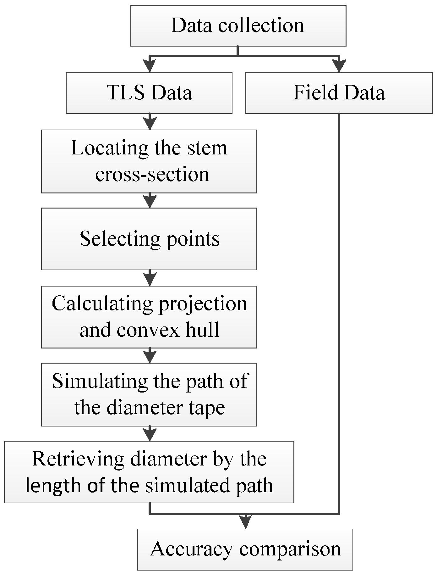
A flowchart showing the methodology used in this study is presented in
Figure 1. This section includes descriptions of the study tree species, field work and a series of procedures for simulating the path of the diameter tape to retrieve the stem diameter.
2.1. Study Materials
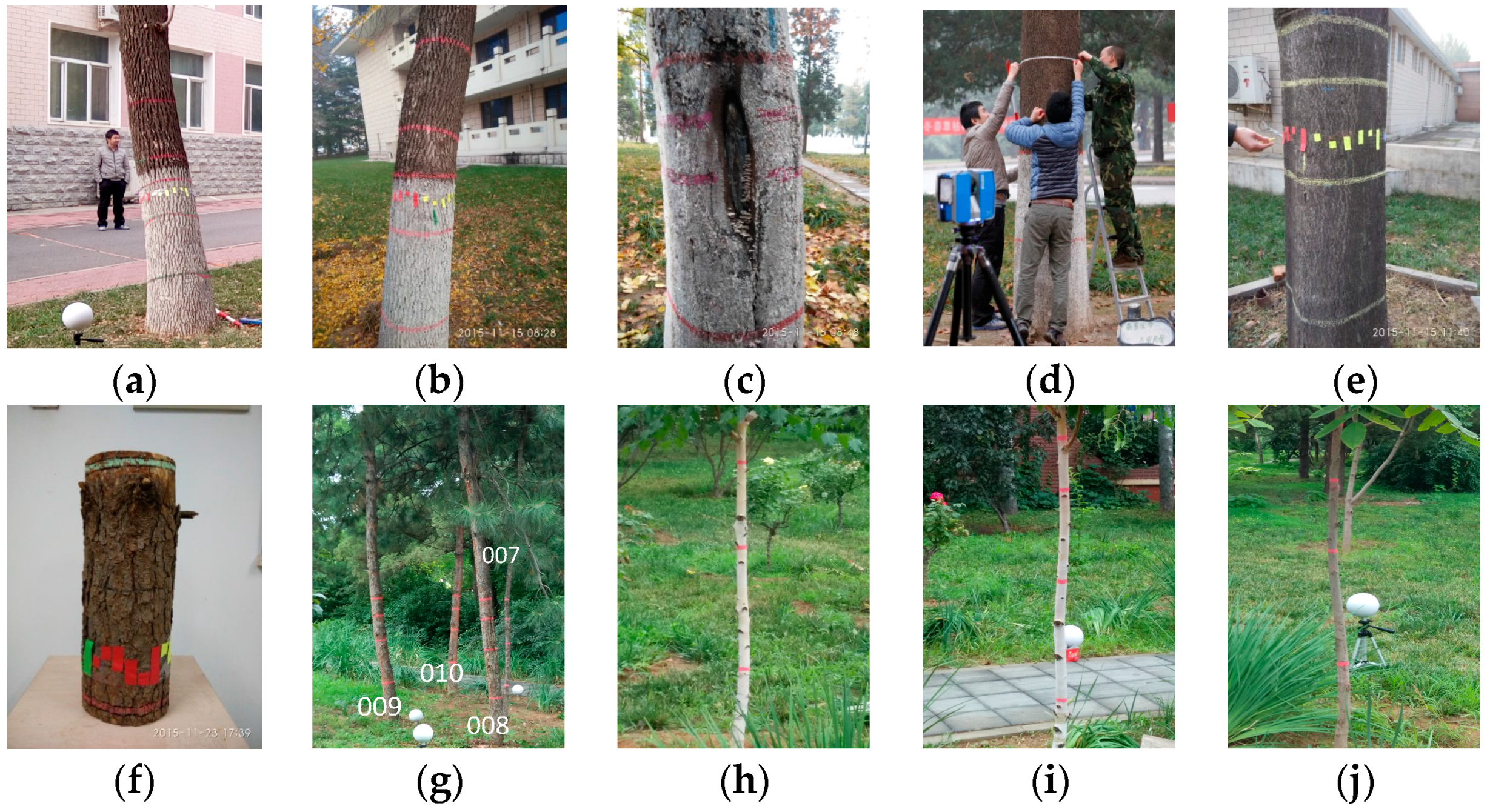
The study area was located in the courtyard of the Chinese Academy of Forestry. The field work was completed in November 2015 and July 2016. Twelve standing trees and one log belonging to eight different tree species were chosen as the study materials. The tree information is listed in
Table 2. In the field work, the stem diameter was manually measured using stainless steel diameter tape after the stem cross-section was determined. The stem cross-section can be evaluated by the perpendicularity between the path of the diameter tape and the stem axis. The path of the diameter tape was labelled with colored chalk (
Figure 2). Several diameters at different height positions of the standing trees were measured. A total of 57 records of stem diameter were obtained during the field work (
Table 2).
Four-directional scans of each tree were conducted using a FARO X330 terrestrial laser scanner. The scan quality was 4×; the scan resolution was ¼; the scan speed was 122 kpts/s (122 thousands points per second); and the point distance was 6.136 mm/10 m (the point distance describes the scan accuracy and refers to the distance between the two nearest captured scan points in mm at a scan distance of 10 m). For each standing tree, the horizontal distances from the tree to the scanner in different scan positions were between 8 and 10 m, and the distance from the scanner to the log was approximately 2.5 m (it was scanned in the room). The scanner was placed on the tripod, and the height of the scanner was approximately 1.2 m. The point cloud registration of the four scans and the extraction of the tree stem points were manually performed using the FARO Scene5.0 software.
2.2. Determining the Stem Cross-Section
The stem cross-section is the intersection between a plane and the tree stem. It should be perpendicular to the stem axis. For simplification, the plane of the stem cross-section is referred to as the stem cross-sectional plane.
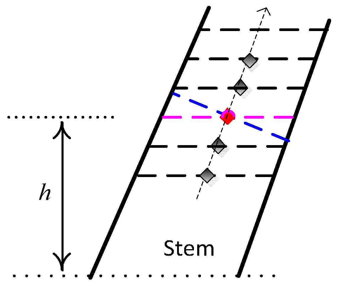
A stem does not have a regular geometry. Different stem cross-sections at different heights are not parallel. The stem cross-sectional planes at different heights along the stem should be determined individually. In this study, the stem cross-sectional plane at a given height h was determined by an anchor point and the growth direction of the stem at the given height. First, an anchor point P on the stem cross-section was located according to the height value and the given initial normal vector . Second, the applicable normal vector of the stem cross-section, which was equal to the growth direction of the stem, was calculated by iteration. Third, the stem cross-sectional plane was determined by the normal vector and the anchor point P.
2.2.1. Locating the Anchor Point of the Stem Cross-Section
The stem diameter usually refers to the diameter of the stem cross-section at a certain height along the stem. Given the irregular geometry of a stem, the different points on the same stem cross-section may have different height values. In this study, the height value of the stem was the vertical distance from the lowest point to the geometrical central point of the stem. The lowest point can be calculated from the stem points. An initial plane (
Figure 3) can be calculated based on the initial normal vector
, the lowest point and the height value
h. An upper plane was constructed above and parallel to the initial plane. The distance between the planes was 0.5 cm. Then, a stem slice was formed between the two planes. The anchor point (
Figure 3) was the geometric central point of the stem slices.
The irregularity of the stem cross-section yields a complicated geometrical shape of the stem slice. Additionally, the density of the stem points is uneven, and a stem may have concave surfaces. Considering the above factors, it is a challenge to accurately define the geometric central point of a stem slice. In this study, the geometric central point of a stem slice was represented by the centroid of the convex polygon that was formed from the planar projection point set, which is the resultant point set of the stem slice points projecting onto its lower stem cross-section.
2.2.2. Calculating the Growth Direction of the Stem
According to the above method of obtaining a stem slice, the other four stem slices can be obtained using parallel planes (
Figure 3). Two of the four stem slices was above the stem slice of the anchor point, and the other two planes were below the stem slice of the anchor point. Then, five geometric central points of the stem slices can be calculated. The growth direction of the stem is approximately equal to the maximum variation direction of the geometric central points of the stem slices. Then, the principal component analysis (PCA) method was used to calculate the growth direction. The eigenvector that corresponds to the greatest eigenvalue is the growth direction of the stem.
Obviously, the more parallel the relationship between the plane of the stem slice and the stem cross-section of the stem, the more accurate the derived growth direction. Hence, an iterative strategy was adopted. The
-th iteration is described as follows: the geometric central point
of the stem slices was calculated from the previous normal vector
. The normal value
was calculated from PCA and
. The iteration ended when the included angle
between
and
was less than 0.5 degrees or the absolute difference between the adjacent included angles
and
was less than 0.5 degrees. Then,
was the growth direction of the stem at the given height and the applicable normal vector
of the stem cross-section. Note that points of the stem slices may be changed during each iteration. The lower stem cross-section of the third stem slice in each iteration must pass through the anchor point to ensure the validity of the iteration (
Figure 3).
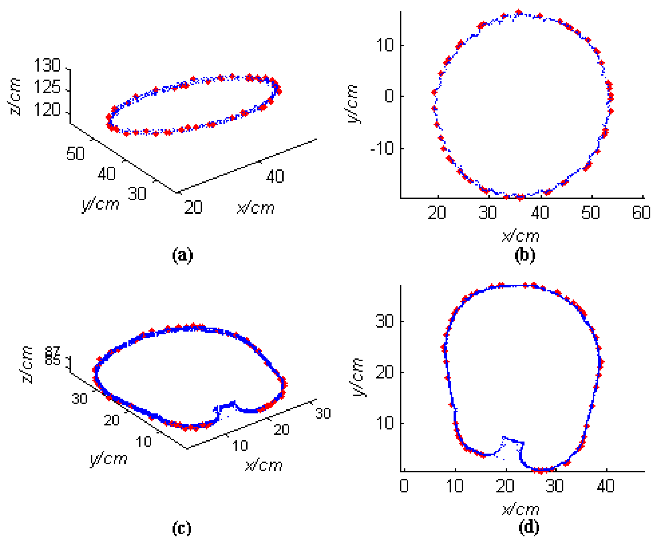
2.3. Selecting Points for Retrieving Stem Diameter
The point set that is used to retrieve stem diameter is denoted by P. The point set P can be selected after the stem cross-section is located. The point set P should be sourced from points of the stem cross-section. Because the distances from a target tree to the scanner are different in different scanner positions, the distribution of stem points is uneven. The points belonging only to a certain stem cross-section do not reflect the integral profile of the stem cross-section. Additionally, the path of the diameter tape has a constant width, which is equal to the width of the diameter tape. Thus, the point set P can be selected from a band of stem points between two parallel stem cross-sectional planes. The normal vectors of the two parallel stem cross-sectional planes are equal, and the distance between the two parallel stem cross-sectional planes is the width of the diameter tape. To avoid confusion, the thickness of the stem points used for extracting stem diameter was the distance between the two parallel stem cross-sectional planes and was referred to as the width of the band in this study.
In experiments of this study, for compatibility and comparison with the field-measured diameter in the field work, the point set
P should represent the colored points that consist only of the points on the path of the diameter tape. According to
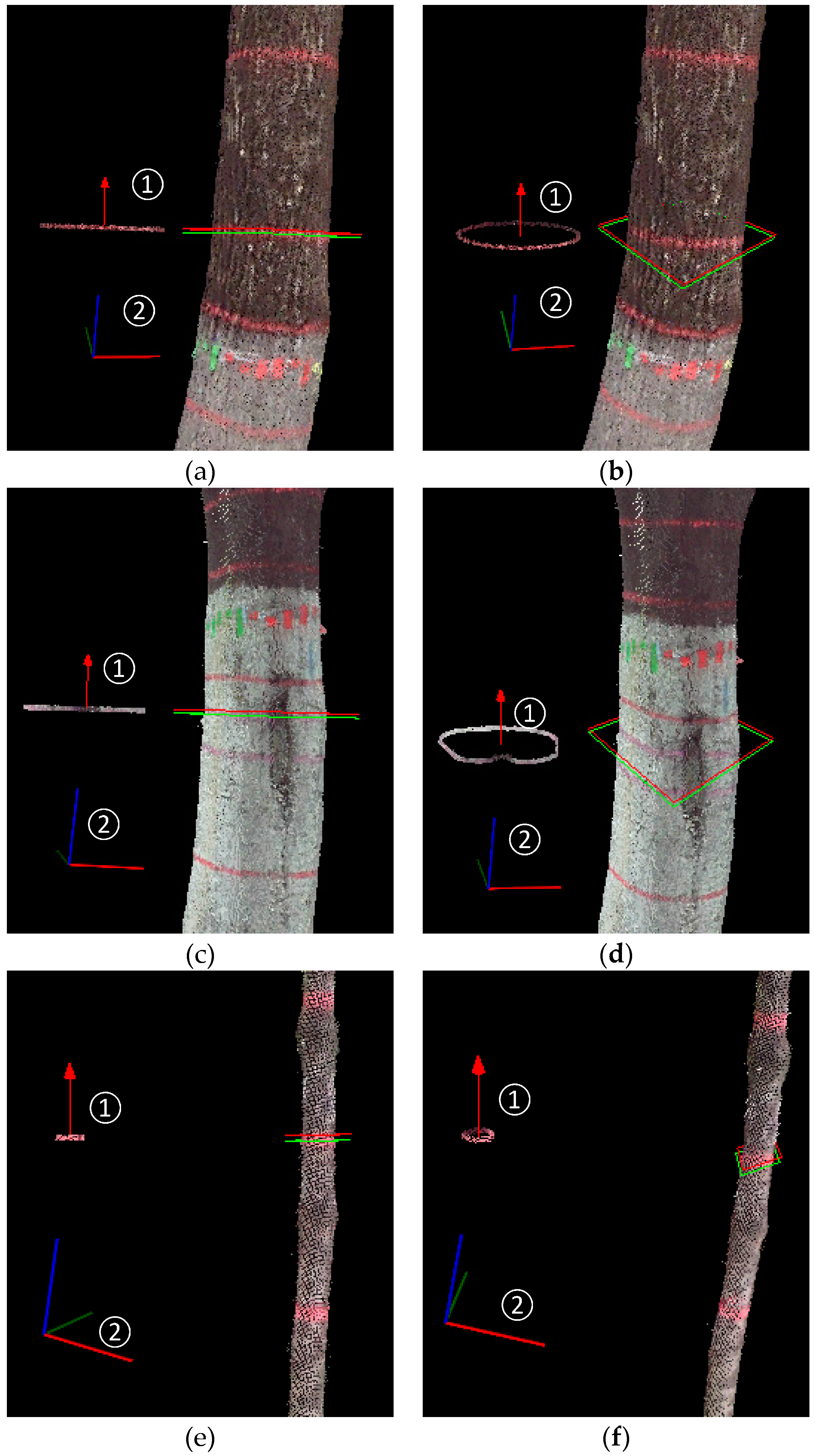
Section 2.2, the normal vector of the two parallel stem cross-sectional planes can be calculated, and the distance between the two parallel stem cross-sectional planes is equal to 1 cm, which is the width of the diameter tape. Then, the path of the diameter tape in the field work traces the area between the two parallel stem cross-sectional planes in the stem. The selected points of one path of the diameter tape of Tree 002 and Tree 003 are shown in
Figure 4.
2.4. Calculating the Projection and the Convex Hull
The thickness value of the stem points for calculating the stem diameter is the width value of the diameter tape. Direct simulation of the path of the diameter tape in three-dimensional space is difficult. However, the path of the diameter tape can be simplified as a closed curve. Then, the problem of simulating the path of the diameter tape can be considered as a problem of curve fitting. The path of the diameter tape is formed by the bulgy bark of the stem. The simulation path of the diameter tape should also adhere to this notion. The convex hull of the point set
X is the smallest convex set that contains
X. The bulgy bark of the stem can be considered to be the convex hull of the stem points. For more information about the convex hull, please refer to [
33].
In
Section 2.3, the point set
P that is used to calculate stem diameter was selected through two stem cross-sectional planes. Note that point set
P is a point set in three-dimensional space. The planar point set
Pprojection was obtained by projecting point set
P onto one of the two stem cross-sectional planes. Then, the convex hull points of the planar point set
Pprojection served as the interpolation points that were used for curve fitting to simulate the path of the diameter tape. The planar point set
Pprojection is also a point set in three-dimensional space. To simplify the computation, the point set
Pprojection can be converted to a planar point set
P’ in two-dimensional space by point rotating. Then, a simulated path of the diameter tape can be interpolated on the convex hull points of the planar point set
P’ in two-dimensional space. The convex hull points of the stem cross-section of
Figure 3 are shown in
Figure 5.
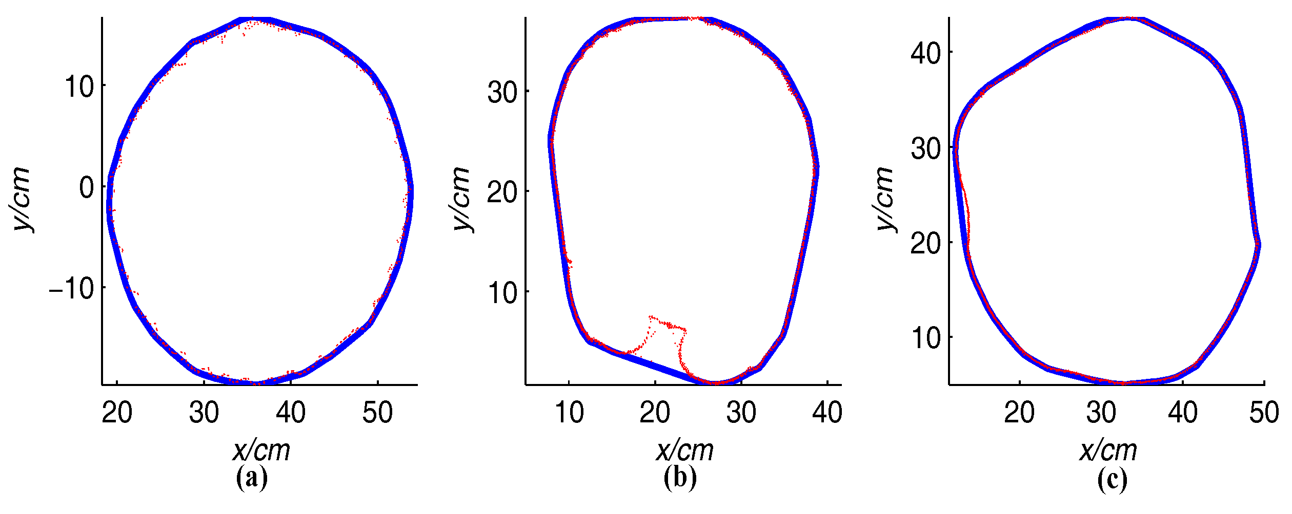
2.5. Simulating the Path of the Diameter Tape
The problem of simulating the path of the diameter tape can be described as follows: for a given convex hull point set Phull of the projected points in a two-dimensional space, a smooth closed curve, which passes through the points of Phull, can be constructed. This problem is a classic problem in computer graphics. A B-spline curve is a common method for curve fitting due to its superior properties. A cubic B-spline curve is a second-order geometric continuity curve; the path of the diameter tape also has the property of second-order geometric continuity. Thus, a closed smooth cubic non-rational B-spline curve was employed to simulate the path of the diameter tape in this study.
Three steps are required to construct a
-th non-rational B-spline curve to interpolate the points in
. The first step is to assign the parameter value
for each
. The construction of an appropriate non-decreasing knot vector
is the second step. Setting up and resolving the
system of linear equations is the third step. The linear equations can be described as:
where the control points
are the
n + 1 unknown points,
is the degree of B-spline curve and
is the
i-th of
-degree B-spline basis function. In this study, a recurrence formula presented by deBoor, Cox and Mansfield [
34] is employed as the B-spline basis function.
is defined as:
where
.
After the three steps, the
-th non-rational B-spline curve can be defined by:
The results of the
and knot vector
affect the shape and parameterization of the curve. Based on the experiment, the centripetal method [
35] for assigning the parameter value
for
and the averaging method [
34] for constructing the knot vector
were employed in this study.
The centripetal method is described as follows: Let:
Then, the parameter value:
The averaging method [
34] for constructing the knot vector
can be defined by:
When p = 3, a cubic non-rational B-spline curve that passes through the given points can be constructed. To construct a closed smooth cubic non-rational B-spline curve, the first point of is established as the landmark point. The first three points of are inserted at the rear of , whereas the last three points of are inserted at the head of . Then, a new point set is formed. The interpolating curve of the new will pass through the landmark point twice. The parameter values and are noted when the curve passes through the landmark point. A closed smooth curve will be obtained according to Formula (4) by replacing and with and .
The simulated paths of the diameter tape are shown in
Figure 6.
Figure 6a,b corresponds to the stem cross-section in
Figure 5a,c.
Figure 6c shows a simulated path of the diameter tape for Tree 005.
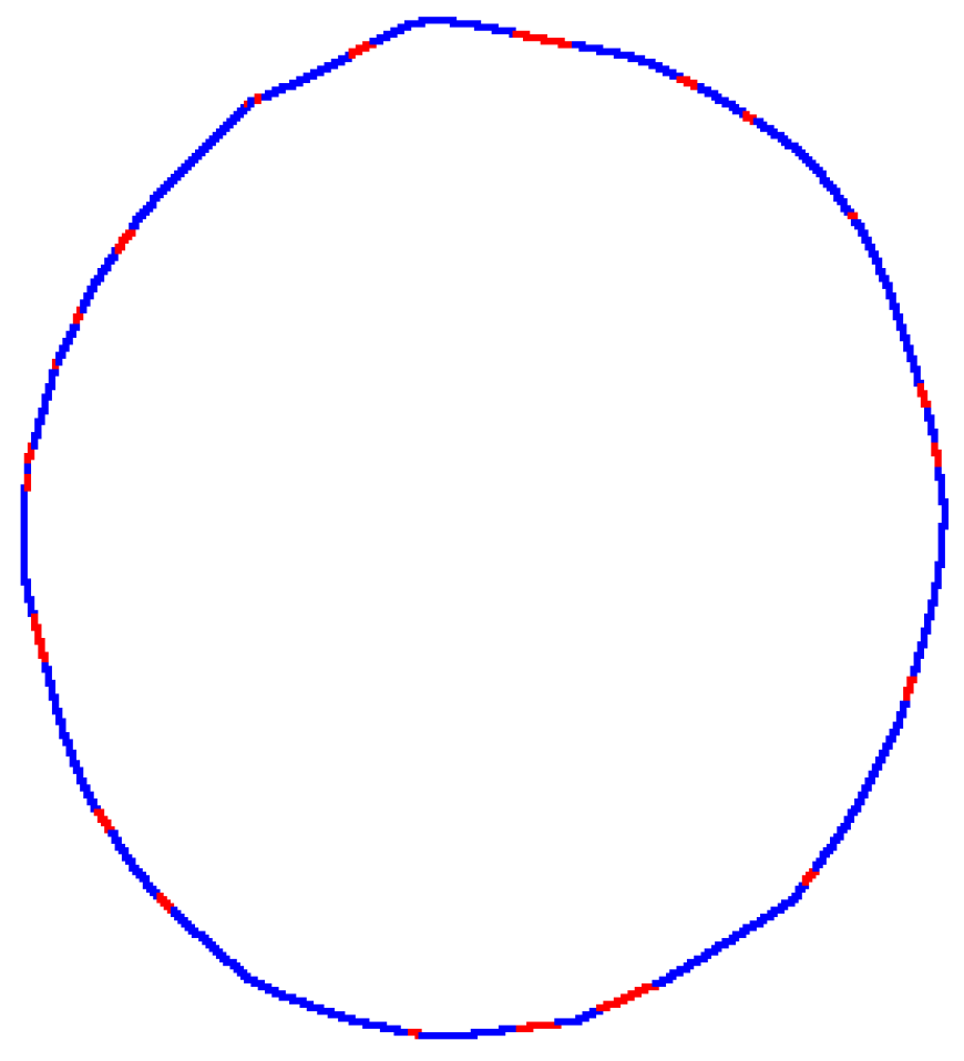
As shown in
Figure 6, the simulated path of the diameter tape was tightly wrapped around the outer points of the stem cross-section, and the concave region was overlooked. This condition conforms to the situation of stem diameter that was measured by the diameter tape in the field work.
2.6. Retrieving Stem Diameter
Stem diameter can be retrieved by the length of a closed smooth curve.
where
L is the length of the closed smooth curve and
D is the diameter value of the stem cross-section. In this study, the closed smooth curve is created by a cubic B-spline curve that is defined by several piecewise polynomial curves. Each section is a cubic polynomial curve. The length of each section can be solved by integrating. The formula of
can be rewritten as:
The length
s’ of the curve that extends between the parameter value
and
can be solved by:
In this study, , and are cubic polynomials. Thus, the primitive function of does not have an explicit solution. Thus, the length value of cannot be directly calculated. However, it can be indirectly calculated by the numerical integration of the composite Simpson’s rule. Please refer to the books about numerical integration to learn about the composite Simpson’s rule.
The implementation of the method presented in this study was based on the Point Cloud Library (PCL) [
36]. PCL is a standalone, large-scale, open source C++ library for 2D/3D image and point cloud processing.
4. Discussion
Although the existing methods focused on deriving DBH, this study focused on obtaining the diameter at multiple heights of the stem. The calculation of the DBH is similar to the calculation of the diameter at multiple heights of the stem. Their difference is the height position of the diameter. No difference was observed in calculating the diameter after locating the stem cross-section. Thus, the results of the existing method can be compared with the results of this study.
4.1. The Influence of Locating the Stem Cross-Section on Retrieving Stem Diameter
In theory, stem diameter and the stem cross-section are closely related. The stem diameter has local characteristics. The diameters of different positions along the stem are not identical. Even for a stem segment with a length of less than 5 cm, the difference in the diameter between the upper and the lower positions may be large. The points used to derive the stem diameter must be appropriately selected. In this study, the points used to derive the stem diameter were selected according to the cross-section and the width of the diameter tape. According to the experimental results, the accuracy of the circle fitting method was significantly improved. The maximum and minimum RMSE values of the circle fitting method, as listed in
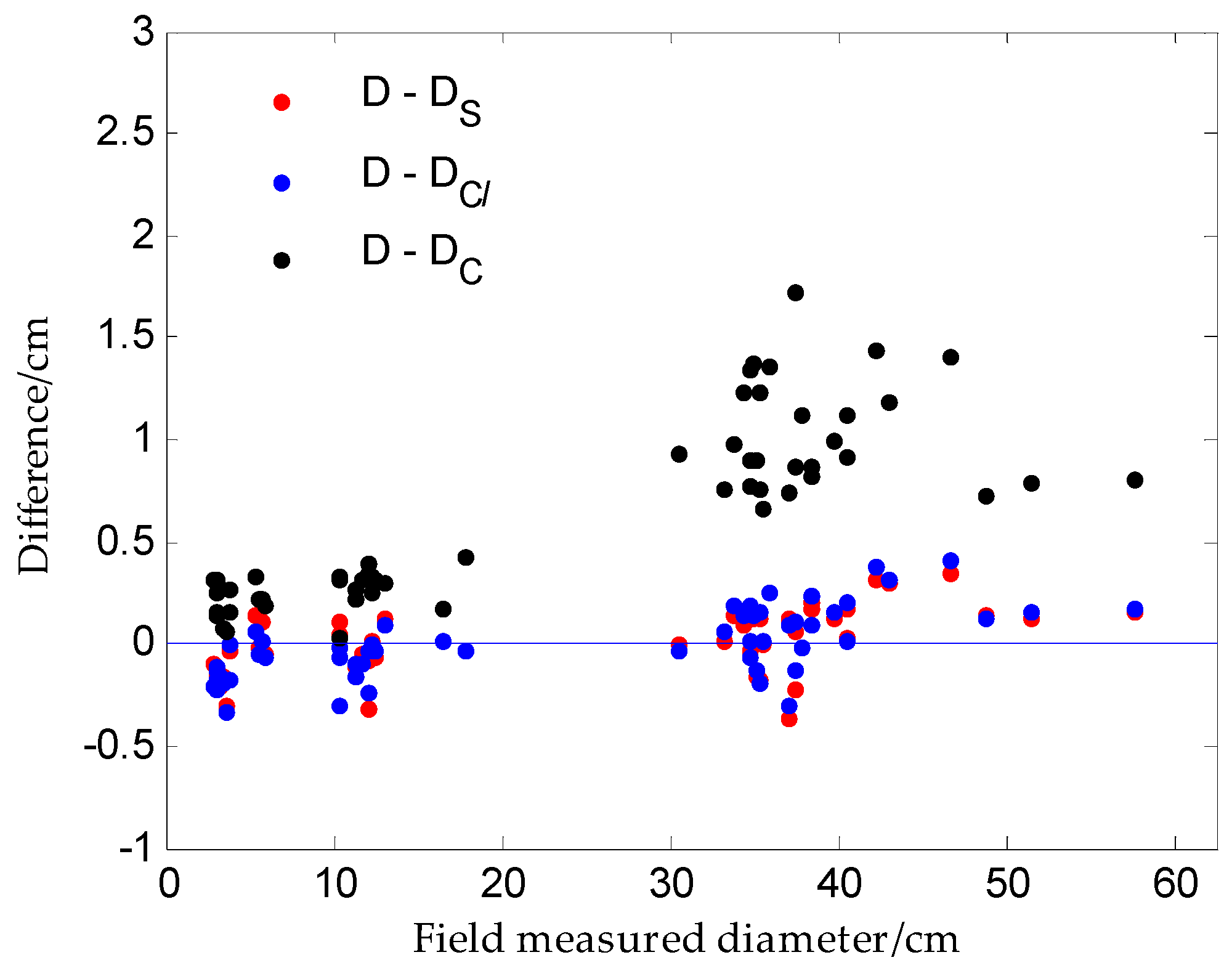
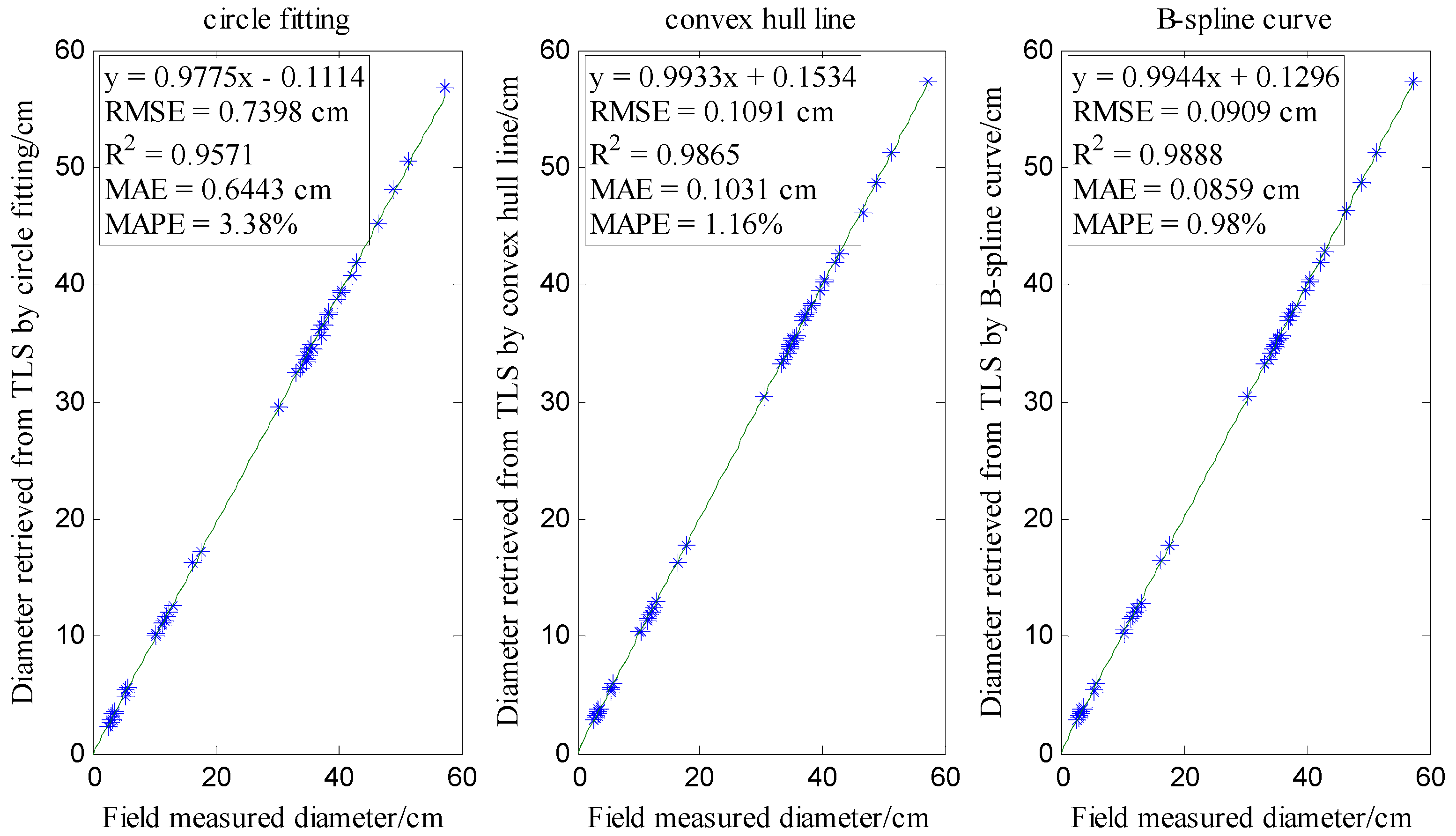
Table 1, were 4.2 cm and 1.8 cm. The RMSE value of the circle fitting method using the points of this study was 0.7398 cm. Compared with the RMSE value of the circle fitting method described in
Table 1, the RMSE value of the circle fitting method using the points of this study was significantly less. The importance of stem cross-section location for retrieving stem diameter is illustrated.
4.2. The Significance of Convex Hull Points for Retrieving Stem Diameter
In the field work, stem diameter is determined at the bulgy part of the stem. However, the majority of the existing methods seem to disregard this fact. The accuracies of these methods are thus not guaranteed. The convex hull line method accounts for this issue. Compared with the circle fitting method, the RMSE value of the convex hull line was nearly one eighth the RMSE value of the circle fitting method, as shown in
Figure 8. The accuracy of the diameter derived by the convex hull is significantly greater than that of the circle fitting method. The significance of the convex hull points for retrieving stem diameter is illustrated.
4.3. Applicability of the Method to Forestry
The path of the diameter tape is formed on the bulgy part of the stem cross-section. The bulgy part of the stem cross-section was reflected by the convex hull points of the stem cross-sectional points. Solving convex hull points of a given point cloud is a computation geometry problem. Once a point cloud is determined, the convex hull points of the point cloud are also determined. The main factors affecting the accuracy of stem diameter retrieval includes locating the stem cross-section and stem point set selection for retrieving stem diameter. In this study, the selection of the stem point set was based on the stem cross-section, and the thickness was the width of the diameter tape. Hence, stem diameter can be accurately retrieved from the stem cross-section. The procedure by which the stem cross-section was determined based on the relationships among the five geometric central points of the five successive stem slices. The iterative procedure can ensure the validity of the normal vector of the stem cross-sectional plane. The geometric central point of the stem slice was based on the convex hull points of the stem slice.
According to the above, the calculations in this study were based on the methodology of the field diameter measured by diameter tape and geometric computations. In fact, the stem point cloud is a version of a stem image. After a stem point cloud has been obtained and the profile of the stem has been reflected, the diameter can be obtained by the methods described in this study. The influences of the roughness of the stem bark, surface defects in the stem, the tilt degree of the stem and the height at the measured position were eliminated by the calculation of convex hull points and the iteration of the normal vector of the stem cross-sectional plane. Our findings were also supported by the experimental results. Similarly, the influence of the size of the stem diameter can also be eliminated. The maximum and minimum values of the stem diameter in this study were 57.4 and 2.7 cm, respectively. Although a smaller and a larger stem were not included, the calculations used in this study, which are based on the geometric characteristics, ensure the validity of stem diameters retrieval for smaller stems and larger stems.
The location of the cross-section is not considered in the existing methods. However, the convex hull line method is based on the convex hull points of the stem. The convex hull line does not meet the condition of geometry continuity. Thus, the accuracy of the existing methods is less than the accuracy of the method presented in this study.
4.4. Future Work
As described in
Figure 10, the simulated path of diameter tape is a global convex curve. Construction of a closed smooth and global convex curve to simulate the path of diameter tape is recommended for future studies.
The thickness of the stem points used in calculations of stem diameter was equal to the width of the diameter tape. The width of a diameter tape is usually 1 cm. The number of points is related to the density of the stem point cloud. When the density of the stem point cloud is sparse, the stem cross-section may not be reflected by the points with a thickness of 1 cm. The method requires a dense stem point cloud. The appropriate density of the stem point cloud to facilitate deriving the diameter from the stem point cloud is an important topic for future research.
Although TLS is not an instrument for routine forest inventory yet, it can provide the geometrical structure of the trees. On the basis of these geometrical structures, accurate stem diameter, stem basal area and stem volume can be calculated using geometric computations and mathematics. The algorithm of this study was designed for retrieving stem diameters at multiple heights along the stem. Accurate calculation of the stem basal area and stem volume requires further research. Improving and applying the algorithm of this study to standing forests is another important topic for future research.
5. Conclusions
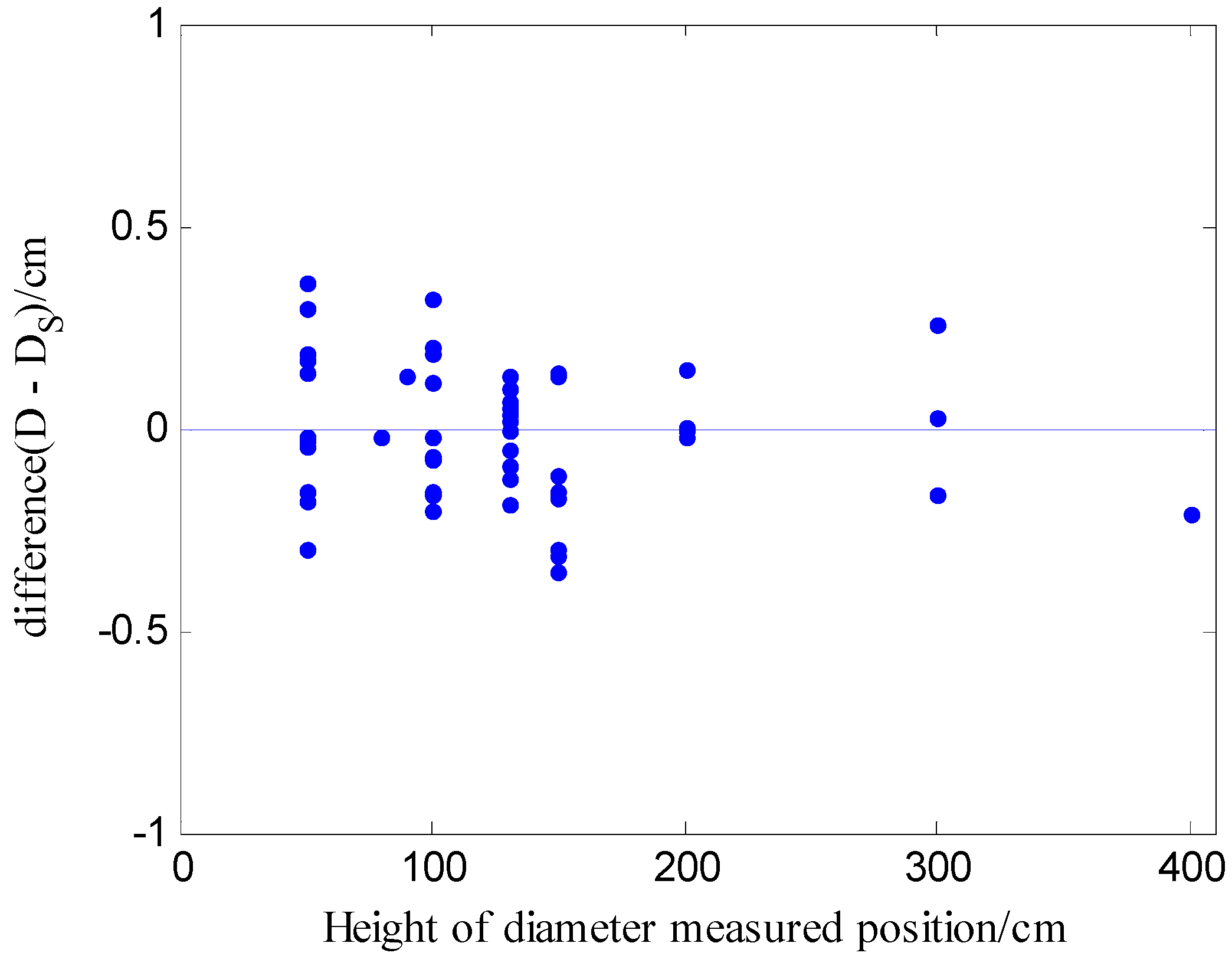
A novel algorithm for retrieving the stem diameter by simulating the path of the diameter tape is presented in this study. There are three steps in the algorithm: automatic determination of the stem cross-section at a given height along the stem; choice of the stem points from which to retrieve stem diameter and the simulation of the path of the diameter tape. Calculation of the algorithm based on the definition of stem diameter and obeying the diameter measurement rules in forest inventory. The experimental data were collected from different stem forms and tree species. Compared with the diameter measured in the field work, the RMSE values of circle fitting, convex hull line and simulating the path of diameter tape by the B-spline curve were 0.7398, 0.1091 and 0.0909 cm, respectively. The importance of stem points’ selection to retrieve the stem diameter and the applicability of the method were discussed.
The RMSE value of the method presented in this study satisfies the accuracy requirement in forest inventory. This study demonstrated that accurate determination of the stem cross-section is important for retrieving the stem diameter and that stem diameters retrieved from TLS can exhibit millimeter-level accuracy for individual trees. The study also describes the thickness of stem points needed to retrieve the stem diameter and provides an efficient and precise method for deriving the stem diameter from TLS data. Future studies should investigate the applicability of the algorithm to retrieving the stem diameter in forest stands.


 ,
, 


