
Mapping Forest Health Using Spectral and Textural Information Extracted from SPOT-5 Satellite Images


Abstract
:
1. Introduction
2. Data and Methods
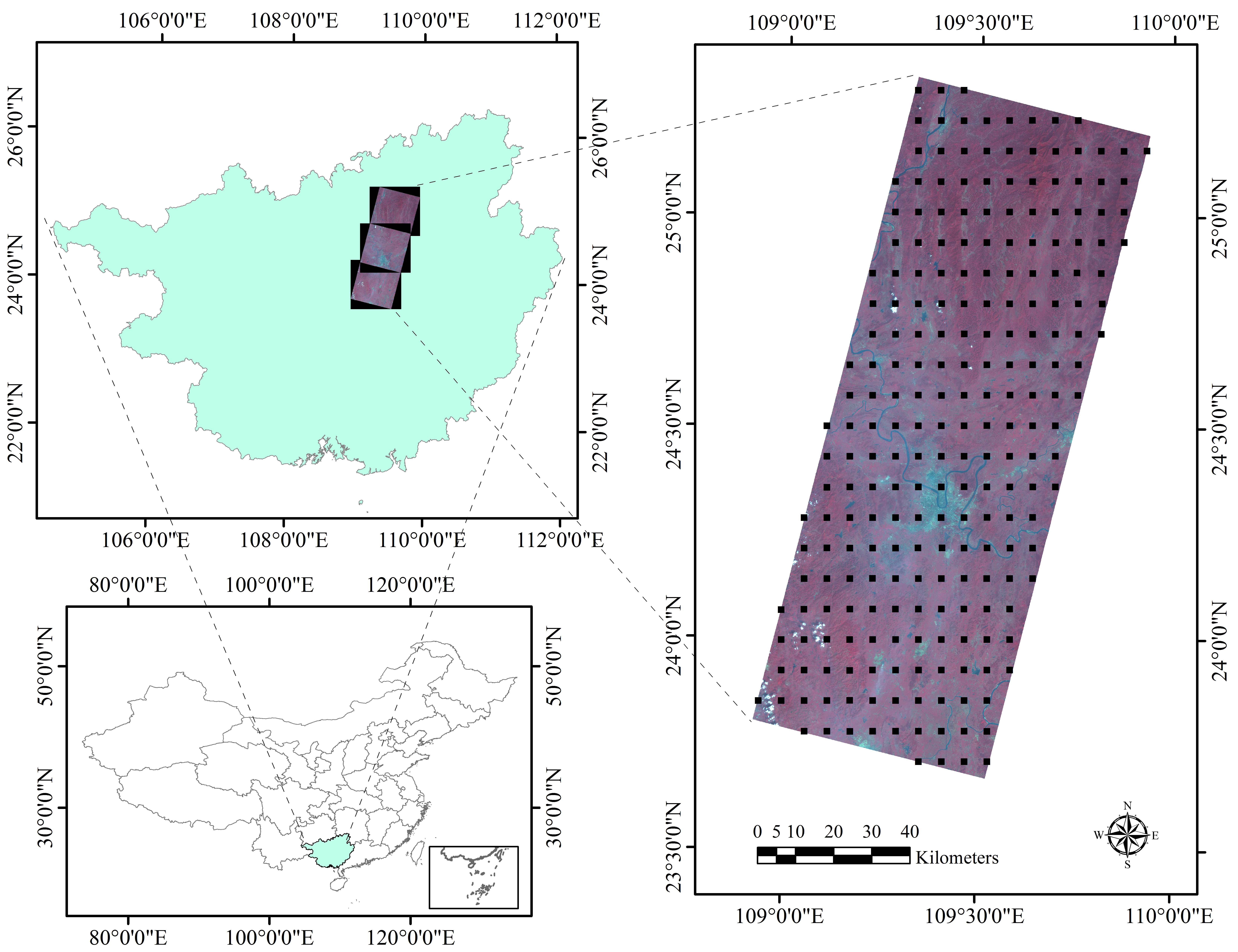
2.1. Data Source
2.1.1. Field Data
2.1.2. Remote Sensing Data and Processing
2.2. Forest Health Indicator
2.2.1. Forest Stand Attributes for Calculating the Forest Health Indicator
2.2.2. Forest Health Indicator Derivation
2.3. Imagery-Derived Measures
2.3.1. Spectral Measures
2.3.2. Textural Measures
2.4. Statistical Methods
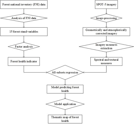
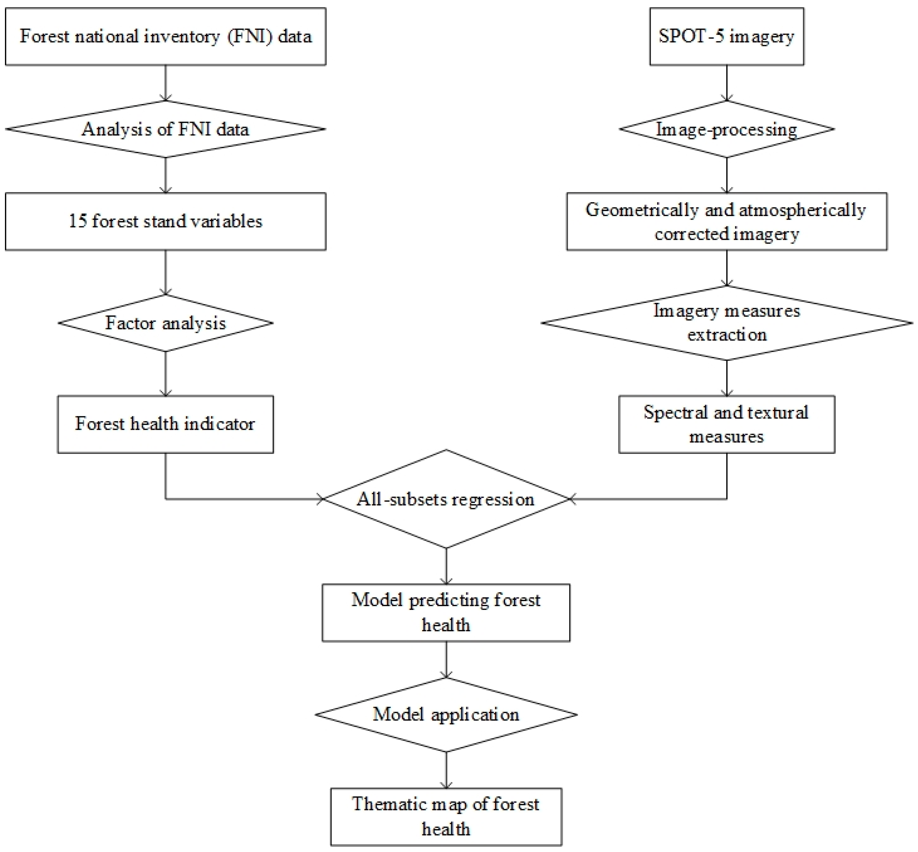
2.5. Experimental Procedure
3. Results
3.1. Forest Health Indicator Derivation
3.2. Correlation Analyses
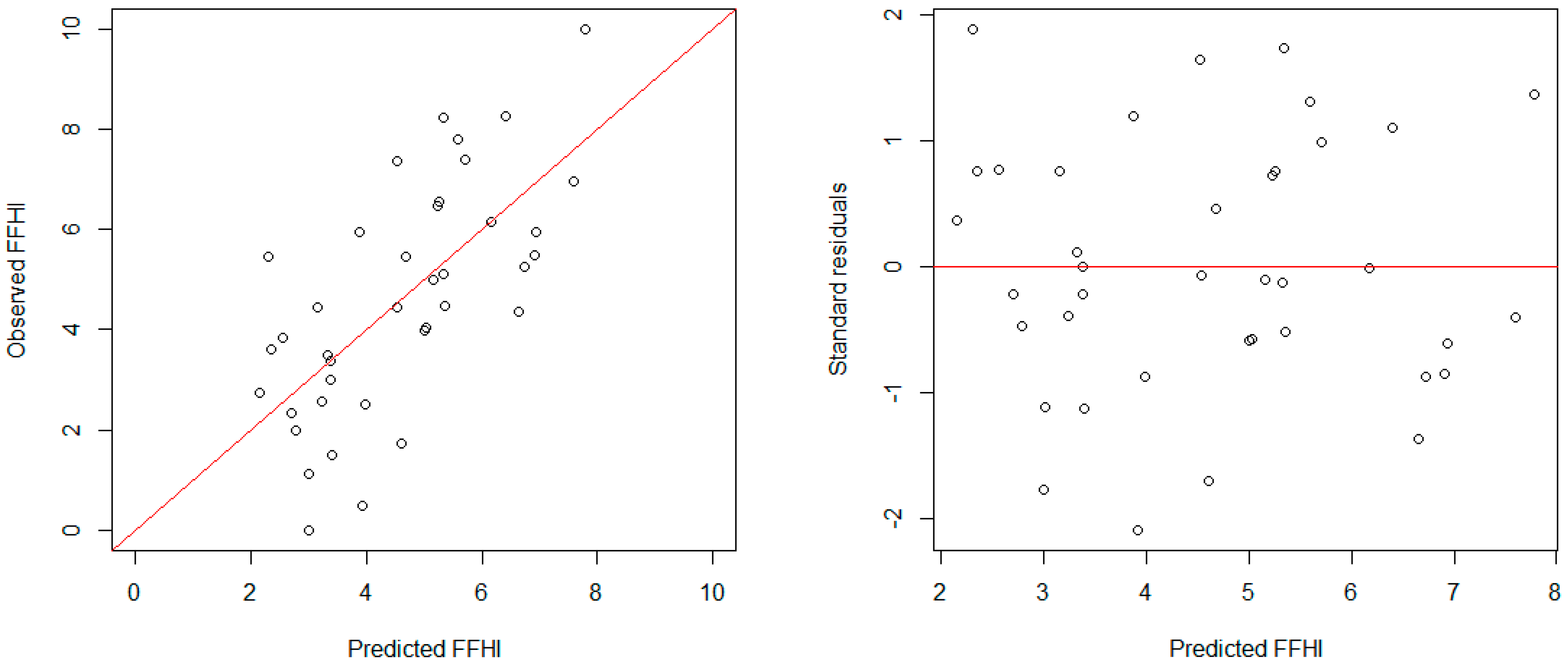
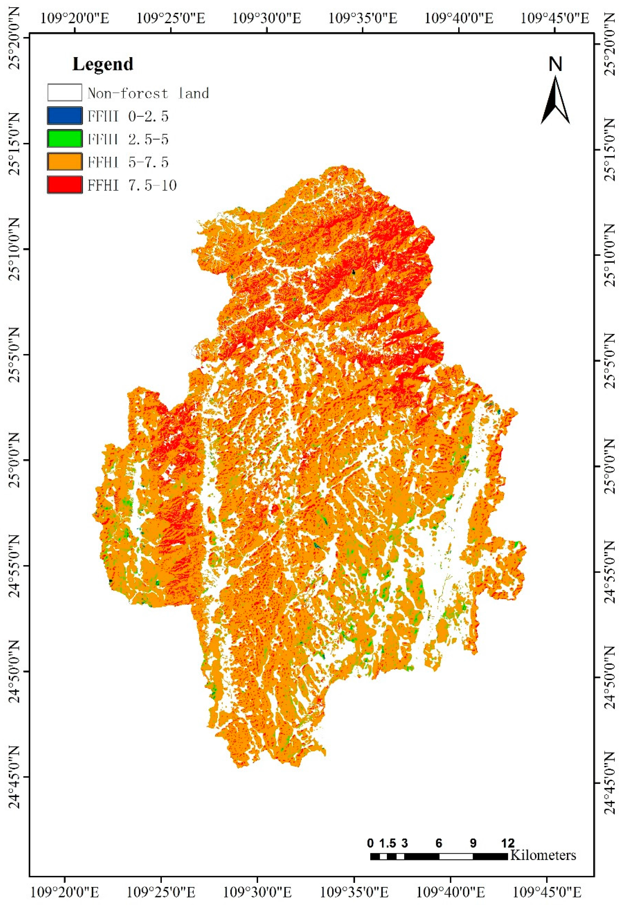
3.3. Model Establishment and Forest Health Mapping
4. Discussion
4.1. Forest Health Indicator Derivation
4.2. Predictive Model Development
4.3. Implication for Forest Management
5. Conclusions
Acknowledgments
Author Contributions
Conflicts of Interest
References
- Davis, L.S.; Norman Johnson, K.; Bettinger, P.S.; Howard, T.E.; Alván Encinas, L.; Salazar, M.; Gretzinger, S.; Lange, G.; Schmithusen, F.; Hyde, W.; et al. Forest Management: To Sustain Ecological, Economic, and Social Values; Universidad Nacional Agraria La Molina: Lima, Perú, 2001. [Google Scholar]
- Buschbacher, R.J. Natural forest management in the humid tropics: Ecological, social, and economic considerations. Ambio (Sweden) 1990, 19, 253–258. [Google Scholar]
- Pfilf, R.J.; Marker, J.; Averill, R.D. Forest Health and Fire: An Overview and Evaluation; National Association of Forest Service Retirees: Fort Collins, CO, USA, 2002. [Google Scholar]
- Meng, J.; Lu, Y.; Zeng, J. Transformation of a degraded pinus massoniana plantation into a mixed-species irregular forest: Impacts on stand structure and growth in southern China. Forests 2014, 5, 3199–3221. [Google Scholar] [CrossRef]
- Knoke, T.; Ammer, C.; Stimm, B.; Mosandl, R. Admixing broadleaved to coniferous tree species: A review on yield, ecological stability and economics. Eur. J. For. Res. 2008, 127, 89–101. [Google Scholar] [CrossRef]
- Redondo-Brenes, A.; Montagnini, F. Growth, productivity, aboveground biomass, and carbon sequestration of pure and mixed native tree plantations in the caribbean lowlands of Costa Rica. For. Ecol. Manag. 2006, 232, 168–178. [Google Scholar] [CrossRef]
- O’Hara, K.L. The silviculture of transformation—A commentary. For. Ecol. Manag. 2001, 151, 81–86. [Google Scholar] [CrossRef]
- Puettmann, K.J.; Wilson, S.M.; Baker, S.C.; Donoso, P.J.; Drössler, L.; Amente, G.; Harvey, B.D.; Knoke, T.; Lu, Y.; Nocentini, S.; et al. Silvicultural alternatives to conventional even-aged forest management—What limits global adoption? For. Ecosyst. 2015, 2, 1–16. [Google Scholar] [CrossRef]
- Filotas, E.; Parrott, L.; Burton, P.J.; Chazdon, R.L.; Coates, K.D.; Coll, L.; Haeussler, S.; Martin, K.; Nocentini, S.; Puettmann, K.J.; et al. Viewing forests through the lens of complex systems science. Ecosphere 2014, 5, 1–23. [Google Scholar] [CrossRef]
- Waring, R.H. Forest, fresh perspectives from ecosystem analysis. In Vital Signs of Forest Ecosystems; Oregon State University Press: Corvallis, OR, USA, 1980; pp. 131–136. [Google Scholar]
- Smith, W.H. Health of north american forests: Stress and risk assessment. J. For. USA 1990, 88. [Google Scholar]
- O’Laughlin, J.; Cook, P.S. Inventory-based forest health indicators: Implications for national forest management. J. For. 2003, 101, 11–17. [Google Scholar]
- Tuominen, J.; Haapanen, R.; Lipping, T.; Kuosmanen, V. Remote Sensing of Forest Health; INTECH Open Access Publisher: Rijeka, Croatia, 2009. [Google Scholar]
- Lim, S.S. Development of Forest Aesthetic Indicators in Sustainable Forest Management Standards; University of British Columbia: Vancouver, BC, Canada, 2012. [Google Scholar]
- Turnblom, K.W. Private Forests in The Wildland-Urban Interface: Using Geographic Information Systems (GIS) to Identify Management Challenges in Eastern Washington, United States. Master’s Thesis, Utah State University, Logan, UT, USA, 2015. [Google Scholar]
- Lorenz, M. International co-operative programme on assessment and monitoring of air pollution effects on forests-ICP forests. Water Air Soil Pollut. 1995, 85, 1221–1226. [Google Scholar] [CrossRef]
- Alexander, S.A.; Palmer, C.J. Forest health monitoring in the united states: First four years. Environ. Monit. Assess. 1999, 55, 267–277. [Google Scholar] [CrossRef]
- D’Eon, S.; Magasi, L.; Lachance, D.; DesRochers, P. Canada’s National Forest Health Monitoring Plot Network Manual on Plot Establishment and Monitoring (Revised); Petawawa National Forestry Institute: Ontario, CA, USA, 1994. [Google Scholar]
- Crown Indicator Homepage. Available online: http://srsfia2.fs.fed.us/crowns/ (accessed on 11 April 2016).
- Wang, H.; Zhao, Y.; Pu, R.; Zhang, Z. Mapping Robinia pseudoacacia forest health conditions by using combined spectral, spatial, and textural information extracted from IKONOS imagery and random forest classifier. Remote Sens. 2015, 7, 9020–9044. [Google Scholar] [CrossRef]
- Wang, Y.; Solberg, S.; Yu, P.; Myking, T.; Vogt, R.D.; Du, S. Assessments of tree crown condition of two masson pine forests in the acid rain region in South China. For. Ecol. Manag. 2007, 242, 530–540. [Google Scholar] [CrossRef]
- Zarnoch, S.J.; Bechtold, W.A.; Stolte, K. Using crown condition variables as indicators of forest health. Can. J. For. Res. 2004, 34, 1057–1070. [Google Scholar] [CrossRef]
- Schomaker, M.E.; Zarnoch, S.J.; Bechtold, W.A.; Latelle, D.J.; Burkman, W.G.; Cox, S.M. Crown-Condition Classification: A Guide to Data Collection and Analysis; US Department of Agriculture, Forest Service, Southern Research Station: Asheville, NC, USA, 2007.
- O’Neill, K.P.; Amacher, M.C.; Perry, C.H. Soils as An Indicator of Forest Health; United States Forest Service, North Central Research Station: St. Paul, MN, USA, 2005.
- McCune, B. Lichen communities as indicators of forest health. Bryologist 2000, 103, 353–356. [Google Scholar] [CrossRef]
- Egli, S. Mycorrhizal mushroom diversity and productivity—An indicator of forest health? Ann. For. Sci. 2011, 68, 81–88. [Google Scholar] [CrossRef]
- Hilty, J.; Merenlender, A. Faunal indicator taxa selection for monitoring ecosystem health. Biol. Conserv. 2000, 92, 185–197. [Google Scholar] [CrossRef]
- Zhang, J.; Huang, S.; Hogg, E.; Lieffers, V.; Qin, Y.; He, F. Estimating spatial variation in alberta forest biomass from a combination of forest inventory and remote sensing data. Biogeosciences 2014, 11, 2793–2808. [Google Scholar] [CrossRef] [Green Version]
- Andersen, H.-E.; Strunk, J.; Temesgen, H.; Atwood, D.; Winterberger, K. Using multilevel remote sensing and ground data to estimate forest biomass resources in remote regions: A case study in the boreal forests of Interior Alaska. Can. J. Remote Sens. 2012, 37, 596–611. [Google Scholar] [CrossRef]
- Du, L.; Zhou, T.; Zou, Z.; Zhao, X.; Huang, K.; Wu, H. Mapping forest biomass using remote sensing and national forest inventory in China. Forests 2014, 5, 1267–1283. [Google Scholar] [CrossRef]
- Powers, R.P.; Coops, N.C.; Morgan, J.L.; Wulder, M.A.; Nelson, T.A.; Drever, C.R.; Cumming, S.G. A remote sensing approach to biodiversity assessment and regionalization of the Canadian boreal forest. Progr. Phys. Geogr. 2013, 37, 36–62. [Google Scholar] [CrossRef]
- Gairola, S.; Procheş, Ş.; Rocchini, D. High-resolution satellite remote sensing: A new frontier for biodiversity exploration in Indian Himalayan forests. Int. J. Remote Sens. 2013, 34, 2006–2022. [Google Scholar] [CrossRef]
- Laurin, G.V.; Chan, J.C.-W.; Chen, Q.; Lindsell, J.A.; Coomes, D.A.; Guerriero, L.; Del Frate, F.; Miglietta, F.; Valentini, R. Biodiversity mapping in a tropical West African forest with airborne hyperspectral data. PLoS ONE 2014, 9, e97910. [Google Scholar]
- Getzin, S.; Wiegand, K.; Schöning, I. Assessing biodiversity in forests using very high-resolution images and unmanned aerial vehicles. Method. Ecol. Evol. 2012, 3, 397–404. [Google Scholar] [CrossRef]
- Peduzzi, A.; Wynne, R.H.; Fox, T.R.; Nelson, R.F.; Thomas, V.A. Estimating leaf area index in intensively managed pine plantations using airborne laser scanner data. For.Ecol. Manag. 2012, 270, 54–65. [Google Scholar] [CrossRef]
- Liu, Q.; Liang, S.; Xiao, Z.; Fang, H. Retrieval of leaf area index using temporal, spectral, and angular information from multiple satellite data. Remote Sens. Environ. 2014, 145, 25–37. [Google Scholar] [CrossRef]
- Gao, F.; Anderson, M.C.; Kustas, W.P.; Houborg, R. Retrieving leaf area index from landsat using MODIS LAI products and field measurements. IEEE Geosci. Remote Sens. Lett. 2014, 11, 773–777. [Google Scholar]
- Jensen, J.; Qiu, F.; Ji, M. Predictive modelling of coniferous forest age using statistical and artificial neural network approaches applied to remote sensor data. Inter. J. Remote Sens. 1999, 20, 2805–2822. [Google Scholar]
- Dye, M.; Mutanga, O.; Ismail, R. Combining spectral and textural remote sensing variables using random forests: Predicting the age of Pinus patula forests in Kwazulu-Natal, South Africa. J. Spat. Sci. 2012, 57, 193–211. [Google Scholar] [CrossRef]
- Tooke, T.R.; Coops, N.C.; Webster, J. Predicting building ages from lidar data with random forests for building energy modeling. Energy Build. 2014, 68, 603–610. [Google Scholar] [CrossRef]
- Donoghue, D.; Watt, P. Using Lidar to compare forest height estimates from IKONOS and Landsat ETM+ data in Sitka spruce plantation forests. Int. J. Remote Sens. 2006, 27, 2161–2175. [Google Scholar] [CrossRef]
- Naesset, E. Determination of mean tree height of forest stands using airborne laser scanner data. ISPRS J. Photogramm. Remote Sens. 1997, 52, 49–56. [Google Scholar] [CrossRef]
- Næsset, E.; Økland, T. Estimating tree height and tree crown properties using airborne scanning laser in a boreal nature reserve. Remote Sens. Environ. 2002, 79, 105–115. [Google Scholar] [CrossRef]
- McCombs, J.W.; Roberts, S.D.; Evans, D.L. Influence of fusing lidar and multispectral imagery on remotely sensed estimates of stand density and mean tree height in a managed loblolly pine plantation. For. Sci. 2003, 49, 457–466. [Google Scholar]
- Wilkinson, G.; Folving, S.; Kanellopoulos, I.; McCormick, N.; Fullerton, K.; Megier, J. Forest mapping from multi-source satellite data using neural network classifiers—An experiment in Portugal. Remote Sens. Rev. 1995, 12, 83–106. [Google Scholar] [CrossRef]
- Van Coillie, F.M.; Verbeke, L.P.; De Wulf, R.R. Feature selection by genetic algorithms in object-based classification of IKONOS imagery for forest mapping in Flanders, Belgium. Remote Sens. Environ. 2007, 110, 476–487. [Google Scholar] [CrossRef]
- Pax-Lenney, M.; Woodcock, C.E.; Macomber, S.A.; Gopal, S.; Song, C. Forest mapping with a generalized classifier and Landsat TM data. Remote Sens. Environ. 2001, 77, 241–250. [Google Scholar] [CrossRef]
- Gjertsen, A.K. Accuracy of forest mapping based on Landsat TM data and a KNN-based method. Remote Sens. Environ. 2007, 110, 420–430. [Google Scholar] [CrossRef]
- Hyde, P.; Dubayah, R.; Peterson, B.; Blair, J.; Hofton, M.; Hunsaker, C.; Knox, R.; Walker, W. Mapping forest structure for wildlife habitat analysis using waveform lidar: Validation of montane ecosystems. Remote Sens. Environ. 2005, 96, 427–437. [Google Scholar] [CrossRef]
- Chuvieco, E.; Congalton, R.G. Application of remote sensing and geographic information systems to forest fire hazard mapping. Remote Sens. Environ. 1989, 29, 147–159. [Google Scholar] [CrossRef]
- Dubayah, R.; Sheldon, S.; Clark, D.; Hofton, M.; Blair, J.; Hurtt, G.; Chazdon, R. Estimation of tropical forest height and biomass dynamics using lidar remote sensing at La Selva, Costa Rica. J. Geophys. Res. Biogeosci. 2010, 115. [Google Scholar] [CrossRef]
- Nilsson, M. Estimation of tree heights and stand volume using an airborne lidar system. Remote Sens. Environ. 1996, 56, 1–7. [Google Scholar] [CrossRef]
- Simard, M.; Pinto, N.; Fisher, J.B.; Baccini, A. Mapping forest canopy height globally with spaceborne lidar. J. Geophys. Res. Biogeosci. 2011, 116. [Google Scholar] [CrossRef]
- Wolter, P.T.; Townsend, P.A.; Sturtevant, B.R. Estimation of forest structural parameters using 5 and 10 meter SPOT-5 satellite data. Remote Sens. Environ. 2009, 113, 2019–2036. [Google Scholar] [CrossRef]
- Wallis, C.I.; Paulsch, D.; Zeilinger, J.; Silva, B.; Fernández, G.F.C.; Brandl, R.; Farwig, N.; Bendix, J. Contrasting performance of lidar and optical texture models in predicting avian diversity in a tropical mountain forest. Remote Sens. Environ. 2016, 174, 223–232. [Google Scholar] [CrossRef]
- Maack, J.; Kattenborn, T.; Ewald Fassnacht, F.; Enssle, F.; Hernández Palma, J.; Corvalán Vera, P.; Koch, B. Modeling forest biomass using Very-High-Resolution data—Combining textural, spectral and photogrammetric predictors derived from spaceborne stereo images. Eur. J. Remote Sens. 2015, 48, 245–261. [Google Scholar] [CrossRef]
- Meng, S.; Pang, Y.; Zhang, Z.; Jia, W.; Li, Z. Mapping aboveground biomass using texture indices from aerial photos in a temperate forest of northeastern China. Remote Sens. 2016, 8, 230. [Google Scholar] [CrossRef]
- Castillo-Santiago, M.A.; Ricker, M.; de Jong, B.H. Estimation of tropical forest structure from SPOT-5 satellite images. Int. J. Remote Sens. 2010, 31, 2767–2782. [Google Scholar] [CrossRef]
- Lexerød, N.L.; Eid, T. An evaluation of different diameter diversity indices based on criteria related to forest management planning. For. Ecol. Manag. 2006, 222, 17–28. [Google Scholar] [CrossRef]
- Bettinger, P.; Tang, M. Tree-level harvest optimization for structure-based forest management based on the species mingling index. Forests 2015, 6, 1121–1144. [Google Scholar] [CrossRef]
- Ozdemir, I.; Karnieli, A. Predicting forest structural parameters using the image texture derived from Worldview-2 multispectral imagery in a dryland forest, Israel. Int. J. Appl. Earth Obs. Geoinf. 2011, 13, 701–710. [Google Scholar] [CrossRef]
- Pommerening, A. Approaches to quantifying forest structures. Forestry 2002, 75, 305–324. [Google Scholar] [CrossRef]
- Meng, J.; Li, S.; Wang, W.; Liu, Q.; Xie, S.; Ma, W. Estimation of forest structural diversity using the spectral and textural information derived from SPOT-5 satellite images. Remote Sens. 2016, 8, 125. [Google Scholar] [CrossRef]
- Bartlett, M.S. Tests of significance in factor analysis. Br. J. Stat. Psychol. 1950, 3, 77–85. [Google Scholar] [CrossRef]
- Kaiser, H.F. An index of factorial simplicity. Psychometrika 1974, 39, 31–36. [Google Scholar] [CrossRef]
- Germany, T. Object features: Layer values. In Ecognition Developer 7 Reference Book; Trimble Germany: Munich, Germany, 2011; pp. 262–272. [Google Scholar]
- Wallner, A.; Elatawneh, A.; Schneider, T.; Knoke, T. Estimation of forest structural information using rapideye satellite data. Forestry 2014, 88, 96–107. [Google Scholar] [CrossRef]
- Huete, A.R. A soil-adjusted vegetation index (SAVI). Remote Sens. Environ. 1988, 25, 295–309. [Google Scholar] [CrossRef]
- Verstraete, M.M.; Pinty, B. Designing optimal spectral indexes for remote sensing applications. IEEE Trans. Geosci. Remote Sens. 1996, 34, 1254–1265. [Google Scholar] [CrossRef]
- Gebreslasie, M.; Ahmed, F.; Van Aardt, J.A. Extracting structural attributes from IKONOS imagery for Eucalyptus plantation forests in Kwazulu-Natal, South Africa, using image texture analysis and artificial neural networks. Int. J. Remote Sens. 2011, 32, 7677–7701. [Google Scholar] [CrossRef]
- Gallardo-Cruz, J.A.; Meave, J.A.; González, E.J.; Lebrija-Trejos, E.E.; Romero-Romero, M.A.; Pérez-García, E.A.; Gallardo-Cruz, R.; Hernández-Stefanoni, J.L.; Martorell, C. Predicting tropical dry forest successional attributes from space: Is the key hidden in image texture? PLoS ONE 2012, 7, e30506. [Google Scholar] [CrossRef] [PubMed]
- St-Louis, V.; Pidgeon, A.M.; Radeloff, V.C.; Hawbaker, T.J.; Clayton, M.K. High-resolution image texture as a predictor of bird species richness. Remote Sens. Environ. 2006, 105, 299–312. [Google Scholar] [CrossRef]
- Moskal, L.M.; Franklin, S.E. Classifying multilayer forest structure and composition using high resolution, compact airborne spectrographic imager image texture. In Proceedings of the American Society of Remote Sensing and Photogrammetry Annual Conference, St. Louis, MI, USA, 23–27 April 2001.
- Shaban, M.; Dikshit, O. Improvement of classification in urban areas by the use of textural features: The case study of Lucknow City, Uttar Pradesh. Int. J. Remote Sens. 2001, 22, 565–593. [Google Scholar] [CrossRef]
- De’ath, G.; Fabricius, K.E. Classification and regression trees: A powerful yet simple technique for ecological data analysis. Ecology 2000, 81, 3178–3192. [Google Scholar] [CrossRef]
- Sheather, S. A Modern Approach to Regression with R; Springer Science & Business Media: Berlin, Germany, 2009. [Google Scholar]
- Lise, W. Factors influencing people’s participation in forest management in India. Ecol. Econ. 2000, 34, 379–392. [Google Scholar] [CrossRef]
- Everitt, B.; Hothorn, T. An Introduction to Applied Multivariate Analysis with R; Springer Science & Business Media: Berlin, Germany, 2011. [Google Scholar]
- O’Laughlin, J.; Livingston, R.L.; Thier, R.; Thornton, J.P.; Toweill, D.E.; Morelan, L. Defining and measuring forest health. J. Sustain. For. 1994, 2, 65–85. [Google Scholar] [CrossRef]
- Woodall, C.W.; Amacher, M.C.; Bechtold, W.A.; Coulston, J.W.; Jovan, S.; Perry, C.H.; Randolph, K.C.; Schulz, B.K.; Smith, G.C.; Tkacz, B.; et al. Status and future of the forest health indicators program of the USA. Environ. Monit. Assess. 2011, 177, 419–436. [Google Scholar] [CrossRef] [PubMed]
- MacCallum, R.C.; Widaman, K.F.; Zhang, S.; Hong, S. Sample size in factor analysis. Psychol. Method. 1999, 4, 84–99. [Google Scholar] [CrossRef]
- De Winter, J.C.F.; Dodou, D.; Wieringa, P.A. Exploratory factor analysis with small sample sizes. Multivar. Behav. Res. 2009, 44, 147–181. [Google Scholar] [CrossRef] [PubMed]
- Comrey, A.L. A First Course in Factor Analysis; Psychology Press: Hove, UK, 1973. [Google Scholar]
- Gorsuch, R.L. Factor Analysis; W.B. Saunders Company: Philadelphia, PA, USA, 1974. [Google Scholar]
- Schaeffer, D.J.; Cox, D.K. Establishing Ecosystem Threshold Criteria; Ecosystem Health-New Goals for Environmental Management: Washington, DC, WA, USA, 1992. [Google Scholar]
- Costanza, R.; Norton, B.G.; Haskell, B.D. Ecosystem Health: New Goals for Environmental Management; Island Press: Washington, DC, WA, USA, 1992. [Google Scholar]
- Srebotnjak, T.; Polzin, C.; Giljum, S.; Herbert, S.; Lutter, S. Establishing Environmental Sustainability Thresholds and Indicators Final Report; Ecologic Institute and SERI: Brussels, Belgium, 2010. [Google Scholar]
- Burkhart, H.E.; Tomé, M. Modeling Forest Trees and Stands; Springer Science & Business Media: Berlin, Germany, 2012. [Google Scholar]
- Murfitt, J.; He, Y.; Yang, J.; Mui, A.; de Mille, K. Ash decline assessment in emerald ash borer infested natural forests using high spatial resolution images. Remote Sens. 2016, 8, 256. [Google Scholar] [CrossRef]
- Condés, S.; Sterba, H. Comparing an individual tree growth model for Pinus halepensis Mill. in the spanish region of Murcia with yield tables gained from the same area. Eur. J. For. Res. 2008, 127, 253–261. [Google Scholar] [CrossRef]
- Kayitakire, F.; Hamel, C.; Defourny, P. Retrieving forest structure variables based on image texture analysis and IKONOS-2 imagery. Remote Sens. Environ. 2006, 102, 390–401. [Google Scholar] [CrossRef]
- Pu, R.; Cheng, J. Mapping forest leaf area index using reflectance and textural information derived from Worldview-2 imagery in a mixed natural forest area in Florida, US. Int. J. Appl. Earth Obs. Geoinf. 2015, 42, 11–23. [Google Scholar] [CrossRef]
- Johansen, K.; Coops, N.C.; Gergel, S.E.; Stange, Y. Application of high spatial resolution satellite imagery for riparian and forest ecosystem classification. Remote Sens. Environ. 2007, 110, 29–44. [Google Scholar] [CrossRef]
- Cohen, W.B.; Spies, T.A. Estimating structural attributes of Douglas-fir/western hemlock forest stands from Landsat and SPOT imagery. Remote Sens. Environ. 1992, 41, 1–17. [Google Scholar] [CrossRef]
- Lu, D.; Weng, Q. A survey of image classification methods and techniques for improving classification performance. Int. J. Remote sens. 2007, 28, 823–870. [Google Scholar] [CrossRef]
- Franklin, S.; Wulder, M.; Gerylo, G. Texture analysis of IKONOS panchromatic data for Douglas-fir forest age class separability in British Columbia. Int. J. Remote sens. 2001, 22, 2627–2632. [Google Scholar] [CrossRef]
- St-Onge, B.A.; Cavayas, F. Automated forest structure mapping from high resolution imagery based on directional semivariogram estimates. Remote Sens. Environ. 1997, 61, 82–95. [Google Scholar] [CrossRef]
- Lefsky, M.A.; Harding, D.; Cohen, W.; Parker, G.; Shugart, H. Surface lidar remote sensing of basal area and biomass in deciduous forests of eastern Maryland, USA. Remote Sens. Environ. 1999, 67, 83–98. [Google Scholar] [CrossRef]
- Gong, C.; Yu, S.; Joesting, H.; Chen, J. Determining socioeconomic drivers of urban forest fragmentation with historical remote sensing images. Landsc. Urban Plan. 2013, 117, 57–65. [Google Scholar] [CrossRef]
- Tian, X.; Su, Z.; Chen, E.; Li, Z.; van der Tol, C.; Guo, J.; He, Q. Reprint of: Estimation of forest above-ground biomass using multi-parameter remote sensing data over a cold and arid area. Int. J. Appl. Earth Obs. Geoinf. 2012, 17, 102–110. [Google Scholar] [CrossRef]
- Means, J.E.; Acker, S.A.; Fitt, B.J.; Renslow, M.; Emerson, L.; Hendrix, C.J. Predicting forest stand characteristics with airborne scanning lidar. Photogramm. Eng. Remote Sens. 2000, 66, 1367–1372. [Google Scholar]
- Donmez, C.; Berberoglu, S.; Erdogan, M.A.; Tanriover, A.A.; Cilek, A. Response of the regression tree model to high resolution remote sensing data for predicting percent tree cover in a Mediterranean ecosystem. Environ. Monit. Assess. 2015, 187, 1–12. [Google Scholar] [CrossRef] [PubMed]
- Gómez, C.; Wulder, M.A.; Montes, F.; Delgado, J.A. Modeling forest structural parameters in the Mediterranean pines of central Spain using QuickBird-2 imagery and classification and regression tree analysis (CART). Remote Sens. 2012, 4, 135–159. [Google Scholar] [CrossRef]
- Gopal, S.; Woodcock, C. Remote sensing of forest change using artificial neural networks. IEEE Trans. Geosci. Remote Sens. 1996, 34, 398–404. [Google Scholar] [CrossRef]
- Mutanga, O.; Adam, E.; Cho, M.A. High density biomass estimation for wetland vegetation using Worldview-2 imagery and random forest regression algorithm. Int. J. Appl. Earth Obs. Geoinf. 2012, 18, 399–406. [Google Scholar] [CrossRef]
- Baccini, A.; Friedl, M.; Woodcock, C.; Warbington, R. Forest biomass estimation over regional scales using multisource data. Geophys. Res. Lett. 2004, 31. [Google Scholar] [CrossRef]
- Guo, L.; Chehata, N.; Mallet, C.; Boukir, S. Relevance of airborne lidar and multispectral image data for urban scene classification using random forests. ISPRS J. Photogramm. Remote Sens. 2011, 66, 56–66. [Google Scholar] [CrossRef]
- Singh, S.K.; Srivastava, P.K.; Gupta, M.; Thakur, J.K.; Mukherjee, S. Appraisal of land use/land cover of mangrove forest ecosystem using support vector machine. Environ. Earth Sci. 2014, 71, 2245–2255. [Google Scholar] [CrossRef]
- Ueyama, M.; Ichii, K.; Iwata, H.; Euskirchen, E.S.; Zona, D.; Rocha, A.V.; Harazono, Y.; Iwama, C.; Nakai, T.; Oechel, W.C. Upscaling terrestrial carbon dioxide fluxes in alaska with satellite remote sensing and support vector regression. J. Geophys. Res. Biogeosci. 2013, 118, 1266–1281. [Google Scholar] [CrossRef]
- Wieland, M.; Pittore, M. Performance evaluation of machine learning algorithms for urban pattern recognition from multi-spectral satellite images. Remote Sens. 2014, 6, 2912–2939. [Google Scholar] [CrossRef]
- Koprinska, I. Feature selection for brain-computer interfaces. In New Frontiers in Applied Data Mining; Springer: Berlin, Germany, 2009; pp. 106–117. [Google Scholar]
- Figueroa, R.L.; Zeng-Treitler, Q.; Kandula, S.; Ngo, L.H. Predicting sample size required for classification performance. BMC Med. Inf. Decis. Mak. 2012, 12, 8. [Google Scholar] [CrossRef] [PubMed]
- Beleites, C.; Neugebauer, U.; Bocklitz, T.; Krafft, C.; Popp, J. Sample size planning for classification models. Anal. Chim. Acta 2013, 760, 25–33. [Google Scholar] [CrossRef] [PubMed]
- Oliver, C.D.; Ferguson, D.E.; Harvey, A.E.; Malany, H.S.; Mandzak, J.M.; Mutch, R.W. Managing ecosystems for forest health: An approach and the effects on uses and values. J. Sustain. For. 1994, 2, 113–133. [Google Scholar] [CrossRef]
- López-Sánchez, C.; Rodríguez-Soalleiro, R. A density management diagram including stand stability and crown fire risk for Pseudotsuga menziesii (Mirb.) Franco in Spain. Mt. Res. Dev. 2009, 29, 169–176. [Google Scholar] [CrossRef]
- Castedo-Dorado, F.; Crecente-Campo, F.; Álvarez-Álvarez, P.; Barrio-Anta, M. Development of a stand density management diagram for radiata pine stands including assessment of stand stability. Forestry 2009, 82, 1–16. [Google Scholar] [CrossRef]
- Haywood, A.; Stone, C. Mapping eucalypt forest susceptible to dieback associated with bell miners (Manorina melanophys) using laser scanning, SPOT 5 and ancillary topographical data. Ecol. Model. 2011, 222, 1174–1184. [Google Scholar] [CrossRef]
- Xiao, Q.; McPherson, E.G. Tree health mapping with multispectral remote sensing data at UC Davis, California. Urban Ecosyst. 2005, 8, 349–361. [Google Scholar] [CrossRef]


| Vegetation Indices | Formula | Reference |
|---|---|---|
| Brightness | [66,67] | |
| Maximum Difference | [63,66] | |
| Normalized Difference Vegetation Index | [63,67] | |
| Simple Ratio | [63,67] | |
| Ratio of NIR to GREEN | [63,67] | |
| Ratio of GREEN to RED | [63,67] | |
| Soil Adjusted Vegetation Index | [63,68] | |
| Moisture Stress Index | [54,63] | |
| Standardized Vegetation Index | [54,63] | |
| Global Environment Monitoring Index | | [63,69] |
| Textural Measures | Formula | Reference |
|---|---|---|
| Mean | [70] | |
| Variance | [60,70] | |
| Correlation | [70,71] | |
| Contrast | [57,60,70,71] | |
| Dissimilarity | [57,70] | |
| Homogeneity | [57,70] | |
| Angular second moment | [57,70,71] | |
| Entropy | [57,60,70] |
| Component | Total Variance | Percentage Variance | Cumulative Percentage |
|---|---|---|---|
| 1 | 4.403 | 29.4 | 29.4 |
| 2 | 3.059 | 20.4 | 49.7 |
| 3 | 2.985 | 19.9 | 69.6 |
| 4 | 1.073 | 7.2 | 76.8 |
| 5 | 1.068 | 7.1 | 83.9 |
| Stand Attributes | Component | ||||
|---|---|---|---|---|---|
| 1 | 2 | 3 | 4 | 5 | |
| TSII | 0.950 | −0.040 | 0.197 | −0.061 | −0.008 |
| DBHDI | −0.135 | 0.146 | 0.237 | 0.810 | −0.083 |
| DDI | 0.556 | 0.016 | 0.690 | −0.013 | −0.069 |
| UAI | 0.385 | −0.709 | 0.192 | −0.171 | 0.158 |
| QMD | 0.113 | 0.087 | 0.908 | 0.016 | 0.061 |
| BA | 0.098 | 0.830 | 0.451 | 0.119 | 0.138 |
| NT | 0.054 | 0.872 | −0.112 | 0.199 | −0.014 |
| SV | 0.095 | 0.726 | 0.577 | 0.065 | 0.180 |
| SDDBH | 0.416 | 0.005 | 0.877 | 0.050 | 0.069 |
| GC | 0.125 | 0.137 | −0.412 | 0.560 | 0.157 |
| SHI | 0.969 | −0.011 | 0.126 | 0.026 | 0.002 |
| PI | 0.946 | −0.177 | 0.158 | −0.066 | −0.013 |
| SII | 0.975 | −0.002 | 0.142 | 0.034 | −0.004 |
| HD | −0.043 | 0.029 | 0.063 | 0.007 | 0.973 |
| CC | −0.129 | 0.706 | 0.007 | −0.049 | 0.005 |
| Stand Attributes | Components | ||||
|---|---|---|---|---|---|
| 1 | 2 | 3 | 4 | 5 | |
| TSII | 0.240 | 0.039 | −0.063 | −0.051 | −0.010 |
| DBHDI | −0.070 | −0.151 | 0.146 | 0.834 | −0.108 |
| DDI | 0.049 | −0.027 | 0.220 | 0.005 | −0.113 |
| UAI | 0.035 | −0.249 | 0.083 | −0.020 | 0.168 |
| QMD | −0.108 | −0.063 | 0.373 | 0.029 | −0.012 |
| BA | 0.012 | 0.260 | 0.088 | −0.042 | 0.069 |
| NT | 0.091 | 0.324 | −0.146 | 0.015 | −0.037 |
| SV | −0.016 | 0.214 | 0.151 | −0.072 | 0.104 |
| SDDBH | −0.021 | −0.080 | 0.319 | 0.081 | 0.005 |
| GC | 0.112 | −0.020 | −0.211 | 0.547 | 0.175 |
| SHI | 0.258 | 0.040 | −0.099 | 0.032 | 0.003 |
| PI | 0.236 | −0.011 | −0.065 | −0.027 | −0.007 |
| SII | 0.258 | 0.041 | −0.093 | 0.039 | −0.004 |
| HD | −0.010 | −0.035 | −0.041 | −0.001 | 0.926 |
| CC | 0.009 | 0.286 | −0.056 | −0.207 | −0.022 |
| Plot | FFHI | Plot | FFHI | Plot | FFHI | Plot | FFHI |
|---|---|---|---|---|---|---|---|
| 1 | 5.12 | 11 | 4.06 | 21 | 1.72 | 31 | 3.62 |
| 2 | 5.94 | 12 | 6.46 | 22 | 2 | 32 | 0 |
| 3 | 6.95 | 13 | 0.49 | 23 | 3.01 | 33 | 2.75 |
| 4 | 6.15 | 14 | 5.27 | 24 | 5 | 34 | 4.44 |
| 5 | 5.49 | 15 | 6.56 | 25 | 7.36 | 35 | 2.52 |
| 6 | 10 | 16 | 4.47 | 26 | 5.46 | 36 | 8.24 |
| 7 | 3.51 | 17 | 3.84 | 27 | 3.99 | 37 | 7.41 |
| 8 | 4.36 | 18 | 5.94 | 28 | 3.38 | 38 | 2.32 |
| 9 | 8.26 | 19 | 2.58 | 29 | 1.49 | 39 | 1.12 |
| 10 | 7.81 | 20 | 5.46 | 30 | 4.45 |
| Image-Derived Measures | Measures | Correlation Coefficient | p Value |
|---|---|---|---|
| Spectral measures | Mean_green | −0.599 ** | 0 |
| Mean_swir | −0.567 ** | 0 | |
| Mean_nir | −0.548 ** | 0 | |
| Mean_red | −0.612 ** | 0 | |
| Mean_pan | −0.606 ** | 0 | |
| Brightness | −0.656 ** | 0 | |
| Max_diff | 0.245 | 0.133 | |
| NDVI | 0.327 * | 0.042 | |
| SR | 0.333 * | 0.038 | |
| GR | 0.140 | 0.395 | |
| VI | 0.633 ** | 0 | |
| SAVI | −0.547 ** | 0 | |
| MSI | −0.268 | 0.099 | |
| SVR | −0.020 | 0.905 | |
| GEMI | −0.022 | 0.892 | |
| Textural measures | SDGL_green | −0.297 | 0.067 |
| SDGL_nir | 0.268 | 0.010 | |
| SDGL_swir | 0.062 | 0.707 | |
| SDGL_red | −0.380 * | 0.017 | |
| SDGL_pan | −0.120 | 0.467 | |
| Glcm_contrast | −0.540 ** | 0 | |
| Glcm_correlation | 0.320 * | 0.047 | |
| Glcm_dissimilarity | −0.548 ** | 0 | |
| Glcm_entropy | -0.296 | 0.068 | |
| Glcm_homogeneity | 0.295 | 0.068 | |
| Glcm_mean | −0.607 ** | 0 | |
| Glcm_ASM | 0.303 | 0.061 | |
| Glcm_Variance | −0.543 ** | 0 |
| Predictive Model | R2 | RMSE | p |
|---|---|---|---|
| Model: FFHI = 16.840 − 0.053·mean_swir − 0.053·mean_pan | 0.47 | 1.674 | 0 |
© 2016 by the authors; licensee MDPI, Basel, Switzerland. This article is an open access article distributed under the terms and conditions of the Creative Commons Attribution (CC-BY) license (http://creativecommons.org/licenses/by/4.0/).
Share and Cite
Meng, J.; Li, S.; Wang, W.; Liu, Q.; Xie, S.; Ma, W. Mapping Forest Health Using Spectral and Textural Information Extracted from SPOT-5 Satellite Images. Remote Sens. 2016, 8, 719. https://0-doi-org.brum.beds.ac.uk/10.3390/rs8090719
Meng J, Li S, Wang W, Liu Q, Xie S, Ma W. Mapping Forest Health Using Spectral and Textural Information Extracted from SPOT-5 Satellite Images. Remote Sensing. 2016; 8(9):719. https://0-doi-org.brum.beds.ac.uk/10.3390/rs8090719
Chicago/Turabian StyleMeng, Jinghui, Shiming Li, Wei Wang, Qingwang Liu, Shiqin Xie, and Wu Ma. 2016. "Mapping Forest Health Using Spectral and Textural Information Extracted from SPOT-5 Satellite Images" Remote Sensing 8, no. 9: 719. https://0-doi-org.brum.beds.ac.uk/10.3390/rs8090719