
Self-Enforcing Price Leadership


Independent Researcher, State College, PA 16801, USA
Games 2021, 12(3), 59; https://0-doi-org.brum.beds.ac.uk/10.3390/g12030059
Submission received: 28 June 2021
/
Revised: 20 July 2021
/
Accepted: 27 July 2021
/
Published: 29 July 2021
(This article belongs to the Special Issue Communication, Cartels and Collusion)
Abstract
:A dynamic Bertrand-duopoly model where price leadership emerges in equilibrium is developed. In the price leadership equilibrium, a firm leads price changes and its competitor always matches in the next period. The firms produce a homogeneous product and are identical except for the information they possess about demand. The market size follows a two-state Markov process. Market size realizations are observed by one of the firms but not the other. Without explicit communication, price leadership allows firms to jointly approximate monopolistic profits in equilibrium as the market size becomes more persistent provided that firms are patient. In the presence of persistent market dynamics, the informed firm’s price serves as a signal of current and therefore future market conditions. In the proposed price leadership equilibrium, the informed firm could cut prices without being detected, but it does not do so because it would lead the uninformed to also lower their price in the following period.
1. Introduction
Price leadership is an industry pricing pattern in which periods of uniform (across firms) and constant prices are disrupted by one firm, the leader, whose new price soon becomes the uniform price. Among the industries in which such patterns have been claimed to be observed are gasoline [1], rayon [2], and airlines [3]. Stigler [1] and Markham [2] suggested that such patterns could emerge without explicit collusion in situations in which the leader is better informed about industry demand conditions. Stigler labeled such price leadership barometric price leadership and went on to suggest that it should be more prevalent in industries with persistent demand conditions (see Stigler [1], p. 446).
Previous attempts to produce explicit models of price leadership following the Stigler–Markham ideas have interpreted price leadership as firms opting for sequential rather than simultaneous pricing within each discrete period and before demand is realized (e.g., [4,5]). Having the firms choose between sequential and simultaneous pricing can be interpreted as explicit collusion or firms making price announcements that are not immediately effective. Explicit collusion is inconsistent with the above ideas of Stigler and Markham. Furthermore, those models fail to explain price leadership instances in which non-immediate price announcements are not used like the British supermarkets case in the late 2000s (e.g., [6]). Moreover, there are two shortcomings of such models. First, a time series of prices generated by such models would not allow an observer to distinguish between sequential and simultaneous price setting models. Second, such models have nothing to say about the role of persistence of demand conditions.
I develop a model of barometric price leadership that builds on the Stigler–Markham ideas. There is an infinite-horizon in discrete time and there are two firms with a common discount factor. One firm is informed about market demand and the other is uninformed. The market demand that the firms face can be either high or low, and it follows a symmetric persistent Markov process. The informed firm sees the market realization before setting its price; the uninformed firm never sees it. At each period, the two firms engage in price (Bertrand) competition; they set their prices simultaneously and are not able to engage in overt communication. If the two prices are different, then all sales go to the firm with the lower price; otherwise, they share sales equally. At the end of each period, each firm sees both prices, but only its own sales. In this setting, price leadership emerges when the uninformed firm always matches the informed firm’s previous price, while the informed firm sets different prices for different states.
For a broad set of parameters, I show that price leadership is an equilibrium outcome in which the informed firm sets the monopolistic price at each state, and the uninformed firm matches the informed firm’s previous price. Provided that firms are patient enough, a condition for this equilibrium to exist is that the market size is sufficiently persistent. The intuition is simple: as the market size becomes more persistent, the uninformed firm is able to infer more about tomorrow’s state from today’s state. Therefore, the informed firm’s price becomes more informative as the market size becomes more persistent. These observations are consistent with Stigler’s idea that prices in industries with price leaders are more persistent than those of industries without price leadership. On the other hand, the informed firm could undercut prices and go undetected by setting a price as if demand was low when it is actually high, while the uninformed firm is setting a high price. However, in equilibrium, the informed firm is deterred from such a deviation because doing so would lead the uninformed firm to match the lower price in the next period, which in turn impacts the informed firm’s future profits. In this sense, price leadership is self-enforcing. Moreover, price leadership allows firms’ joint profits to approximate monopoly profits as the demand approaches perfect persistence for high (but fixed) discount factors.
Escobar and Llanes [7] present a model of general repeated games that can be applied to generate price leadership patterns in a Bertrand setting with heterogeneous goods in which firms have private information about their demand. In that setting, there is equilibria in which a higher price by a firm today leads to higher prices tomorrow by both firms. However, their price patterns differ from the leader that sets a common price because goods are heterogeneous. Compared to Escobar and Llanes [7], this paper proposes equilibrium strategies that are less complex, which allows for further interpretation of the price dynamics and sheds light on the self-enforcing nature of price leadership.
2. Model
Consider a market with two firms, I and U, I stands for informed while U stands for uninformed. These firms interact in an infinite horizon game. At each period , the firms compete in a homogeneous product Bertrand model. A state , interpreted as the market size, is drawn at the beginning of each period from the set where . The state follows a Markov process with transition matrix
for some . The initial distribution is given by , that is, . The results will not depend on the selection of the initial distribution. We say that the state is persistent because the probability of the state changing, , is always less than one half.
While the Markov process is commonly known, only Firm I observes the realization of the state .1 After Firm I learns the state, the firms simultaneously set prices and from the support where . For a given state and prices and , the quantity demanded at period t is
If the firms set different prices, the firm with the lowest price gets the whole demand. Otherwise, firms share sales equally. Therefore, for prices and and state , firm i’s stage payoff at period t is given by
where . At the end of each period, firms observe both prices and their own quantity but are unable to observe their competitor’s quantity. That is, at the end of period t, firm i observes , and .
The firms have a common discount factor . Firm i’s payoff from a sequence of prices and a sequence of states is
Irrespective of the state , the only stage game Nash equilibrium prices are given by and the unique stage Nash equilibrium payoffs are therefore zero. Similarly, at a period t in which the market size is for , a monopolist that knows would set a price
At each period t, when firms are about to set prices, they possess different information. The uninformed firm knows the sequence of prices and its own quantity up to period t, that is, its period t history is the sequence . Let denote the set of all possible period t histories for the uninformed firm.
On the other hand, the informed firm knows the sequence of prices up to period t and the whole sequence of states including . That is, by the time the informed firm sets , it knows the history . Denote the set of all period t histories for the informed firm as .
Let be the set all possible histories for firm j, or . A pure strategy for firm j is a mapping
Note that the uninformed firm does not possess any private information. That is, for each history that the informed firm observes, there is only one possible history for the uninformed firm. The opposite is not true. Knowing both prices and its own quantity is not always enough for the uninformed firm to infer the market size. For example, the uninformed firm would not be able to infer in periods in which its price is higher and it does not sell.
Monopolistic Profits
The maximum profits that can be attained in this environment are obtained by an informed monopolist, or a monopolist that at every period knows the state before setting its price. For that reason, we use monopolistic as the reference for high profits.
Let and denote the expected payoff of a monopolist before it learns the realization of the current state given that the previous state was and , respectively. Then, if the previous state was : the current state is with probability and the informed monopolist obtains a stage payoff of and a continuation value ; and, the current state is with probability in which case the monopolist obtains a stage payoff of and a continuation value of . That is,
Similarly,
3. Price Leadership
Next, price leadership is formally defined as a class of strategy profiles that generate price leadership patterns.
Definition 1
(Price Leadership). For any pair of prices, with , the price leadership pricing rules are defined as follows:
- I.
- At any period , the informed firm sets a price equal to if the state is and equal to if the state is ;
- U.
- the uninformed firm starts by setting the price at and after that always sets a price that matches the informed firm’s previous price, that is, .
After a deviation from the previous pricing rules is detected, both firms set a price equal to 0 forever.
In this environment in which the market size is persistent, an strategy profile satisfying the previous definition will generate price leadership patterns. If the state changes, the informed firm changes its price accordingly and the uninformed firm follows in the next period.
Previous works have interpreted price leadership as firms opting for sequential (Stackelberg) rather than simultaneous (Nash) pricing within each discrete period before the demand is realized [4,5,9,10,11,12]. This interpretation differs from the price leadership introduced in this paper because the prices generated by those models do not distinguish between simultaneous and sequential pricing. At each period in those models, all firms have set the same prices by the time they start selling.
The price leadership strategy profile with prices is simple in the sense that the period t’s action only depends on the previous period actions for the uninformed firm and on the previous period actions and the current state for the informed firm. The remainder of this section shows that price leadership equilibria perform well in terms of joint profits despite its simplicity.
Because our interest lie in supporting price leadership outcomes in which firms attain high profits, we will restrain our attention to cases where .
3.1. Payoffs from Price Leadership
The expected payoffs from the price leadership strategy profile are derived as follows. We start with the expected payoffs of the uninformed firm when both are playing according to the price leadership profile with prices where . In the price leadership cooperation phase, Firm U’s information is summarized by the informed firm previous price. Hence, let for be the uninformed firm expected discounted payoff given that the informed firm previous price was equal to p while in the cooperation phase. Next, provided that both firms are following the price leadership strategy profile, we derive the uninformed firm’s expected discounted payoff:
- If the informed firm’s previous price was , the uninformed is setting the price today. Furthermore, it must be the case that the market size was in the previous period so the state today is with probability and with probability . If the current state is again, both firms set a price and split the market today and the uninformed firm derives a continuation value of . On the other hand, if the current state is , the informed firm sets a price and the uninformed gets the whole market today at a price and a continuation value of . That is,
- If the informed firm’s previous price was , the expected discounted payoff for the uninformed firm is given by
Similarly, assuming both firm are following the price leadership strategy profile, we will derive the expected payoffs for firm I. Remember that the informed firm knows the state by the time the prices are set. All the information that firm I needs to calculate its expected payoff is the previous and the current state. Let with be the informed firm’s expected discounted payoff provided that the current state is and the previous state was s. Next, we derive the informed firm’s expected discounted payoff for the different :
- When both the previous and the current states are low, the informed firm knows that the uninformed is going to set a price equal to because the previous state (and the informed firm previous price) was low. Hence, because the state today is also , the informed firm also sets a price equal to and both firms equally split the market today. The next state is with probability in which case the continuation value of firm I is . With probability , the next state is in which case the informed gets a continuation payoff of . Then,
- When the previous state was low and the current state is high, the expected discounted payoff for the informed firm is
- When the previous state was high and the current state is low, the expected discounted payoff for the informed firm is
- When both the previous and the current states are high, the expected discounted payoff for the informed firm is
3.2. Price Leadership as an Equilibrium
Conditions for the price leadership strategy profile to be a PBE are derived in this section. First, we need to specify the uninformed firm’s beliefs. At any , let be the belief that the uninformed firm has about the state at period t given a history along the equilibrium path. The initial belief is given by . If firms are following price leadership with prices and with , then only depends on the action that the informed firm took at period . Then, given a history along the equilibrium path, the uninformed firm beliefs about are given by
Outside the equilibrium path, the uninformed firm updates its belief about the current state using the market size transition matrix and inferring the state whenever possible. Note that the uninformed firm is able to infer the state with certainty from the observed prices and its own quantity at any period in which . Then, for an outside of the equilibrium path, the uninformed firm beliefs about are given by , where: (1) , (2) was the last period the uninformed firm was able to infer the state with certainty,2 (3) is the vector if was inferred to be and otherwise, and (4) is the market size transition matrix defined on Equation (1).
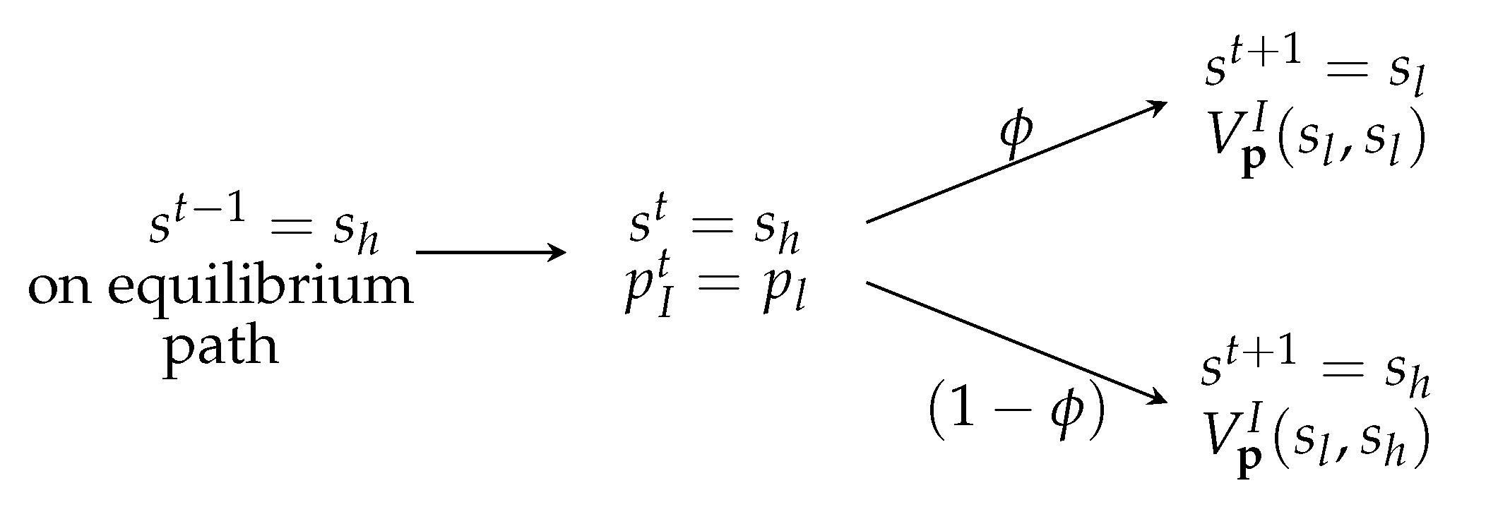
Next, we need to show that there are no profitable deviations from the price leadership profile. Firm can potentially make a profit by deviating to charge a lower price than the price prescribed by the strategy profile. Appendix A contains a detailed description of the potentially profitable deviations. All price cuts except one are immediately detected and therefore trigger a Nash reversal. Hence, price cuts that are immediately detected are not profitable for patient firms. The only price cut that is not detected occurs when both firms are supposed to set a price but firm I deviates by setting a price . In that case, the uninformed firm does not sell and cannot distinguish if there was a deviation or the state was . That deviation is depicted in Figure 1.
Figure 1 represents a situation in which firms have played according to the price leadership strategy profile up to period t and . Because the price of the informed firm was in the previous period, the uninformed sets a price at period t. Then, firm I can deviate by setting a price and getting the whole market instead instead of sharing the demand at price . Hence, the informed firm’s stage payoff from such deviation at period t is given by . The continuation values also change because the deviation leads to the uninformed firm setting a price at period . With probability the state at will change to and in that situation the informed firm faces an identical problem as when on equilibrium the state is going from to therefore obtaining a expected discounted payoff of . Similarly, with probability the state remains at period and the informed firm obtains a discounted payoff of .
Although high discount factors are enough to discourage all other price cuts in a price leadership profile, the firms being patient is not sufficient to discourage the informed firm from deviating according to Figure 1. Next we establish conditions to ensure that such deviation is not profitable. In the price leadership equilibrium, the informed firm does not set cut prices because doing so would lead the uninformed firm to match the lower price and to negatively impact the informed firm future profits.
3.2.1. Price Leadership Equilibrium with Monopolistic Prices
Next, I derive conditions that guarantee that price leadership with the monopolistic prices can be sustained as a PBE. All proofs are presented in Appendix B. Remember that an informed monopolist will set a price whenever the market size is low and a price if the market size is high. The next proposition establishes a condition on , and , so that price leadership with monopolistic prices is a PBE for patient enough firms.
Proposition 1.
If the following inequality holds,
there exists such that price leadership with monopolistic prices is a PBE for any .
In Figure 1, we presented a scenario in which the informed firm could deviate from the price leadership profile and increase its stage payoff without being detected. Whenever both firms set a high price , the uninformed firm could set a price . A feature of the proposed equilibrium is that the uninformed firm does not believe that the informed firm would deviate in such a way, and it does not monitor for such a deviation. For the informed firm, the cost of deviating is that the uninformed firm will follow and set a price in the next period. That is enough to deter the informed firm from deviating when condition (10) holds and firms are patient.
The condition (10) is intuitive given that the inequality holds for low and low . The informed does not want to deviate and set a price when both firms are supposed to set a price and split the high demand because:
- When is low, the monopolistic price for the low state, , is low relative to and that makes the option of deviating to set less desirable.
- When is low, the demand is persistent, the market size is likely to stay high in the next period and deviating would lead to a low price by the uninformed firm.
Furthermore, condition (10) is consistent with Stigler’s conjecture that “the prices of industries with price leaders are less flexible than those of industries without price leaders, despite the larger fluctuations of output of the former group.”3 Note that condition (10) implies that price leadership is more likely to arise if is low, a condition that generates more persistent prices. In a similar fashion, price leadership is more likely to arise if is not close to 1. As a result, changes are not small when price adjustments occur.
If the firms are able to sustain price leadership with monopolistic prices, joint profits are below the monopolistic profits only when there was a change of state and the the uninformed firm is not able to adjust its price. Therefore, as the market size becomes more persistent the joint profits must approximate monopolistic profits. The next lemma contains a closed form solution for the difference between the informed monopolist expected profits and the joint expected profits from following price leadership with monopolistic prices.
We compare the joint profits derived from price leadership with monopolistic prices to those obtained by an informed monopolist in the next lemma. The comparison will consider ex-ante profits, that is, before the informed firm or the informed monopolist know the realization of the current state.
Lemma 1.
The difference in ex-ante discounted payoffs between the informed monopolist and the joint profits of firms following price leadership with monopolistic prices are
and
where , the ex-ante expected payoff for the informed firm provided that the previous state was low, and similarly is its expected value when the previous state was high.
From Lemma 1, we conclude that the joint profits approach those of an informed monopolist as goes to 0. That is not necessarily the case when goes to 1 and everything else is fixed.
Proposition 2.
Fix and , then there exist a such that for any fixed ,
- Exists a , such that for any , price leadership with monopolistic profits is a PBE.
- The ex-ante expected joint profits go to the monopolistic profits as ϕ goes to 0.
The discount factor threshold, , is equal to when the ratio is below , and it is increasing on when the ratio is above .
Obara and Zincenko [13] show that is a necessary and sufficient condition for having a collusive outcome in an infinitely-repeated Bertrand duopoly with complete information.4 Therefore, in the limit case (when ), no collusion of any type could be possible when . Based on this result, we should expect that result to hold as approaches 0. In that case, if the ratio is sufficiently small and the shocks become sufficiently persistent, price leadership is an equilibrium whenever a collusive equilibrium is possible (more precisely, the discount factor threshold is the same as the minimum threshold in Obara and Zincenko [13]).
3.2.2. Price Leadership When Monopolistic Prices Are Not Sustainable
The results presented in Section 3.2.1 establish conditions under which firms are able to sustain monopolistic prices in a price leadership equilibrium. However, firms are able to sustain a price leadership equilibrium in cases in which monopolistic prices are not sustainable.
As previously argued, if patient firms cannot sustain monopolistic prices in a price leadership equilibrium, it must be the case that is too tempting for the informed firm to pretend that the demand is low when it is actually high. In such cases, a deviation like the one in Figure 1 can be discouraged by lowering the price assigned to the low demand state in the price leadership strategy profile. For example, it is easy to see that such a deviation is not profitable if . In general, for any , , and , a maximum can be derived such that price leadership with prices and is an equilibrium for patient firms.
4. Discussion
In this model, I study an infinite-horizon duopoly model in which firms engage in Bertrand competition at each period. The market size follows a two-state Markov process, and at each period the realization of the current state is only known by one firm. In that environment, I show the existence of equilibria that generates price leadership patterns for a wide set of parameters. Moreover, firms can derive joint profits that approach the monopolistic profits from this type of equilibria as the market size becomes more persistent. In such cases, given that overt communication is not feasible, the informed firm leads the uninformed firm towards joint profit maximization.
Moreover, compared to some previous models of barometric price leadership, we dispose of the assumption that firms have the option of pricing sequentially at each stage. We can understand pricing sequentially as a firm communicating their price intentions to competitors before making the price change, or as firms making non-immediately-effective price announcements as in the vitamins industry [14]. Our results suggest that firms can attain high profits through price leadership with no need for overt communication or price announcements.
Although our model differs from the “secret price cuts models”5 because firms are able to observe prices, the informed firm can cut prices without being detected by pretending that the demand is low when it is actually high. Price leadership discourages this type of deviation with no need for on-equilibrium punishments because if the informed firm lowers its price the uninformed will match the low price in the next period.
This paper provides theoretical support for Stigler’s barometric price leadership observations. The patterns can emerge in the presence of asymmetric information about persistent market conditions because the price of the better informed firm can be used to infer information about the unknown market conditions.
Funding
This research received no external funding.
Institutional Review Board Statement
Not applicable.
Informed Consent Statement
Not applicable.
Data Availability Statement
This study did not report any data.
Conflicts of Interest
The author declares no conflict of interest.
Appendix A. Potentially Profitable Deviations from Price Leadership
The potentially profitable deviations are listed below.
Lets start by analyzing the potential deviations by the uninformed firm.
- If the informed firm previous price was , the uninformed firm believes that the previous market size was and that the current state is with probability and with probability . Then, the uninformed firm can deviate by:
- -
- Charging a slightly lower price than . In that case, the uninformed firm gets the whole market and believes that with probability its stage payoff will be arbitrarily close to and with probability its stage payoff will be arbitrarily close to . This deviation triggers a Nash reversal. This type of deviation is not profitable if:
- -
- Charging a slightly lower price than (and above ). In that case, the uninformed firm sells only if the current state is , a scenario the uninformed firm believes to occur with probability and will lead to a stage payoff of . Again, this deviation triggers a Nash reversal and is not profitable as long as,
- Similarly, if the informed firm previous price was , the uninformed firm believes that the current state is with probability and with probability and can deviate by:
- -
- Charging a slightly lower price than . This type of deviation is not profitable as long as,
- -
- Charging a slightly lower price than . This type of deviation is not profitable if:
The potentially profitable deviations for the informed firm are listed next.
- When the demand goes from to : Because firms are following the price leadership profile, the informed firm previous price was implying that the uninformed firm current price is also . In this case, the only potentially profitable deviation is for the informed firm is to charge a price slightly below , a scenario in which the informed firm gets a stage payoff arbitrarily close to .This type of deviation is not profitable if:
- When the demand goes from to : The informed firm knows that the the uninformed is setting a price equal to so the only potentially profitable deviation is for the informed firm is to charge a price slightly below and get a stage payoff close to . This type of deviation is not profitable if:
- When the demand goes from to : In that case, the informed firm is obtaining the whole monopolistic profits in that period so there is no potential profitable deviation.
- When the demand goes from to : In that case, the uninformed sets a current price of because the informed previous price was . Then, there are two potential profitable deviations for the informed firm:
- -
- It can charge a price slightly below (and above ) and get a stage payoff close to . Such a deviation is not profitable as long as:
- -
- It can deviate by pretending the state is by charging a price as in Figure 1. The informed firm gets the whole market deriving a stage payoff of . The uninformed firm does not make a sale and therefore is not able to distinguish whether the market size was low or there was a deviation. Therefore, the next period the uninformed firm will set a price equal to . Furthermore, next period market size is with probability and the informed firm will face an identical problem as the case in which market size went from to . Similarly, next period market size is with probability and the informed firm will face an identical problem to the case in which the market size went from to . Consequently, if price leadership with monopolistic prices is an equilibrium, it must be the case that:
Appendix B. Proofs
We present proofs of the main results in this Appendix. We start by presenting close-form solutions for expected discounted payoffs when both firms are playing according to the price leadership strategy profile.
The following lemma will prove useful to calculate the values that firm derive from price leadership.
Lemma A1.
The solutions and to the system of equations
and
with , and are given by
Proof of Lemma A1.
Finally,
That completes the proof. □
Closed form solutions for the informed monopolist values and the informed firm calues can be derived using Lemma A1.
Corollary A1.
The expected ex-ante discounted payoff for an informed monopolist, solutions to the system of Equations (2) and (3), are given by
where and .
Corollary A2.
where and .
In a similar fashion we can obtain closed form solutions for the informed firm values.
Lemma A2.
The discounted expected values for the informed firm, , , and that are solutions to the system of Equations (6)–(9) are given by
where , , , and .
Proof of Lemma A2.
Again, let
and
Therefore, following exactly the same steps as in Lemma A1 we obtain
and
where and .
Note that Equation (6) is equal to,
Similarly, Equation (7) is equal to,
Next, Lemma A3 rewrites the incentive constraint (A8) in a way that not only simplifies the proof of Proposition 1 but also provides some intuition over the necessary conditions for the informed firm not to want to pretend that the demand is low when it is actually high.
Lemma A3.
The incentive constraint (A8) holds if and only if
Proof of Lemma A3.
The previous inequality can be rewritten as,
The last inequality can be written in the following way,
which completes the proof. □
Proof of Proposition 1.
Price leadership is a PBE as long as all the incentive constraints, (A1)–(A8), hold. Fix the prices to the respective monopolistic prices, that is, and . First note that the first seven incentive constraints, (A1)–(A7), correspond to price cutting deviations that are immediately detected. Therefore, any such deviation triggers a Nash reversal. As a result, any of those deviations is profitable if firms are patient enough because price leadership has a positive continuation value. Then, there exists a such that the incentive constraints (A1)–(A7) hold for any .
Now, it remains to show that the incentive constraint (A8) holds if firms are patient enough given the assumption (10). To do so, we start by plugging the monopolistic prices in Equation (A17).
Just plugging the profits,
or
Then, multiplying by , we can conclude that (A17) with monopolistic prices holds if and only if
where .
Denote the left-hand side of the previous inequality as the function f, that is, . The function f is continuous and differentiable in all arguments. Moreover, f is increasing on because
and decreasing on k whenever (10) holds since
Because f is continuous on , if (10) holds, there exists a such that for any , . Moreover, because f is increasing on ,
Proof of Lemma 1.
From Corollary A2,
where and .
Then, letting
and
From Corollary A1,
Therefore,
and
Furthermore,
and plugging the monopolistic prices,
Finally,
and
□
Proof of Proposition 2.
Fix and and let . We define
We will show that for any fixed , there exists a , such that for any price leadership with monopolistic prices is a PBE.
We fixed any . Now, given that we are fixing the discount factor, we must pay attention to those incentive constraints that correspond to deviations that trigger a Nash reversal. Therefore, we need to verify that all all the incentive constraints (A1)–(A8) are satisfied when goes to 0. First note that,
Next, we show that as goes to 0, the incentive constraint (A1) is satisfied as long as . Note that (A1) is satisfied if,
The left hand side of the previous inequality is continuous on for . Furthermore, when goes to 0, the left hand side goes to
Therefore, the incentive constraint (A1) holds when goes to 0 as long as . The same argument applies for incentive constraints (A2)–(A5) and (A7).
We are left with verifying that the incentive constraints (A6) and (A8) hold. Let us look at (A6), it holds if
When goes to 0, the left hand size of the previous inequality goes to
The previous expression can be written as
which is greater than 0 if
Therefore, the incentive constraint (A6) holds as goes to 0 as long as
Finally, using Lemma A3, we know that the incentive constraint (A8) holds as long as
and plugging the profits, that turns into,
If we multiply the previous inequality by , we would know that the inequality holds as
Note that the left hand side of the previous inequality is continuous on . Furthermore, as goes to 0, the left hand side goes to,
Consequently, the incentive constrain (A8) holds when goes to 0 as long as
Therefore, for any , there exists a , such that for any , price leadership with monopolistic prices is a PBE.
As a corollary of lemma 1, we can see that
This concludes the proof. □
| 1 | The model introduces information asymmetries into a two-firm and two-state version of Kandori [8]. |
| 2 | If the uninformed firm was unable to infer the state with certainty in any prior period, then the beliefs are derived in a similar manner from the initial distribution and the transition matrix. |
| 3 | See [1], on p. 446. |
| 4 | The described setting is a special case of Obara and Zincenko [13]. They consider a Bertrand oligopoly with complete information in which firms can have different discount factors. |
| 5 | See Section 6.7.1 in [15] for an example. |
References
- Stigler, G.J. The Kinky Oligopoly Demand Curve and Rigid Prices. J. Political Econ. 1947, 55, 432–449. [Google Scholar] [CrossRef]
- Markham, J.W. Nature and Significance of Price Leadership. Am. Econ. Rev. 1951, 41, 891–905. [Google Scholar]
- Rotemberg, J.J.; Saloner, G. Collusive Price Leadership; MIT Sloan Working Paper 2003-88; MIT Alfred P. Sloan School of Management: Cambridge, MA, USA, 1988. [Google Scholar]
- Cooper, D.J. Barometric price leadership. Int. J. Ind. Organ. 1997, 15, 301–325. [Google Scholar] [CrossRef]
- Rotemberg, J.J.; Saloner, G. Collusive Price Leadership. J. Ind. Econ. 1990, 39, 93–111. [Google Scholar] [CrossRef]
- Seaton, J.S.; Waterson, M. Identifying and characterising price leadership in British supermarkets. Int. J. Ind. Organ. 2013, 31, 392–403. [Google Scholar] [CrossRef] [Green Version]
- Escobar, J.F.; Llanes, G. Cooperation dynamics in repeated games of adverse selection. J. Econ. Theory 2018, 176, 408–443. [Google Scholar] [CrossRef]
- Kandori, M. Correlated Demand Shocks and Price Wars During Booms. Rev. Econ. Stud. 1991, 58, 171–180. [Google Scholar] [CrossRef]
- Deneckere, R.J.; Kovenock, D. Price Leadership. Rev. Econ. Stud. 1992, 59, 143–162. [Google Scholar] [CrossRef]
- Yano, M.; Komatsubara, T. Endogenous price leadership and technological differences. Int. J. Econ. Theory 2006, 2, 365–383. [Google Scholar] [CrossRef]
- Mouraviev, I.; Rey, P. Collusion and leadership. Int. J. Ind. Organ. 2011, 29, 705–717. [Google Scholar] [CrossRef]
- Yano, M.; Komatsubara, T. Price Competition or Tacit Collusion; KIER Discussion Paper 807; Kyoto University: Kyoto, Japan, 2012. [Google Scholar]
- Obara, I.; Zincenko, F. Collusion and heterogeneity of firms. RAND J. Econ. 2017, 48, 230–249. [Google Scholar] [CrossRef]
- Marshall, R.C.; Marx, L.M.; Raiff, M.E. Cartel price announcements: The vitamins industry. Int. J. Ind. Organ. 2008, 26, 762–802. [Google Scholar] [CrossRef]
- Tirole, J. The Theory of Industrial Organization; MIT Press: Cambridge, MA, USA, 1988. [Google Scholar]
Figure 1.
Undetected Deviation. In the cooperative phase of the price leadership profile, the informed firm can cut price without being detected.
Figure 1.
Undetected Deviation. In the cooperative phase of the price leadership profile, the informed firm can cut price without being detected.
Publisher’s Note: MDPI stays neutral with regard to jurisdictional claims in published maps and institutional affiliations. |
© 2021 by the author. Licensee MDPI, Basel, Switzerland. This article is an open access article distributed under the terms and conditions of the Creative Commons Attribution (CC BY) license (https://creativecommons.org/licenses/by/4.0/).
Share and Cite
MDPI and ACS Style
Gudino, G. Self-Enforcing Price Leadership. Games 2021, 12, 59. https://0-doi-org.brum.beds.ac.uk/10.3390/g12030059
AMA Style
Gudino G. Self-Enforcing Price Leadership. Games. 2021; 12(3):59. https://0-doi-org.brum.beds.ac.uk/10.3390/g12030059
Chicago/Turabian StyleGudino, Gustavo. 2021. "Self-Enforcing Price Leadership" Games 12, no. 3: 59. https://0-doi-org.brum.beds.ac.uk/10.3390/g12030059
Note that from the first issue of 2016, this journal uses article numbers instead of page numbers. See further details here.