Information Sharing in Oligopoly: Sharing Groups and Core-Periphery Architectures ^†

Abstract

The trade-off between the costs and benefits of disclosing a firm’s private information has been the object of a vast literature. The absence of incentives to share information on a common market demand prior to competition has been advocated to interpret information sharing as evidence of collusion. Recent contributions have looked at bilateral information sharing, showing that information sharing is consistent with pairwise stability, This paper studies the networked pattern of bilateral information sharing on market demand, focusing on the role of heterogeneous information (firms’ signals have different variances). We show that while pairwise stability predicts that i.i.d. signals are always shared in groups with a symmetric internal structure (both with and without side-payment and linking costs), heterogeneous signals are shared in asymmetric core-periphery architectures, in which “core” firms have more valuable information than periphery firms.

1. Introduction

In the recent economics literature, networks have been usefully employed to describe the patterns of communication and of diffusion of information among socio-economic agents. In the “connection model”, introduced in the seminal paper by Jackson and Wolinsky [1], agents benefit from the information disclosed by their neighbours and, with decreasing intensity, by the neighbours of their neighbours and so on. This model focuses on the benefits that the receiver of information enjoys. However in many economic applications agents may incur a cost from the disclosure of their own private information. When this is the case, the incentives to exchange information finally depend on the trade-off between these costs and the advantage of receiving new pieces of information in return.

This delicate trade-off has been studied in great detail by the literature on information sharing in oligopolistic markets. In one of the seminal papers of this literature, Vives [2] has shown that Cournot duopolists have no incentive to share private information before competing in quantities, unless they produce highly differentiated products. Other seminal papers have obtained results in the same spirit for markets with more than two firms (see, among others [3,4,5,6] and, more recently, [7]) In terms of economic policy, the absence of incentives to share information prior to competition directly implies that any evidence of information sharing should be interpreted as evidence of collusion, with obvious implication for social welfare (see, for instance, Kuhn and Vives [8] assessment of the EU industry).

All these papers assume that information is disclosed by firms to a centralised agency (e.g., a trade association), which then processes the information and transmits it back to firms.1 Recently, Currarini and Feri [9] have studied information sharing when players make binding exclusive bilateral agreements. In this setting, an information structure is well represented as an undirected network, whose nodes are the players that share information, and whose links are the bilateral sharing agreements. Their analysis applies to general linear quadratic games, and allows for both strategic complements and substitutes. For the specific case of Cournot oligopoly with demand uncertainty, it shows that the conditional correlation of signals may provide Cournot firms with incentives to share information even when products are perfectly homogeneous.

In the present paper we focus on the case of oligopolistic firms with private information on a demand parameter. Oligopolistic markets provide a setting where the networked structure of information is particularly relevant, since firms’ executives can accomplish sharing agreements in informal regular meetings, telephone calls, emails and so on, regardless of firms’ membership in a trade association. As in all papers prior to [9] we assume that signals are conditionally independent, but we allow firms to have heterogeneous information, here modelled in terms of different degree of informativeness of firms’ signals. The research question is how this heterogeneity affects the way in which information is shared and exchanged, that is, the architecture of the information sharing network.

We model market competition by means of a simplified version of the oligopolistic model studied by Gal-Or [6], in which each firm privately observes a piece of a linear demand curve (we further assume that firms observe signals without noise). Before getting to know their private signal, firms can engage in voluntary bilateral arrangements, by which they agree to (truthfully) share their own private information.2

We study the architecture of “pairwise stable” networks (see [1]), that is networks in which no pair of firms would agree to make a new sharing arrangement, and in which no firm wishes to unilaterally discontinue an existing one.3 Although somewhat specific, the additive structure of information we employ allows us to study the case of unconditionally independent signals (a case ruled out under the usual assumption that firms receive a signal form the same prior distribution of a single demand parameter) for which we fully characterise the set of stable networks both for homogeneous and for heterogeneous signals.

More specifically, we find that when signals are i.i.d., information sharing is organised in fully connected components, that is “groups” of firms in which all members’ information becomes common knowledge.4 We also show that when side payments are possible between sharing firms, then only one sharing group forms, within which all information is shared. When information sharing involves an exogenous cost (time, coordination efforts, verification costs, monitoring,…), sharing groups have an incomplete, though regular, internal structure, and information does not become common knowledge within the group. In the case of heterogeneous signals we show that non regular architectures emerge. In particular, core-periphery networks are stable, in which firms with more valuable information are embedded in a densely connected core, while the other firms are located at the periphery of the network.

The paper is organised as follows: Section 2 describes the model. Section 3 contains all the results. Section 4 concludes the paper.

2. The Model

We consider a n-firms oligopolistic market with linear demand and no costs. The size of the market, given by the intercept of the demand function, is the sum of n random variables $a_1, a_2, ..., a_n$ plus a deterministic part A:

$$p\left(Q\right)=A+a-bQ,$$

(1)

where $Q\equiv {\displaystyle \sum _{i=1}^n}{q}_i$ is the aggregate produced level in the market, and where $a\equiv a_1+a_2+...+a_n$. The random variables $\left(a_1, a_2, ..., a_n\right)$ are independently normally distributed with zero mean and variances ${\sigma }_{11}, {\sigma }_{22}, ...., {\sigma }_{nn}$.

Each firm i directly observes the random variable $a_i$. Moreover, and before the realisation of these private“signals”, firms can share their private information by means of bilateral contracts. More precisely, any pair of firms i and j can commit to truthfully exchange their private information, in which case firm i gets to observe the realisation of the random variable $a_j$ and vice versa. The information structure generated by a set of bilateral sharing contracts can be usefully described by a non directed network.

Given a set N, a non directed network g is defined as any subset of the set of all (unordered) pairs of elements in N:

$$g\subseteq \left\{ij:i\in N\mathrm{and}j\in N,i\ne j\right\}.$$

The elements of N are called nodes, and a pair $ij\in g$ is called a “link”. We denote by $N_i^g=\left\{j\in N:ij\in g\right\}\cup \left\{i\right\}$ the neighbourhood of i in g, with cardinality $n_i^g$ (this cardinality is called “degree” of i). We will denote by $g-ij$ the network obtained from g by deleting the link $ij\in g$ and by $g+ij$ the network obtained from g by adding the link $ij\notin g$.

The network g is connected if for all pairs i and j in N there exists a connecting path $P(i,j)$, that is, a set $\left\{i_1,i_2,...,i_k\right\}$ such that $i=i_1$, $j=i_k$, and $i_p{i}_{p+1}\in g$ for all $p=1, ..., k-1$.

Given the network g, the network h is a subnetwork of g if $h\subseteq g$; with abuse of notation we denote the set of nodes in h by $N_h:=\{i\in N:\{(i,1),...,(i,n)\}\cap h\ne \varnothing \}$. We say that h is a component of g if it is connected and if for all $i\in N_h$ and $j\notin N_h$ we have $ij\notin g$. The size of a component h is denoted by $n\left(h\right)$, that is, the cardinality of the set $N_h$. A component h is: (i) regular if $n_i^g=n_j^g$$\forall i,j\in N_h$, that is, all nodes in $N_h$ have the same degree, in this case we call $n_i^g$ the degree of the component, (ii) completely connected if $n\left(h\right)=$$n_i^g=\forall i\in N_h$, that is, it is regular and its size coincides with its degree.

With some abuse of terminology, we will say that the network g is regular when all its components are regular.

2.1. The Bayesian Cournot Game for a Given Network

After the realisation of the random variables $a_1,a_2,...,a_n$ firms play the Cournot game with incomplete information ${\mathsf{\Gamma }}^g$, in which the information available to firm i is given by the set of signals it observes, that we denote by $a_i^g$. The ex-ante expected profits in such game will determine the incentives of firms to make information sharing arrangements (see next subsection).

A pure strategy for firm i is a function $s_i:R_{+}^{n_i^g}\to R_{+}$ setting a quantity level for each possible vector of signals observed by i. Let $E\left[{\pi }_i(s_1,s_2,...,s_n)|a_i^g\right]$ denote the expected profit of firm i in g given $a_i^g$ and given that quantities are fixed according to the strategy profiles $(s_1,s_2,...,s_n)$. A Bayesian Nash equilibrium of this game ${\mathsf{\Gamma }}^g$ is a profile of strategies ${\left(s_i^{*}\right)}_{i=1,...,n}$ such that for all i, for all $q_i$ and for all $a_i^g:$

$$E\left[{\pi }_i(s_i^{*},s_{-i}^{*})|a_i^g\right]\ge E\left[{\pi }_i(q_i,s_{-i}^{*})|a_i^g\right].$$

2.2. The Link Formation Stage

Firms arrange sharing contracts before they actually observe their own signals, and anticipate the equilibrium outcome in the Cournot game. Incentives to share information are therefore defined in terms of ex-ante expected profits in alternative networks. We will denote by $E_i^g$ the expectation of firm i taken over all possible realizations of $a_i^g$; moreover, to keep notation simple, we denote by ${\pi }_i\left(a_i^g\right)$ the expected equilibrium profit $E\left[{\pi }_i(s_i^{*},s_{-i}^{*})|a_i^g\right]$ of firm i in ${\mathsf{\Gamma }}^g$ given $a_i^g$.

The notion of pairwise stable network, first introduced in [1], provides a minimal notion of stability in the link formation process, requiring that no link is added or severed from a stable network.

Definition 1.

The network g is pairwise stable iff:

$$\begin{array}{cc}\hfill E_i^g\left[{\pi }_i\left(a_i^g\right)\right]{-E}_i^g\left[{\pi }_i\left(a_i^{g-ij}\right)\right]& \ge 0\mathit{and}{E}_j^g\left[{\pi }_j\left(a_j^g\right)\right]{-E}_j^g\left[{\pi }_j\left(a_j^{g-ij}\right)\right]\ge 0\forall ij\in g;\hfill \end{array}$$

(2)

$$\begin{array}{cc}\hfill \mathrm{if}{E}_i^g\left[{\pi }_i\left(a_i^{g+ij}\right)\right]{-E}_i^g\left[{\pi }_i\left(a_i^g\right)\right]& >0\mathit{then}{E}_j^g\left[{\pi }_j\left(a_j^{g+ij}\right)\right]{-E}_j^g\left[{\pi }_j\left(a_j^g\right)\right]<0\forall ij\notin g.\hfill \end{array}$$

(3)

A stronger notion of stability allows each firm to revise any subset of its links (instead of only one link), and any pair of firms to form a new one. This notion of pairwise Nash stability has been sometimes used in the literature (see [12]). We will primarily be concerned with the notion of pairwise stability, which most stresses the bilateral nature of our analysis.5

3. Results

In this section we present the main results starting with how firms use information in a given network. Then we study information sharing first in the case of homogeneous signals (with and without side payments and linking costs) and then we move to the case of heterogeneous signals that allow more complex equilibrium architectures.

3.1. Bayesian Cournot Equilibrium for a Given Network

By standard results on linear Cournot games with incomplete information (see Radner (1962)), equilibrium strategies are affine in signals, that is:

$$s_i\left(a_i^g\right)={\alpha }_i+{\sum }_{j\in N_i^g}{\beta }_{ij}{a}_j,$$

(4)

where ${\alpha }_i$ is the constant term of the equilibrium strategy of firm i, and by ${\beta }_{ij}$ the coefficient applied by firm i to each element $a_j$ of the vector $a_i^g$.

Proposition 1.

Equilibrium parameters are defined by the following set of equations:

$$\begin{array}{c}{\beta }_{ij}=\frac{1-b{\displaystyle \sum _{h\in N_j^g\setminus \left\{i\right\}}}{\beta }_{hj}}{2b},\forall j\in N_i^g\end{array}$$

(5)

$$\begin{array}{c}{\alpha }_i=\frac{A-b{\sum }_{h\ne i}{\alpha }_h}{2b}.\end{array}$$

(6)

The proof this and all other results of the paper can be found in the Appendix A. We first note that the $\alpha$ parameters are defined by an independent set of equations, and that they do not depend on the network g. Since the expected values of all signals is zero, this implies that the expected aggregate quantity is the same in each network.

We then observe that the expression for the terms $\beta$ has intuitive interpretations that highlight the role of the network in shaping equilibrium behaviour. The term ${\beta }_{ij}$ (measuring the reaction of firm i to the observed signal $a_j$) is determined by the use that firm i makes of signal $a_j$ to estimate the intercept minus a term that measures the use that other firms make of signal $a_j$, that is, firm i reacts less to signal $a_j$ the more numerous are the firms that observe $a_j$ and base their decisions on it. Intuitively, the information provided by signal $a_j$ is more valuable the less it is observed by other firms—a clear congestion effect on which we will return in the next sections. From (5) we note that for each j, the equilibrium coefficients applied to signal $a_j$ by the firms in $N_j^g$ are determined by an independent set of identical equations, so that ${\beta }_{ij}={\beta }_{hj}$ for all i and h in $N_j^g$. From (6) ${\alpha }_i={\alpha }_h$ for all $i,h\in N$. These considerations are summarised in the following corollary.

Corollary 1.

Equilibrium parameters are:

$$\begin{array}{c}{\beta }_{ij}=\frac{1}{b(n_j^g-1)},\forall i\in Nand\forall j\in N_i^g\end{array}$$

(7)

$$\begin{array}{c}{\alpha }_i=\frac{A}{b(n+1)},\forall i\in N.\end{array}$$

(8)

We finally determine expected equilibrium profits in ${\mathsf{\Gamma }}^g$. The following result relates the expected profits of a firm to its equilibrium quantity (see Proposition 1 in [14]).

Lemma 1.

Ex-ante expected profits of firm i in the game ${\mathsf{\Gamma }}^g$ are given by:

$$E_i^g\left[{\pi }_i\left(a_i^g\right)\right]=b{E}_i^g\left[s_i^{*}{\left(a_i^g\right)}^2\right].$$

Since $s_i^{*}{\left(a_i^g\right)}^2$ is a square of a linear function in $a_i^g$ (i.e., Equation (4)), using the assumption of signals independence and Corollary 1, it follows that ex-ante profits are given by a constant term plus a term that is proportional to the variance of the equilibrium quantities.

Corollary 2.

Ex-ante profits are of firm i in the game ${\mathsf{\Gamma }}^g$ are given by:

$$\begin{array}{c}{E}_i^g\left[{\pi }_i\left(a_i^g\right)\right]=\frac{A^2}{b{(n+1)}^2}+{\sum }_{j\in N_i^g}\frac{{\sigma }_{jj}}{b{(n_j^g-1)}^2}.\end{array}$$

(9)

Note that the summatory represents the variance of the equilibrium quantities multiplied by parameter b. Therefore the ex-ante profits of firm i are increasing with the variability of its strategy. It directly follows that the difference in ex-ante profits in two different networks is measured by the difference in the variance of equilibrium quantities.

3.2. Information Sharing When Signals Are Homogeneous

Here we assume that signals have the same variance. For this case the next proposition states necessary and sufficient conditions for a network to be pairwise stable.

Proposition 2.

A network g is pairwise stable if and only if both of the following conditions are verified.

For all $ij\in g$

$$\begin{array}{c}\frac{1}{{(n_j^g+1)}^2}\ge \frac{1}{{\left(n_i^g\right)}^2}-\frac{1}{{(n_i^g+1)}^2};\end{array}$$

(10)

$$\begin{array}{c}\frac{1}{{(n_i^g+1)}^2}\ge \frac{1}{{\left(n_j^g\right)}^2}-\frac{1}{{(n_j^g+1)}^2}.\end{array}$$

(11)

For all $ij\notin g$:

$$\begin{array}{c}\frac{1}{{(2+n_j^g)}^2}>\frac{1}{{(1+n_i^g)}^2}-\frac{1}{{(2+n_i^g)}^2}\end{array}$$

(12)

$$\begin{array}{c}\mathit{implies}\frac{1}{{(2+n_i^g)}^2}<\frac{1}{{(1+n_j^g)}^2}-\frac{1}{{(2+n_j^g)}^2}.\end{array}$$

(13)

The intuition behind conditions (10)–(13) can be explained as follows. Conditions (10) and (11) require that no link in a stable network is severed. On the LHS of (10) is the loss to firm i from severing the link $ij$ in terms of i’s equilibrium quantity’s variance; this is measured by the variability of firms i’s strategy with respect to signal $a_j$ (see Lemma 1), normalised by the number of firms that see signal $a_j$ (the larger this number, the less valuable is signal $a_j$). This loss in expected profits has to be larger than the gain from severing link $ij$ (RHS); this is measured as the increase in the “value” of signal $a_i$, which in case of severance of link $ij$ is observed by one less firm. Condition (11) requires the same for j. Conditions (12) and (13) requires that no link is added to a stable network. On the LHS of (12) is the gain to firm i from forming the new link in terms of the variability of firm i’s strategy with respect to the newly acquired signal $a_j$; on the RHS is the net loss in variability due to the fact that one additional firm (firm j) observes signal $a_i$. If the LHS exceeds the RHS for firm i, then the reverse must hold for firm j (condition (13)).

Note that the incentives to form or sever link $ij$ only depend on the degrees of the nodes i and j, and on no other features of the network. In particular, the gain in profit due to a link with node j decreases with the degree of j. It is indeed possible to determine two thresholds in the degree of a node j: the value $F\left(n_i\right)$ above which a node i of degree $n_i$ would not maintain the link $ij,$ that is, if $n_j>F\left(n_i\right)$ condition (10) is not satisfied; the value $f\left(n_i\right)$ above which a node i of degree $n_i$ would not form the new link $ij$; that is, if $n_j>f\left(n_i\right)$ inequality (12) is not satisfied. These thresholds are formally defined in Lemma A1 in the Appendix A, where we show, together with other properties, that both F and f are increasing in $n_i$, meaning that the incentives of node i to link with a given node j increase with the degree of i.

The next proposition fully characterises the set of pairwise stable networks for the case of i.i.d. signals.

Proposition 3.

Let $n\ge 3$. The set of pairwise stable networks contains: the empty network, the complete network, and all networks made of $s\le n-3$ isolated nodes and $p\ge 1$ completely connected components of size $n_1\ge 3,n_2,...,n_p$ such that $n_i>f\left(n_{i-1}\right)$ for all $i=2,...,p$.

The set of pairwise stable networks characterised in Proposition 3 is very large. However, Proposition 3 provides two precise qualitative predictions on how information is shared in equilibrium. First, information sharing is essentially organised in groups (the completely connected components), within which the transmission of information is equivalent to one in which firms publicly disclose their signal to all other firms in the group. This type of public disclosure characterises all previous works on the subject, and is here obtained endogenously as a result of private and bilateral arrangements. Second, information sharing groups must be of different size, to make sure that firms in different groups do not form links (in fact, from point 3.d in Lemma A1 in the Appendix A, firms with similar degree link together).

Now we study two extensions: in the first we allows for side-payments, in the second we impose an exogenous link cost.

3.2.1. Side-Payments

The above definition of pairwise stability implicitly rules out the possibility of side payments between firms which are contingent on the sharing of information. In the presence of such transfers, conditions (2) and (3) would be replaced by the following condition (see [1]):

$$\begin{array}{cc}\hfill E_i^g\left[{\pi }_i\left(a_i^g\right)\right]+E_j^g\left[{\pi }_j\left(a_j^g\right)\right]-E_i^g\left[{\pi }_i\left(a_i^{g-ij}\right)\right]-E_j^g\left[{\pi }_j\left(a_j^{g-ij}\right)\right]& \ge 0\forall ij\in g;\hfill \end{array}$$

(14)

$$\begin{array}{cc}\hfill E_i^g\left[{\pi }_i\left(a_i^{g+ij}\right)\right]+E_j^g\left[{\pi }_j\left(a_j^{g+ij}\right)\right]-E_i^g\left[{\pi }_i\left(a_i^g\right)\right]-E_j^g\left[{\pi }_j\left(a_j^g\right)\right]& \le 0\forall ij\notin g.\hfill \end{array}$$

(15)

We obtain a more narrow prediction for the case in which firms can agree on side-payments which are contingent on information sharing. In this case, the formation of links that bridge two components is made easier by the sharing of individual gains, and at most one component of information sharing firms can be compatible with stability.

Proposition 4.

When side payments are possible, the set of pairwise stable networks contains: the empty network, the complete network, all networks g made of one completely connected component h of size $n\left(h\right)\ge 3$ and $n-n\left(h\right)$ isolated nodes.

So far, all stable structures that differ from the empty network only admitted fully connected components.

3.2.2. Costly Links

Now we study the case in which the formation of a link has a fixed and exogenous cost c, representing all monetary expenditures that a firm bears in order to arrange and execute an information sharing arrangement. Interestingly, in this new setting both market conditions (the slope b of the demand function) and the variance $\sigma$ of signals turn out to play a role in shaping the incentives of firms to form and sever links. The following new stability conditions are obtained by a minor modification of the proof of Proposition 2: for all $ij\in g$:

$$\begin{array}{cc}\hfill \frac{1}{{(n_j^g+1)}^2}+\frac{1}{{(n_i^g+1)}^2}-\frac{1}{{\left(n_i^g\right)}^2}& \ge \frac{b^{2}c}{\sigma }\hfill \end{array}$$

(16)

$$\begin{array}{cc}\hfill \frac{1}{{(n_i^g+1)}^2}+\frac{1}{{(n_j^g+1)}^2}-\frac{1}{{\left(n_j^g\right)}^2}& \ge \frac{b^{2}c}{\sigma }.\hfill \end{array}$$

(17)

For all $ij\notin g$:

$$\begin{array}{ccc}\hfill \frac{1}{{(2+n_i^g)}^2}+\frac{1}{{(2+n_j^g)}^2}-\frac{1}{{(1+n_i^g)}^2}& >& \frac{b^{2}c}{\sigma }\hfill \end{array}$$

(18)

$$\begin{array}{ccc}\hfill \mathrm{implies}\frac{1}{{(2+n_j^g)}^2}+\frac{1}{{(2+n_i^g)}^2}-\frac{1}{{(1+n_j^g)}^2}& <& \frac{b^{2}c}{\sigma }.\hfill \end{array}$$

(19)

A more elastic demand (small b) provides higher incentives to maintain (and to form) links (this is in line with the intuition that more competitive markets, and therefore a lower strategic interdependence of firms, facilitate information sharing—see [15]). These incentives also increase with the variance $\sigma$, which has the effect of scaling up the informational gain of new connections. It will be convenient to refer to the gross cost parameter $C={\displaystyle \frac{b^{2}c}{\sigma }}$, and refer to the single elements of C only when these provide interesting economic insights.

An interesting question is whether incomplete and stable components can emerge, and, in this case, of which size. For all $c\ge 0$, let $f_C\left(n_i\right)$ be the value above which a node i of degree $n_i$ would not form the new link $ij$; that is, if $n_j>f_C\left(n_i\right)$ condition (18) is not satisfied; and let $m_1\left(C\right)$($m_2\left(C\right))$ be the first integer above (below) the smaller (larger) solution of $\left(\frac{2}{{(m+1)}^2}-\frac{1}{{\left(m\right)}^2}\right)\ge C$. With this notation we can state the following proposition.

Proposition 5.

Let $c>0$, then the set of pairwise stable networks contains the empty network and all networks made of $s\le n-m_1\left(C\right)$ isolated nodes and $p\ge 1$ regular components h with $n\left(h\right)>m_1\left(C\right)$. Components h with $n\left(h\right)>m_1\left(C\right)$ have the following characteristics: (i) if $n\left(h\right)\le m_2\left(C\right)$ are fully connected, otherwise have degree equal to $m_2\left(C\right)$; (ii) each pair of components h, $h^{\prime }$ with $n\left(h\right)\le n\left(h^{\prime }\right)<m_2\left(C\right)$ satisfies $n\left(h^{\prime }\right)>f_C\left(n\left(h\right)\right)$.

Proposition 5 basically sets the upper bound $m_2\left(C\right)$ on the degree of a stable completely connected component. Although one may be tempted to understand this as a consequence of the large aggregate cost paid in completely connected components of large size, this is not the case. Indeed, here the decision to sever or maintain a given link only depends on the comparison between the change in payoffs and the marginal cost c. What drives the existence of the upper bound $m_2\left(C\right)$ is, instead, the fact that the incentives to maintain a link are decreasing in the degree of the nodes, and larger components fail to be stable as a result. There is therefore an inverse relation between the density of a component (ratio between average degree and size) and its size.

3.3. Sharing Heterogeneous Signals in Core-Periphery Networks

In this section we relax the assumption that signals are identically distributed, and allow the variances of signals (i.e., the parameters $a_i$) to differ across firms. The stability conditions of Proposition 2 are modified to account for this new source of heterogeneity: the network g is pairwise stable if and only if:

-

for all $ij\in g$:

$$\begin{array}{cc}\hfill \frac{{\sigma }_{jj}}{{(n_j^g+1)}^2}& \ge \frac{{\sigma }_{ii}}{{\left(n_i^g\right)}^2}-\frac{{\sigma }_{ii}}{{(n_i^g+1)}^2}\hfill \end{array}$$

(20)

$$\begin{array}{cc}\hfill \frac{{\sigma }_{ii}}{{(n_i^g+1)}^2}& \ge \frac{{\sigma }_{jj}}{{\left(n_j^g\right)}^2}-\frac{{\sigma }_{jj}}{{(n_j^g+1)}^2},\hfill \end{array}$$

(21)

-

for all $ij\notin g$:

$$\begin{array}{cc}\hfill \frac{{\sigma }_{jj}}{{(2+n_j^g)}^2}& >\frac{{\sigma }_{ii}}{{(1+n_i^g)}^2}-\frac{{\sigma }_{ii}}{{(2+n_i^g)}^2}\hfill \end{array}$$

(22)

$$\begin{array}{cc}\hfill \mathrm{implies}\frac{{\sigma }_{ii}}{{(2+n_i^g)}^2}& <\frac{{\sigma }_{jj}}{{(1+n_j^g)}^2}-\frac{{\sigma }_{jj}}{{(2+n_j^g)}^2}.\hfill \end{array}$$

(23)

We see that, given the degrees $n_i^g$ and $n_j^g$, the incentive of i to sever the link $ij$ increases with the ratio of variances ${\displaystyle \frac{{\sigma }_{ii}}{{\sigma }_{jj}}}$ (conditions (20) and (21)) and the incentive of i to form the link $ij$ decreases with ${\displaystyle \frac{{\sigma }_{ii}}{{\sigma }_{jj}}}$ (condition (22)). This effect can be understood in terms of the additional variability of i’s equilibrium quantity coming from the link $ij$. The higher the term ${\sigma }_{jj}$, the higher the additional variability of i’s quantity due to the link $ij$, and the higher the informational “ value” of j’s signal for firm i. Similarly, the higher the term ${\sigma }_{ii}$, the lower the incentive of firm i to form the link $ij$; this because it is more costly to share a signal with higher variance with one additional firm. Again, a high value of ${\sigma }_{ii}$ reflects therefore a high informational value of i’s signal.

Note that in this setting of heterogeneous variance, a firm with high variance may not wish to maintain a link (or to form a new one) with another firm with same degree but lower variance. As a consequence, while the empty network is always a pairwise stable information structure (as was proved for the case of i.i.d. signals), the complete network may fail to be stable when firms have significant heterogeneity in variances. However, as the next proposition shows, this can only happen when the number of firms is small.

Proposition 6.

(1) The empty network is pairwise stable for all distributions of variances, even if side payments are possible; (2) There exist configurations of variances for which the complete network is not pairwise stable; (3) For every configuration of variances, there exists a finite number of firms $\overline{n}$ such that for all $n\ge \overline{n}$ the complete network is pairwise stable.

While we refer to the Appendix A for details, the intuition of this result is clear: when the degree of two nodes increases, their difference in variances becomes less and less relevant in the stability conditions (20) and (21).

We next turn to the existence of pairwise stable networks with non completely connected components. Since signals with large variance possess higher informational value, the incentive to link to firms observing such signals may remain high even when these firms have a large degree. We can therefore envisage stable architectures in which firms with large variance have larger degree than firms with low variance. We show that a special class of incomplete architectures, usually referred to as “core-periphery networks”, can be pairwise stable for suitable distributions of variances. In more detail, core periphery networks present a dense set of interconnected nodes—the core—each linked with all nodes in the network, and sets of peripheral nodes which are internally connected and are linked with the core nodes. Formally, a core-periphery network g consists of a set $\left\{g_1,g_2,....g_H\right\}$ of fully connected subnetworks, such that $i\in g_k$ and $j\in g_m$ implies that $ij\notin g$ for all $k\ne m$ such that $k\in \left\{2,3,...,H\right\}$ and $m\in \left\{2,3,...,H\right\}$, and such that $i\in g_1$ and $j\in g_k$ implies $ij\in g$ for all $k=1,2,3,...,H$. We call the subnetwork $g_1$core (with size $n_c$), and the subnetworks $\left\{g_2,....g_H\right\}$ peripheries. We define a symmetric core-periphery network as one in which all peripheral firms have the same size $n_p\ge 1$. We also say that peripheries are consecutive in variances if they can be obtained as a consecutive partition of the set of peripheral nodes ordered with respect to variance.

Proposition 7 provides two qualitative features of pairwise stable symmetric core-periphery networks: peripheral firms are organised in groups that are consecutive in variance, and core firms have larger variance than peripheral firms.

Proposition 7.

Every symmetric pairwise stable core periphery network is such that peripheries are consecutive in variances. Moreover, for each given size $n_p$, there exists a finite $n^{\prime }$ such that if $n>n^{\prime }$ then every symmetric pairwise stable core periphery network is such that ${min}_{i\in g_1}{\sigma }_i>{max}_{j\in g\setminus g_1}{\sigma }_j$.

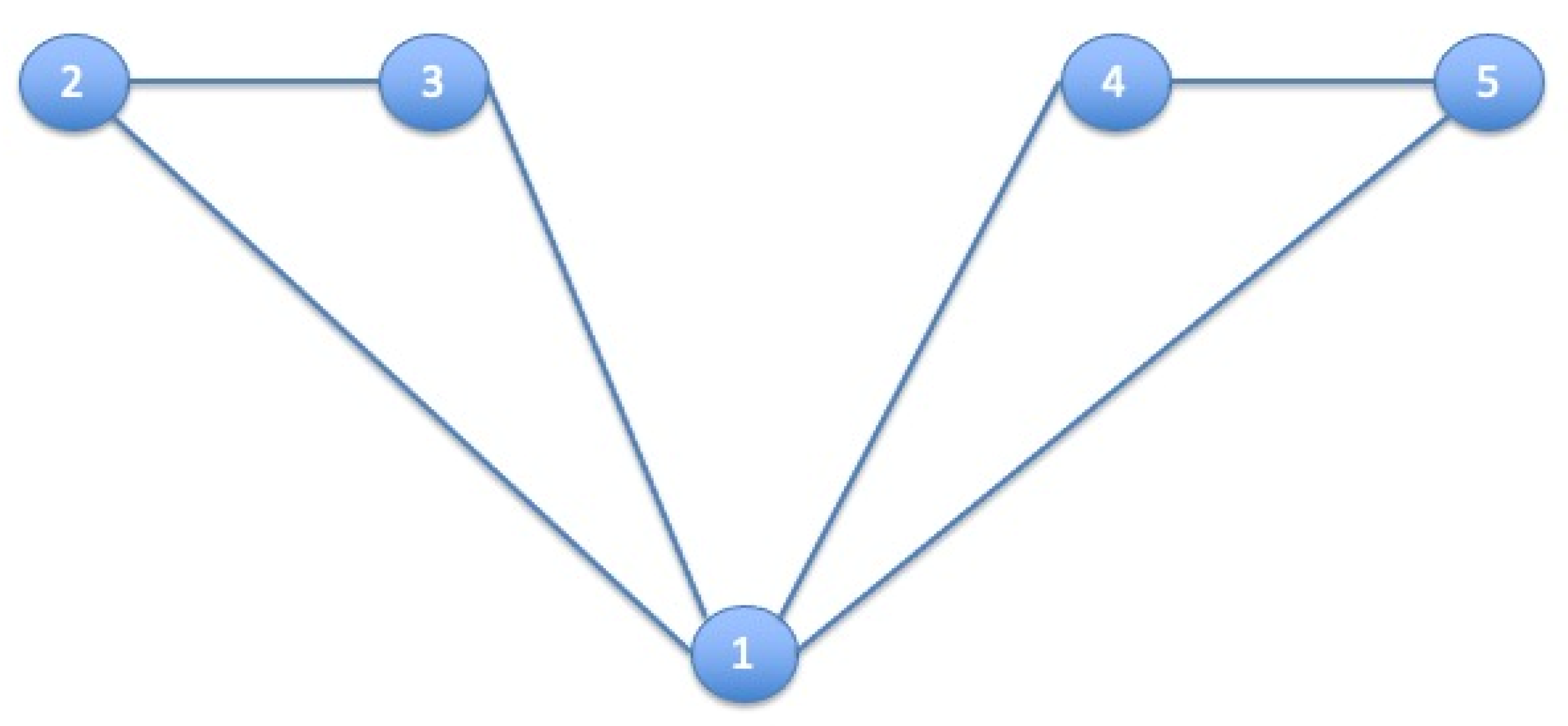
Intuitively, core firms observe signals that are publicly observed, and have therefore lower informational value. These signals are more“desirable” the larger their variance, from which the second result in Proposition 7. An example of pairwise stable core periphery network is the following (see Figure 1).

Example 1.

Consider a network with 5 nodes: node 1 is the “core” node, while the two peripheries are $\left\{23\right\}$ and $\left\{45\right\}$. Variances are ${\sigma }_1=1$, ${\sigma }_2={\sigma }_3=\frac{1}{5}$, ${\sigma }_4={\sigma }_5=\frac{1}{2}$. Relevant stability conditions (20)–(23) (for links 12, 15 and 34, respectively) are satisfied:

$$\frac{1}{36}+\frac{1}{5}\frac{1}{16}\ge \frac{1}{25};\frac{1}{36}+\frac{1}{2}\frac{1}{16}\ge \frac{1}{25};\left(\frac{1}{2}+\frac{1}{5}\right)\frac{1}{25}\le \frac{1}{5}\frac{1}{36}.$$

4. Concluding Remarks

We have studied the incentives of oligopolistic firms to share information on a random demand intercept by means of bilateral contracts. We have assumed that sharing agreements are bilateral, and that firms can revise one sharing agreement at a time. Our results have shown that when the cost of implementing a sharing agreement are not too high and information is symmetric, then sharing occurs in groups or coalitions, within which information is universally disclosed. When costs are high, information is shared “locally” within groups, with each firm disclosing only to a subset of other group members. When information is heterogeneous, then asymmetric sharing architectures arise, where core firms (with less informative signals) share more intensely than periphery firms.

All of our analysis has made the assumption that signals are shared at the ex-ante stage, before private information is revealed to firms. An interesting alternative approach would allow firms to share information at the interim stage, and explore the rich strategic structure of an interim model of information sharing. One possible conjecture would be that in this case the complete network could emerge as the unique stable structure. In a nutshell, the mechanism would go as follows. Given that firms have an incentive to hide good signals and to reveal bad signals, one could suppose that firms adopt a threshold strategy, hiding their private information when it is good (the signal is greater than a given level) and revealing it when it is bad (below that level). Differently from the ex-ante stage, here the disclosure decision is itself informative: when a firm does not reveal, it implicitly signals to possess good information. This would trigger an update of the competitors’ priors upwards. In turns, this update would move the thresholds in the disclosure strategy upwards and, by successive iterations, the threshold would reach the maximum admissible value of the signal, with the total unraveling of information. We leave this important issue for future research.

References

- Jackson, M.O.; Wolinsky, A. A strategic model of social and economic networks. J. Econ. Theory 1996, 71, 44–74. [Google Scholar] [CrossRef]
- Vives, X. Duopoly Information Equilibrium: Cournot and Bertrand. J. Econ. Theory 1985, 34, 71–94. [Google Scholar] [CrossRef]
- Novshek, W.; Sonnenschein, H. Fulfilled expectations Cournot duopoly with information acquisition and release. Bell J. Econ. 1982, 13, 214–218. [Google Scholar] [CrossRef]
- Clarke, R. Collusion and the Incentives for Information Sharing. Bell J. Econ. 1983, 14, 383–394. [Google Scholar] [CrossRef]
- Li, L. Cournot oligopoly with information sharing. Rand J. Econom. 1985, 16, 521–536. [Google Scholar] [CrossRef] [Green Version]
- Gal-Or, E. Information Sharing in Oligopoly. Econometrica 1985, 53, 329–343. [Google Scholar] [CrossRef]
- Raith, M. A General Model of Information Sharing in Oligopoly. J. Econ. Theory 1996, 71, 260–288. [Google Scholar] [CrossRef] [Green Version]
- Kühn, K.U.; Vives, X. Information Exchanges among Firms and their Impact on Competition; Office for Official Publications for the European Community: Luxemburg, 1995. [Google Scholar]
- Currarini, S.; Feri, F. Information Sharing Networks in Linear Quadratic Games. Int. J. Game Theory 2015, 44, 701–732. [Google Scholar] [CrossRef]
- Ziv, A. Information Sharing in Oligopoly: The Truth Telling Problem. Rand J. Econ. 1993, 24, 455–465. [Google Scholar] [CrossRef]
- Doyle, M.P.; Snyder, C.M. Information Sharing and Competition in the Motor Vehicle Industry. J. Political Econ. 1999, 107, 1326–1364. [Google Scholar] [CrossRef] [Green Version]
- Bloch, F.; Jackson, M.O. Definitions of Equilibrium in Network Formation Games. Int. J. Game Theory 2006, 34, 305–318. [Google Scholar] [CrossRef]
- Jackson, M.O.; van den Nouweland, A. Strongly Stable Networks. Games Econ. Behav. 2005, 51, 420–444. [Google Scholar] [CrossRef] [Green Version]
- Kirby, A.J. Trade Associations as Information Exchange Mechanisms. Rand J. Econom. 1988, 19, 138–146. [Google Scholar] [CrossRef]
- Vives, X. Trade Association Disclosure Rules, Incentives to Share Information and Welfare. Rand J. Econ. 1990, 21, 409–430. [Google Scholar] [CrossRef]
Figure 1.
Core-Periphery Network with five nodes.
Publisher’s Note: MDPI stays neutral with regard to jurisdictional claims in published maps and institutional affiliations. |
© 2021 by the authors. Licensee MDPI, Basel, Switzerland. This article is an open access article distributed under the terms and conditions of the Creative Commons Attribution (CC BY) license (https://creativecommons.org/licenses/by/4.0/).
Share and Cite
MDPI and ACS Style
Currarini, S.; Feri, F. Information Sharing in Oligopoly: Sharing Groups and Core-Periphery Architectures. Games 2021, 12, 95. https://0-doi-org.brum.beds.ac.uk/10.3390/g12040095
AMA Style
Currarini S, Feri F. Information Sharing in Oligopoly: Sharing Groups and Core-Periphery Architectures. Games. 2021; 12(4):95. https://0-doi-org.brum.beds.ac.uk/10.3390/g12040095
Chicago/Turabian StyleCurrarini, Sergio, and Francesco Feri. 2021. "Information Sharing in Oligopoly: Sharing Groups and Core-Periphery Architectures" Games 12, no. 4: 95. https://0-doi-org.brum.beds.ac.uk/10.3390/g12040095
Note that from the first issue of 2016, this journal uses article numbers instead of page numbers. See further details here.