
Fractional Coupling of Primary and Johari–Goldstein Relaxations in a Model Polymer


1
Istituto per i Processi Chimico-Fisici-Consiglio Nazionale delle Ricerche (IPCF-CNR), Via G Moruzzi 1, 56124 Pisa, Italy
2
Istituto Nazionale di Fisica Nucleare, Largo B. Pontecorvo 3, 56127 Pisa, Italy
3
Dipartimento di Fisica ‘Enrico Fermi’, Università di Pisa, Largo B. Pontecorvo 3, 56127 Pisa, Italy
*
Author to whom correspondence should be addressed.
Polymers 2022, 14(24), 5560; https://0-doi-org.brum.beds.ac.uk/10.3390/polym14245560
Submission received: 15 November 2022
/
Revised: 14 December 2022
/
Accepted: 15 December 2022
/
Published: 19 December 2022
(This article belongs to the Special Issue Molecular Dynamics Simulations of Polymers)
Abstract
:A polymer model exhibiting heterogeneous Johari–Goldstein (JG) secondary relaxation is studied by extensive molecular-dynamics simulations of states with different temperature and pressure. Time–temperature–pressure superposition of the primary (segmental) relaxation is evidenced. The time scales of the primary and the JG relaxations are found to be highly correlated according to a power law. The finding agrees with key predictions of the Coupling Model (CM) accounting for the decay in a correlation function due to the relaxation and diffusion of interacting systems. Nonetheless, the exponent of the power law, even if it is found in the range predicted by CM (), deviates from the expected one. It is suggested that the deviation could depend on the particular relaxation process involved in the correlation function and the heterogeneity of the JG process.
1. Introduction
By lowering the temperature T or increasing the pressure P and avoiding crystallization, polymeric dense melts transform into a glass [1]. Close to the glass transition, relaxation occurs via both the primary () and the faster secondary () processes [2,3,4]. The process has been intensively studied over the years [4,5,6,7,8,9,10].
In linear polymers, the secondary relaxation is due to the dynamics of the fragments of the chain [2,11,12,13] and considered a genuine manifestation of the Johari–Goldstein (JG) relaxation [5]. The close relationship of the JG relaxation with the relaxation has been noted [4,6,7,8,14], also due to the fact that both of them exhibit broad distribution of relaxation times [3,15,16] and cooperative dynamics [8,17,18].
It was early noted that the molecular reorganisation giving rise to the JG relaxation process is similar to those involved in the glass transition itself [19] with extensive later support [4,6,7,13,20,21,22,23]. It was concluded that the JG relaxation is a precursor to structural relaxation and viscous flow, with sluggish dynamics due to cooperativity driven by many body dynamics [6,8,15,18,24].
The several common features between JG and primary relaxation suggests that the secondary relaxation time and the primary relaxation time are correlated. This aspect has been widely investigated by the Coupling Model (CM) developed by Ngai and coworkers, who predicted the many-body effects in relaxation and diffusion of interacting systems [4]. CM focusses on the independent or primitive relaxation with time scale . At times shorter than ( ps, insensitive to both the temperature T and the pressure P), the basic molecular units relax independently of each other and the correlation function relaxes as an exponential with decay time :
For , the intermolecular interactions slow down the relaxation and the correlation function assumes the Kohlrausch–Williams–Watts (KWW) stretched exponential form ():
with . The primitive relaxation is considered as precursor of the relaxation, as expressed by the relation between their respective time scales:
where . Equation (3) follows from the requirement of continuity of , as given by Equations (1) and (2), at and holds in the limit [4]. In many glass formers with genuine JG relaxations, it is found that, on changing both T and P, [7]. Then, Equation (3) is finally recast as
Noticeably, Equation (4) predicts a power–law relation between and if the exponent is constant, i.e., it does not depend on T and P. Given the generic form of the correlation function assumed by CM, this conclusion has to be considered as independent of the particular relaxation process considered by . Equation (4) suggests that the JG relaxation and the primary relaxation are strongly correlated due to the intermolecular interactions whose influence becomes apparent for times exceeding , a few picoseconds, i.e., much shorter than both and .
Close to the glass-transition spatial correlations between dynamic fluctuations—so-called dynamic heterogeneity (DH)—become apparent during the evolution of the process [25,26,27,28,29,30,31,32,33]. Nonetheless, DH has been evidenced from picosecond [9] through relaxation time scales [34,35,36], in agreement with previous suggestions [22].
The usual tool to characterize DH is the non-Gaussian parameter (NGP) [37]:
where is the modulus of the particle displacement in a time t. Brackets denote the ensemble average. NGP vanishes if the displacement is a spatially homogeneous single Gaussian-random process [38]. NGP has recently revealed the JG relaxation in metallic glasses [24] and polymers [36].
In this work, we report results from thorough molecular-dynamics (MD) simulations of a polymer model melt exhibiting strong DH of both the primary and JG relaxations, and constant stretching parameter of the primary relaxation. Evidence is given of a power-law correlation between and . The finding is consistent with Equation (4). However, the exponent of the power law is found to be different from .
2. Model and Numerical Methods
A dense melt of coarse-grained (bead-spring) linear polymer chains with linear chains made of monomers with mass m each, results in a total number of monomers N = 12,800 being studied by MD simulations [36]. Non-adjacent monomers in the same chain or monomers belonging to different chains are defined as “non-bonded” monomers. Non-bonded monomers at mutual distance r interact via a shifted Lennard–Jones (LJ) potential:
is the minimum of the potential, . The potential is truncated at and the constant adjusted to ensure that is continuous at with for . Along the same linear chain, monomers are bonded by the harmonic potential , where the constant to ensure high stiffness and the rest of the bond length . A bending potential () ensures that the angle between two consecutive bonds is nearly constant. The above model builds a torsional barrier when —as in the present work—which is discussed elsewhere [36]. Our chain model exhibits a significant local stiffness. In fact, the length of the associated Kuhn segment [39] is ∼2, larger than the one of flexible polymer model, such as the Kremer–Grest model with ∼1 [40].
All the data presented in the work are expressed in reduced MD units: length in units of ; temperature in units of , where is the Boltzmann constant; and time in units of . Roughly, corresponds to about 1 ps [41]. We set , , and .
Simulations were carried out with the open-source software LAMMPS [42,43]. Equilibration runs were performed at constant pressure P and temperature T ( ensemble) [44] (details about the barostat are found elsewhere [42,43]; the barostat damping parameter equals to in MD time units). The investigated pairs are listed in Table 1. It is worth nothing that, although some physical states () were also considered elsewhere [36], the data reported in the present work have been produced independently, following the protocol mentioned above, so as to ensure maximum consistency and further support their robustness.
For each state, the equilibration was terminated not earlier than three times the end-to-end relaxation time [39]. Production runs were performed within the ensemble [44]. Pressure was evaluated during all the production runs to monitor the full consistency with the pre-set value of the NPT equilibration run. Other details are given elsewhere [36].
3. Results
3.1. Bond Correlation Function
It has been demonstrated that the reorientation processes exhibit particular sensitivity to secondary motions [35,45,46,47,48]. From this respect, a convenient process is the reorientation of the chain bonds [35,48] with bond correlation function (BCF) [49]:
is the angle spanned in a time t by the unit vector along a generic bond of a chain.
Figure 1 plots representative isothermal and isobaric decays of BCF. It exhibits an initial decay for which is virtually independent of . Then, a characteristic two-step drop is apparent, evidencing two relaxation processes, i.e., the fast JG and the slow primary (segmental) relaxations [36,48,50,51].
3.2. Time Temperature and Pressure Superposition of Primary Relaxation
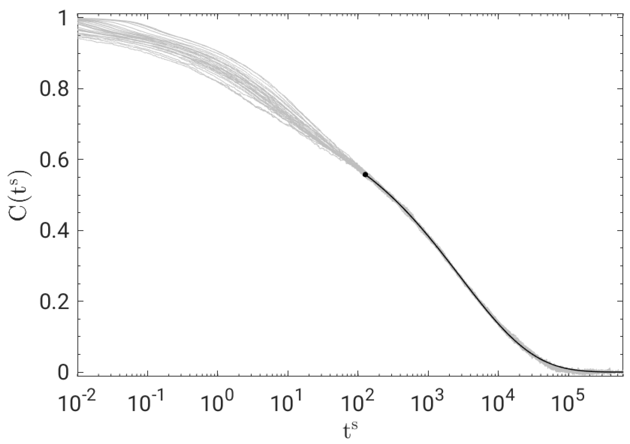
At long times, the shape of the BCF decay does not depend on the physical state. To show that, Figure 2 plots the master curve obtained by shifting the curves of Figure 1 horizontally, resulting in a remarkable time–temperature–pressure superposition (TTPS) in the time window of primary relaxation for . The best fit of the master curve with the stretched exponential , where A is an adjustable constant, yields .
TTPS motivated us to fit the whole BCF decay using different fit functions ensuring decay with constant stretching at long times. First, we adopted a weighted sum of two stretched exponentials, accounting for the primary (p) and the secondary (s) JG relaxation:
where , is Equation (2) with , . We set so as to leave Equation (8) with five adjustable parameters, i.e., . The best-fit procedure yields excellent agreement, as shown in Figure 1.
3.3. Dynamic Heterogeneity
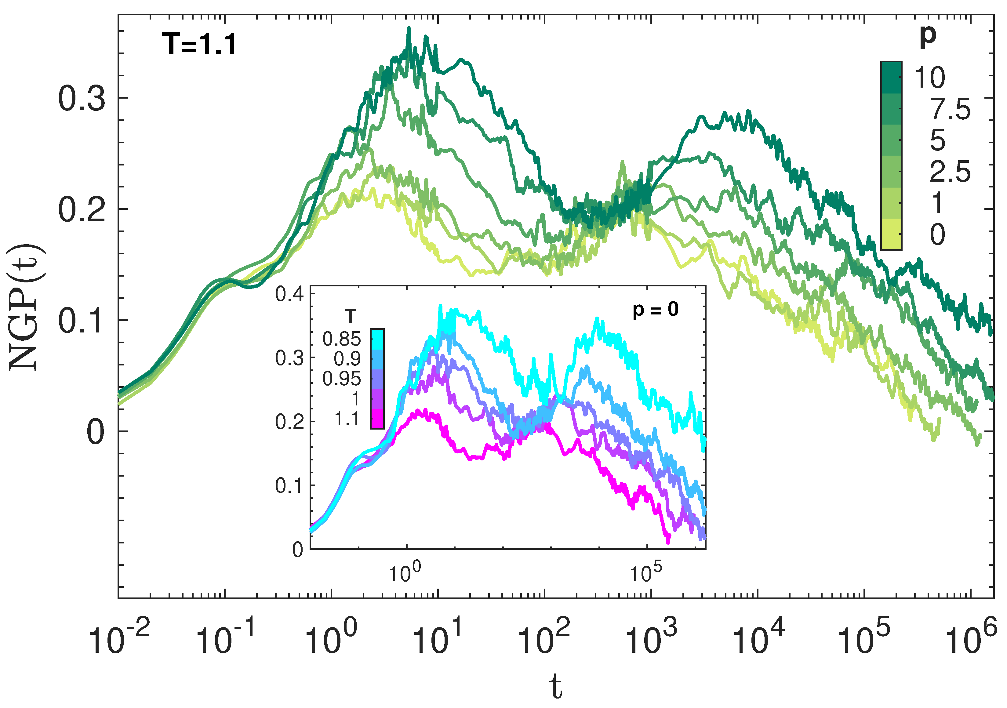
Figure 4 plots the NGP of the states in Figure 1 and shows how their DH develops with time. As in other studies, NGP is largely independent of at very short times (), suggesting a major role of static structure [35]. The small peak at about marks the average time between two consecutive collisions of the monomer with the cage formed by the closest neighbours [52]. For , NGP is strongly dependent on . Two peaks are observed, the one occurring at a shorter time attributed to the JG heterogeneity whereas the one located at longer times are due to the familiar DH of the primary, structural relaxation [36]. The height of the NGP parameter in the JG region is not surprising, given the considerable stretching of the JG relaxation seen in Figure 3.
3.4. Fractional Coupling of Primary and JG Relaxations
We now test the possible correlation between the time scales of the primary, , and the secondary JG, , relaxation processes. Figure 5 shows the result by fitting the BCF in terms of Equation (8). The correlation is excellent (Pearson correlation coefficient ) and well-expressed by a power law with exponent .
To test the robustness of the result, we fit BCF with other functions with the same number of adjustable parameters. No significant changes were observed, i.e., and exhibit excellent power-law correlation with rather similar exponent. As an example, we considered the Williams ansatz [35,53,54,55,56]:
which leads to (). Furthermore, following [16,35,55,56], we replaced in Equation (8) with the Mittag–Leffler function:
with
where is the gamma function. This leads to (). If the same replacement is performed in Equation (9), we find ().
4. Discussion
The strong power-law correlation between the primary and the JG relaxation, evidenced by Figure 5, is the key result of the present work. The power-law coupling between different time scales in systems with significant DH is documented, a well-known example being the breakdown of the Stokes–Einstein relation [26,57].
The coupling model (CM) offers a highly investigated conceptual framework predicting, according to Equation (4), the fractional coupling between the JG and the primary relaxation. Notably, if TTPS holds, the stretching parameter of the primary relaxation is independent of the state and the fractional coupling reduces to a power law between and with exponent (). Indeed, the polymer model under study exhibits TTPS, Figure 2, and a power-law correlation between and in the investigated range, Figure 5, with exponent . These findings are fully consistent with CM. However, the exponent of the power law () differs from the stretching parameter of the primary relaxation ().
To the present level of understanding, the disagreement is not easily interpreted. We offer some tentative routes to be explored in future studies. First, notably, while the well-known phenomenon of DH on the time scale of the primary (structural ) relaxation plays a central role in CM via the stretched relaxation, Equation (2), the influence of much less investigated DH on the JG time scale, which is evidenced in the present and previous studies [36], is not apparent in CM. Furthermore, we notice that CM is quite generic, i.e., the predictions are independent of the relaxation process involved in the correlation function . However, if the torsional autocorrelation function is studied by MD simulations of a polymer model which is rather similar to the present one, one finds a power law between JG and primary relaxation with an exponent ∼0.25 (see Figure 7 in ref. [51]), which is almost three times less than ours () by considering BCF. This finding suggests that, even if the power-law coupling is robust, i.e., it is revealed by different correlation functions, and captured by CM, the exponent of the power law and the stretching could depend on the particular relaxation process in a different way. Unfortunately, no information about the possible TTPS and the stretching parameter of the primary relaxation is given in ref. [51], thus hampering a closer comparison with the present study. We noted elsewhere that BCF is more sensitive to the JG relaxation than the torsional autocorrelation function in the polymer model of the present study [48].
The influence of both the choice of the correlation function, as well as the magnitude of DH in JG relaxation, on the observation of the fractional coupling between the primary and the JG relaxation is postponed to future systematic studies.
5. Conclusions
A polymer model exhibiting heterogeneous JG secondary relaxation was studied by extensive MD simulations of states with different temperature and pressure. The TTPS of the primary (segmental) relaxation is evidenced. The time scales of the primary and the JG relaxations are found to be highly correlated according to a power law in agreement with CM predictions. Nonetheless, the exponent of the power law, even if it is in the CM range (), deviates from the expected one. This motivates further investigation of the particular relaxation process involved in the correlation function addressed by CM and the heterogeneity of the JG process.
Author Contributions
Conceptualization, C.A.M., F.P. and D.L.; methodology, validation, formal analysis, investigation, C.A.M., F.P. and D.L.; software, C.A.M. and F.P.; writing—review and editing, C.A.M., F.P. and D.L.; supervision, F.P. and D.L. All authors have read and agreed to the published version of the manuscript.
Funding
A generous grant of computing time from Green Data Center of the University of Pisa, and Dell EMC® Italia is gratefully acknowledged. F.P. acknowledges funding from the European Union’s Horizon 2020 research and innovation programme under the Marie Sklodowska-Curie grant agreement No. 754496.
Institutional Review Board Statement
Not applicable.
Informed Consent Statement
Not applicable.
Data Availability Statement
The data presented in this study are available on request from the corresponding author.
Acknowledgments
Gianfranco Cordella and Antonio Tripodo are warmly thanked for helpful discussions.
Conflicts of Interest
The authors declare no conflict of interest.
Abbreviations
The following abbreviations are used in this manuscript:
| BCF | Bond correlation function |
| CM | Coupling model |
| DH | Dynamical heterogeneity |
| JG | Johari–Goldstein |
| KWW | Kohlrausch–Williams–Watts |
| LJ | Lennard–Jones |
| MD | Molecular dynamics |
| NGP | Non-Gaussian parameter |
| NPT | Constant number of monomers N, constant pressure P and constant temperature T |
| NVT | Constant number of monomers N, constant volume V and constant temperature T |
| TTPS | Time–temperature–pressure superposition |
References
- Debenedetti, P.G. Metastable Liquids; Princeton University Press: Princeton, NJ, USA, 1997. [Google Scholar]
- McCrum, N.G.; Read, B.E.; Williams, G. Anelastic and Dielectric Effects in Polymeric Solids; Dover Publications: New York, NY, USA, 1991. [Google Scholar]
- Angell, C.A.; Ngai, K.L.; McKenna, G.B.; McMillan, P.; Martin, S.W. Relaxation in glassforming liquids and amorphous solids. J. Appl. Phys. 2000, 88, 3113–3157. [Google Scholar] [CrossRef] [Green Version]
- Ngai, K.L. Relaxation and Diffusion in Complex Systems; Springer: Berlin/Heidelberg, Germany, 2011. [Google Scholar]
- Johari, G.P.; Goldstein, M. Viscous Liquids and the Glass Transition. II. Secondary Relaxations in Glasses of Rigid Molecules. J. Chem. Phys. 1970, 53, 2372. [Google Scholar] [CrossRef]
- Ngai, K.L. Relation between some secondary relaxations and the α relaxations in glass-forming materials according to the coupling model. J. Chem. Phys. 1998, 109, 6982–6994. [Google Scholar] [CrossRef]
- Ngai, K.L.; Paluch, M. Classification of secondary relaxation in glass-formers based on dynamic properties. J. Chem. Phys. 2004, 120, 857–873. [Google Scholar] [CrossRef]
- Capaccioli, S.; Paluch, M.; Prevosto, D.; Wang, L.M.; Ngai, K.L. Many-Body Nature of Relaxation Processes in Glass-Forming Systems. J. Phys. Chem. Lett. 2012, 3, 735–743. [Google Scholar] [CrossRef]
- Cicerone, M.T.; Zhong, Q.; Tyagi, M. Picosecond Dynamic Heterogeneity, Hopping, and Johari-Goldstein Relaxation in Glass-Forming Liquids. Phys. Rev. Lett. 2014, 113, 117801. [Google Scholar] [CrossRef] [Green Version]
- Yu, H.-B.; Richert, R.; Samwer, K. Structural rearrangements governing Johari-Goldstein relaxations in metallic glasses. Sci. Adv. 2017, 3, 1701577. [Google Scholar] [CrossRef] [Green Version]
- Boyd, R.H.; Breitling, S.M. The Conformational Analysis of Crankshaft Motions in Polyethylene. Macromolecules 1974, 7, 855–862. [Google Scholar] [CrossRef]
- Paul, W.; Smith, G.D.; Yoon, D.Y. Static and Dynamic Properties of a n-C100H202 Melt from Molecular Dynamics Simulations. Macromolecules 1997, 30, 7772–7780. [Google Scholar] [CrossRef]
- Meier, R.J.; Struik, L. Atomistic modelling study of relaxation processes in polymers: The β-relaxation in polyvinylchloride. Polymer 1998, 39, 31–38. [Google Scholar] [CrossRef]
- Goldstein, M. The past, present, and future of the Johari–Goldstein relaxation. J. Non-Cryst. Solids 2011, 357, 249–250. [Google Scholar] [CrossRef]
- Johari, G.P. Source of JG-Relaxation in the Entropy of Glass. J. Phys. Chem. B 2019, 123, 3010–3023. [Google Scholar] [CrossRef]
- Smith, G.D.; Bedrov, D. Relationship between the α- and β-relaxation processes in amorphous polymers: Insight from atomistic molecular dynamics simulations of 1,4-polybutadiene melts and blends. J. Polym. Sci. Part B Polym. Phys. 2007, 45, 627–643. [Google Scholar] [CrossRef]
- Karmakar, S.; Dasgupta, C.; Sastry, S. Short-Time Beta Relaxation in Glass-Forming Liquids Is Cooperative in Nature. Phys. Rev. Lett. 2016, 116, 085701. [Google Scholar] [CrossRef] [Green Version]
- Ngai, K.L.; Capaccioli, S.; Paluch, M.; Wang, L. Clarifying the nature of the Johari-Goldstein β-relaxation and emphasising its fundamental importance. Philos. Mag. 2020, 100, 2596–2613. [Google Scholar] [CrossRef]
- Johari, G.P. Glass Transition and Secondary Relaxations in Molecular Liquids and Crystals. Ann. N. Y. Acad. Sci. 1976, 279, 117–140. [Google Scholar] [CrossRef]
- Bershtein, V.; Egorov, V.; Egorova, L.; Ryzhov, V. The role of thermal analysis in revealing the common molecular nature of transitions in polymers. Thermochim. Acta 1994, 238, 41–73. [Google Scholar] [CrossRef]
- Böhmer, R.; Diezemann, G.; Geil, B.; Hinze, G.; Nowaczyk, A.; Winterlich, M. Correlation of Primary and Secondary Relaxations in a Supercooled Liquid. Phys. Rev. Lett. 2006, 97, 135701. [Google Scholar] [CrossRef]
- Goldstein, M. Communications: Comparison of activation barriers for the Johari–Goldstein and alpha relaxations and its implications. J. Chem. Phys. 2010, 132, 041104. [Google Scholar] [CrossRef]
- Cicerone, M.T.; Tyagi, M. Metabasin transitions are Johari-Goldstein relaxation events. J. Chem. Phys. 2017, 146, 054502. [Google Scholar] [CrossRef]
- Wang, B.; Zhou, Z.Y.; Guan, P.F.; Yu, H.B.; Wang, W.H.; Ngai, K.L. Invariance of the relation between α relaxation and β relaxation in metallic glasses to variations of pressure and temperature. Phys. Rev. B 2020, 102, 094205. [Google Scholar] [CrossRef]
- Sillescu, H. Heterogeneity at the glass transition: A review. J. Non-Cryst. Solids 1999, 243, 81–108. [Google Scholar] [CrossRef]
- Ediger, M.D. Spatially heterogeneous dynamics in supercooled liquids. Annu. Rev. Phys. Chem. 2000, 51, 99–128. [Google Scholar] [CrossRef] [Green Version]
- Richert, R. Heterogeneous dynamics in liquids: Fluctuations in space and time. J. Phys. Condens. Matter 2002, 14, R703–R738. [Google Scholar] [CrossRef]
- Berthier, L.; Biroli, G. Theoretical perspective on the glass transition and amorphous materials. Rev. Mod. Phys. 2011, 83, 587–645. [Google Scholar] [CrossRef] [Green Version]
- Karmakar, S.; Dasgupta, C.; Sastry, S. Length scales in glass-forming liquids and related systems: A review. Rep. Prog. Phys. 2015, 79, 016601. [Google Scholar] [CrossRef]
- Tracht, U.; Wilhelm, M.; Heuer, A.; Feng, H.; Schmidt-Rohr, K.; Spiess, H.W. Length Scale of Dynamic Heterogeneities at the Glass Transition Determined by Multidimensional Nuclear Magnetic Resonance. Phys. Rev. Lett. 1998, 81, 2727–2730. [Google Scholar] [CrossRef]
- Colmenero, J.; Alvarez, F.; Arbe, A. Self-motion and the α relaxation in a simulated glass-forming polymer: Crossover from Gaussian to non-Gaussian dynamic behavior. Phys. Rev. E 2002, 65, 041804. [Google Scholar] [CrossRef]
- Napolitano, S.; Capponi, S.; Vanroy, B. Glassy dynamics of soft matter under 1D confinement: How irreversible adsorption affects molecular packing, mobility gradients and orientational polarization in thin films. Eur. Phys. J. E 2013, 36, 61. [Google Scholar] [CrossRef]
- Napolitano, S.; Glynos, E.; Tito, N.B. Glass transition of polymers in bulk, confined geometries, and near interfaces. Rep. Prog. Phys. 2017, 80, 036602. [Google Scholar] [CrossRef]
- Weeks, E.R.; Crocker, J.C.; Levitt, A.C.; Schofield, A.; Weitz, D.A. Three-Dimensional Direct Imaging of Structural Relaxation Near the Colloidal Glass Transition. Science 2000, 287, 627–631. [Google Scholar] [CrossRef] [PubMed] [Green Version]
- Fragiadakis, D.; Roland, C.M. Role of structure in the α and β dynamics of a simple glass-forming liquid. Phys. Rev. E 2017, 95, 022607. [Google Scholar] [CrossRef] [PubMed] [Green Version]
- Puosi, F.; Tripodo, A.; Malvaldi, M.; Leporini, D. Johari–Goldstein Heterogeneous Dynamics in a Model Polymer. Macromolecules 2021, 54, 2053–2058. [Google Scholar] [CrossRef]
- Hansen, J.P.; McDonald, I.R. Theory of Simple Liquids, 3rd ed.; Academic Press: New York, NY, USA, 2006. [Google Scholar]
- Zorn, R. Deviation from Gaussian behavior in the self-correlation function of the proton motion in polybutadiene. Phys. Rev. B 1997, 55, 6249–6259. [Google Scholar] [CrossRef]
- Doi, M.; Edwards, S.F. The Theory of Polymer Dynamics; Clarendon Press: Oxford, UK, 1988. [Google Scholar]
- Kremer, K.; Grest, G.S. Dynamics of entangled linear polymer melts: A molecular-dynamics simulation. J. Chem. Phys. 1990, 92, 5057–5086. [Google Scholar] [CrossRef]
- Kröger, M. Simple models for complex nonequilibrium fluids. Phys. Rep. 2004, 390, 453–551. [Google Scholar] [CrossRef]
- Plimpton, S. Fast Parallel Algorithms for Short-Range Molecular Dynamics. J. Comput. Phys. 1995, 117, 1–19. [Google Scholar] [CrossRef] [Green Version]
- Available online: http://lammps.sandia.gov (accessed on 30 October 2022).
- Allen, M.P.; Tildesley, D.J. Computer Simulations of Liquids, 2nd ed.; Oxford University Press: Oxford, UK, 2017. [Google Scholar]
- Richter, D.; Monkenbusch, M.; Arbe, A.; Colmenero, J.; Farago, B. Dynamic structure factors due to relaxation processes in glass-forming polymers. Phys. B Condens. Matter 1997, 241–243, 1005–1012. [Google Scholar] [CrossRef]
- Tölle, A. Neutron scattering studies of the model glass former ortho-terphenyl. Rep. Prog. Phys. 2001, 64, 1473–1532. [Google Scholar] [CrossRef] [Green Version]
- Fragiadakis, D.; Roland, C.M. Dynamic correlations and heterogeneity in the primary and secondary relaxations of a model molecular liquid. Phys. Rev. E 2014, 89, 052304. [Google Scholar] [CrossRef]
- Tripodo, A.; Puosi, F.; Malvaldi, M.; Capaccioli, S.; Leporini, D. Coincident Correlation between Vibrational Dynamics and Primary Relaxation of Polymers with Strong or Weak Johari-Goldstein Relaxation. Polymers 2020, 12, 761. [Google Scholar] [CrossRef] [PubMed] [Green Version]
- Barbieri, A.; Campani, E.; Capaccioli, S.; Leporini, D. Molecular dynamics study of the thermal and the density effects on the local and the large-scale motion of polymer melts: Scaling properties and dielectric relaxation. J. Chem. Phys. 2004, 120, 437–453. [Google Scholar] [CrossRef] [PubMed] [Green Version]
- Bedrov, D.; Smith, G.D. Molecular dynamics simulation study of the α and β-relaxation processes in a realistic model polymer. Phys. Rev. E 2005, 71, 050801. [Google Scholar] [CrossRef] [PubMed]
- Bedrov, D.; Smith, G.D. Secondary Johari–Goldstein relaxation in linear polymer melts represented by a simple bead-necklace model. J. Non-Cryst. Solids 2011, 357, 258–263. [Google Scholar] [CrossRef]
- De Michele, C.; Leporini, D. Viscous flow and jump dynamics in molecular supercooled liquids. I. Translations. Phys. Rev. E 2001, 63, 036701. [Google Scholar] [CrossRef]
- Williams, G. Molecular aspects of multiple dielectric relaxation processes in solid polymers. In Proceedings of the Electric Phenomena in Polymer Science. In Advances in Polymer Science; Springer: Berlin/Heidelberg, Germany, 1979; pp. 59–92. [Google Scholar]
- Williams, G. Dielectric relaxation spectroscopy of polymers revealing dynamics in isotropic and anisotropic stationary systems and changes in molecular mobility in non-stationary systems. Polymer 1994, 35, 1915–1922. [Google Scholar] [CrossRef]
- Fragiadakis, D.; Roland, C.M. Characteristics of the Johari-Goldstein process in rigid asymmetric molecules. Phys. Rev. E 2013, 88, 042307. [Google Scholar] [CrossRef] [Green Version]
- Fragiadakis, D.; Roland, C.M. Rotational dynamics of simple asymmetric molecules. Phys. Rev. E 2015, 91, 022310. [Google Scholar] [CrossRef] [Green Version]
- Chang, I.; Fujara, F.; Geil, B.; Heuberger, G.; Mangel, T.; Sillescu, H. Translational and rotational molecular motion in supercooled liquids studied by NMR and forced Rayleigh scattering. J. Non-Cryst. Solids 1994, 172–175, 248–255. [Google Scholar] [CrossRef]
Figure 1.
Isothermal and isobaric (inset) plots of selected BCFs, Equation (7). The superimposed thin solid black lines are the best fit with Equation (8).

Figure 2.
Time−temperature−pressure superposition (TTPS) of BCF for all the states in Figure 1. The curves are shifted along the horizontal axis to optimise their superposition at long times. The superimposed solid black line is the best fit with a stretched exponential proportional to , Equation (2), with .

Figure 3.
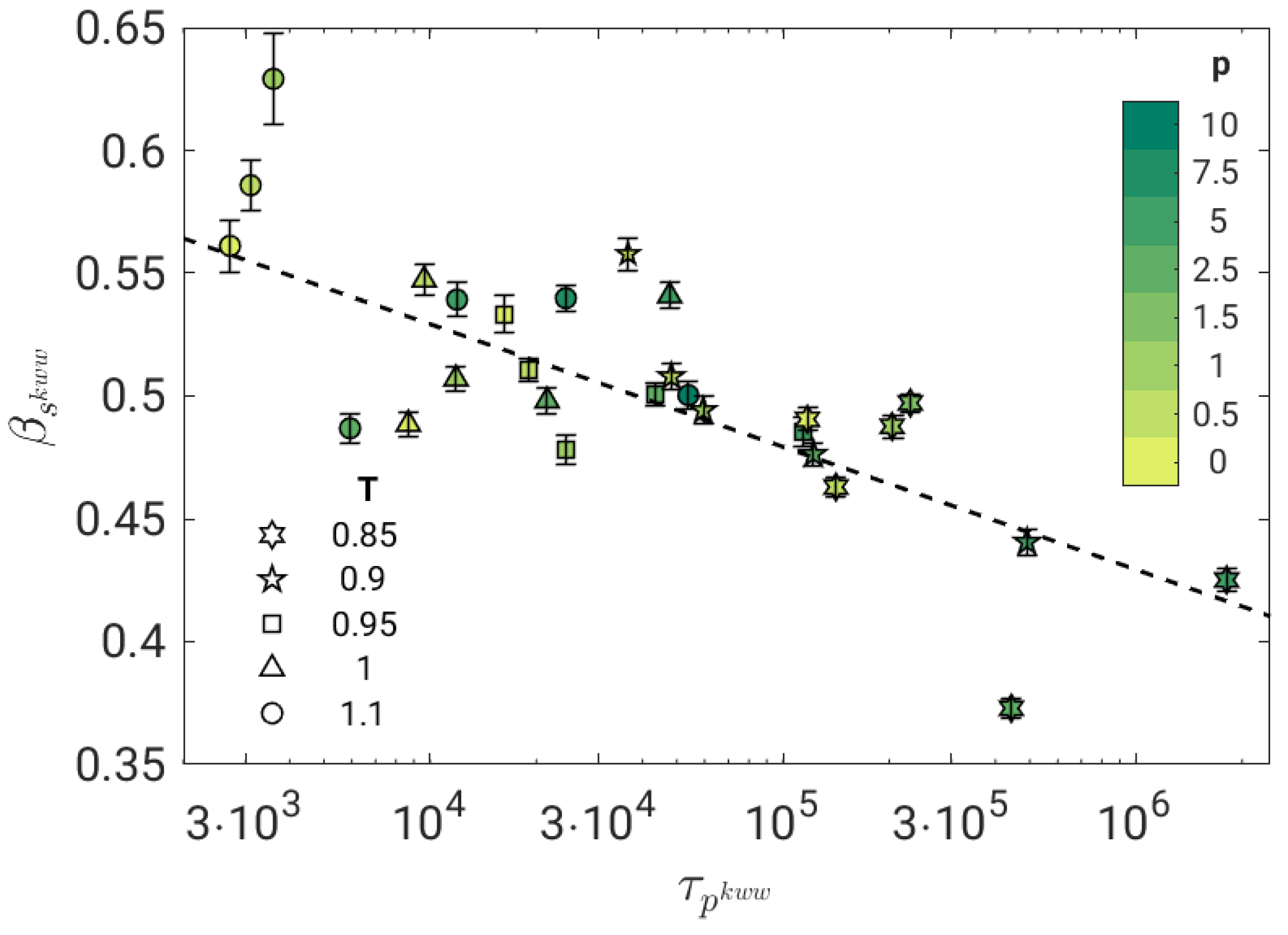
Stretching parameter of the secondary JG relaxation of all the investigated states according to the best fit with Equation (8). The dashed line is a guide for the eyes. Stretching increases mildly with the primary relaxation time.
Figure 3.
Stretching parameter of the secondary JG relaxation of all the investigated states according to the best fit with Equation (8). The dashed line is a guide for the eyes. Stretching increases mildly with the primary relaxation time.

Figure 4.
NGP, Equation (5), of all the states in Figure 1. DH is apparent in both the secondary JG relaxation time scale, t∼1–10, and the the primary, segmental relaxation, t∼–.

Figure 5.
Correlation plot between the JG relaxation time and the primary relaxation time of all the investigated states, as drawn by fitting BCF with a weighed superposition of two stretched exponentials, Equation (8). The correlation is excellent (Pearson correlation coefficient ) and best fit with a power law with slope (dashed line). The grey area is the confidence region within one standard deviation of the best-fit parameters.


Table 1.
Investigated temperature and pressure values.
| T∖p | 0 | 0.5 | 1 | 1.5 | 2.5 | 5 | 7.5 | 10 |
|---|---|---|---|---|---|---|---|---|
| 1.1 | ||||||||
| 1 | ||||||||
| 0.95 | ||||||||
| 0.9 | ||||||||
| 0.85 |
Publisher’s Note: MDPI stays neutral with regard to jurisdictional claims in published maps and institutional affiliations. |
© 2022 by the authors. Licensee MDPI, Basel, Switzerland. This article is an open access article distributed under the terms and conditions of the Creative Commons Attribution (CC BY) license (https://creativecommons.org/licenses/by/4.0/).
Share and Cite
MDPI and ACS Style
Massa, C.A.; Puosi, F.; Leporini, D. Fractional Coupling of Primary and Johari–Goldstein Relaxations in a Model Polymer. Polymers 2022, 14, 5560. https://0-doi-org.brum.beds.ac.uk/10.3390/polym14245560
AMA Style
Massa CA, Puosi F, Leporini D. Fractional Coupling of Primary and Johari–Goldstein Relaxations in a Model Polymer. Polymers. 2022; 14(24):5560. https://0-doi-org.brum.beds.ac.uk/10.3390/polym14245560
Chicago/Turabian StyleMassa, Carlo Andrea, Francesco Puosi, and Dino Leporini. 2022. "Fractional Coupling of Primary and Johari–Goldstein Relaxations in a Model Polymer" Polymers 14, no. 24: 5560. https://0-doi-org.brum.beds.ac.uk/10.3390/polym14245560
Note that from the first issue of 2016, this journal uses article numbers instead of page numbers. See further details here.