Metric Map Generation for Autonomous Field Operations

Abstract

Advanced systems for manned and/or agricultural vehicles—such as systems for auto-steering, navigation-adding, and autonomous route planning—require new capabilities in terms of the internal representation for the autonomous system of the working space; that is, the generation of a metric map that provides by numerical parameters any operation-related entity of the working space. In this paper, a real-time approach was developed for the generation of the field metric map, based on a row generation method (polygons-based geometry). The approach can deal with fields with or without in-field obstacles, where the generated field-work tracks can be either straight or curved. The functionality of the approach was demonstrated on 12 fields with different number of obstacles ranging from one to six. The test results showed that the computational times were in the range of 0.26–24.51 s. The presented tool brings a number of advancements on the process of generating a metric map for arable farming field operations, including the real-time generation feature, the potential to deal with multiple-obstacle areas, and the reduction in the overlapped area.

1. Introduction

Agriculture faces a range of social and environmental challenges, such as the growing demand for high-quality food products, climate change, and market globalization. Farmers are forced to reduce production cost while maximizing the quality of products in order to compete in the globalized market [1]. Machinery investment, maintenance, and operational usage are key parts of the production costs. In order to enhance machinery productivity and operational efficiency, and consequently to reduce production costs, increasing efforts are being contributed to the development of advanced operations management systems using advanced information technologies, automation, sensing systems, and actuating systems [2,3,4,5].

As part of these aforementioned efforts, a significant amount of research has been dedicated to the development of advanced algorithms or methods for automating operations optimization in arable farming. This has included various approaches for the improvement of the field efficiency of semi-automated operations (navigation-adding systems) or fully autonomous (field robots) operations, and these approaches include route planning and field area coverage [6,7,8,9,10,11,12,13,14,15,16,17,18]. However, the transition of field operations from manual operated operations to fully automated operations requires new functionalities of the developed operations optimisation systems.

To this direction, a significant amount of research has been dedicated to the development of advanced algorithms or methods for automating operations optimization in arable farming. This has included various approaches for the improvement of the efficiency of field automated (navigation-adding systems) or autonomous (field robots) operations, such as route planning and field area coverage approaches [6,7,8,9,10,11,12,13,14,15,16,17,18]. However, the modification of the processes from conventional to fully automated operation requires new functionalities of the developing systems.

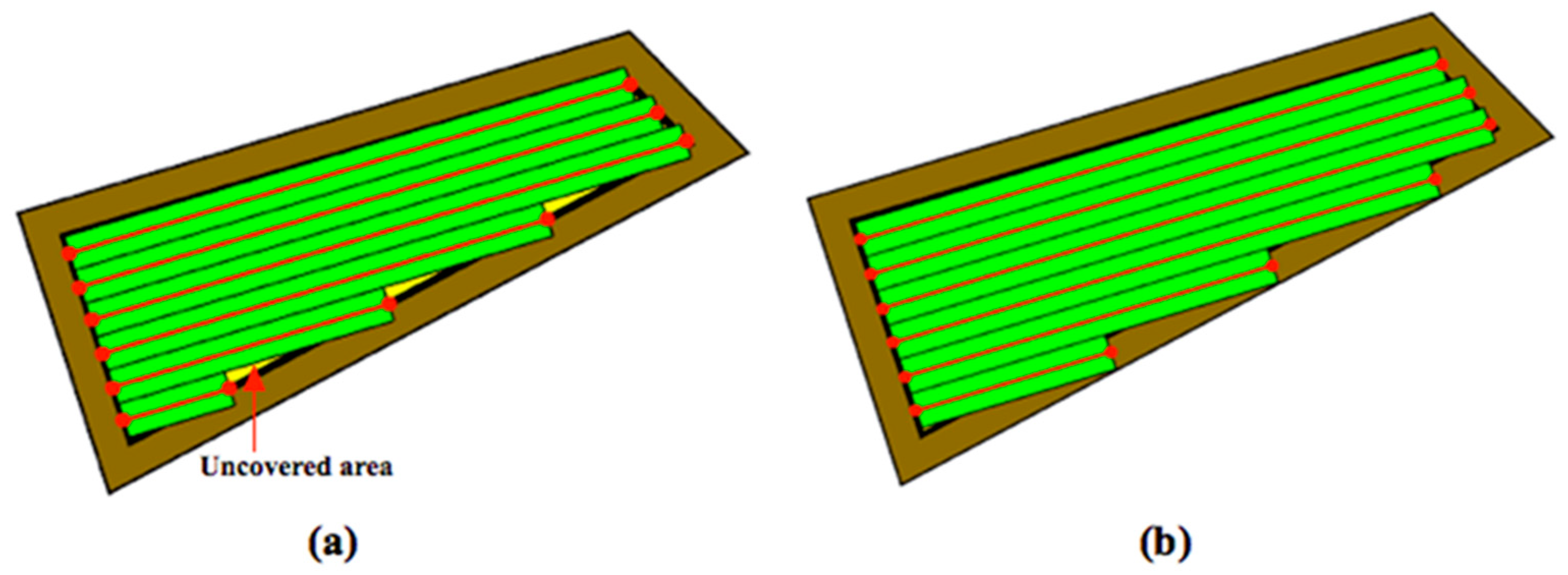
The execution of autonomous operations requires a “world representation”, that is a geometrical representation of working space for the autonomous system. This usually includes the use or the generation of a metric map that provides by numerical parameters the representation of any operation-related entity of the working space. In the general mobile robotics case, this metric map could be either a Cartesian (geometrical) map or a grid-based map. However, in agricultural operations, due to the constrained vehicle traversal of the field (i.e., moving on pre-defined field-work tracks), all of the approaches regard the generation of a geometrical map. A number of methods have been introduced for the generation of geometrical representation of either simple convex or complex concave fields. For example, Palmer et al. (2003) generated predefined field-work tracks aiming to reduce the amount of overlapped and missed area [19]. Taïx et al. (2006) proposed algorithms to generate straight field-work tracks for field coverage both in the cases of convex or non-convex fields without obstacles [20]. Algorithms for the generation of field representations for complex fields have been developed by Oksanen and Visala (2007), in which, firstly, complex fields were divided into simple trapezoid fields, then straight field-work tracks were generated, based on a calculated driving direction derived from the function of working width and turning time [21]. Hameed et al. (2010) presented a mathematically descripted method for the generation of field geometrical representations in real time for fields with or without obstacles using straight or curved field tracks [22]. Spekken et al. (2016) presented a method to generate patterns of fieldwork tracks in the form of curved polylines on sloping land to assess their susceptibility to water erosion [12]. Hameed et al. (2016) presented an approach for a 3D coverage map generation, where the 2D coverage map is projected through field terrain [23]. The selected test fields showed savings of skipped and overlapped areas in the range of 2%–14%. However, all methods have some limitations in terms of completeness. Tracks generated in the various methods only intersect with the inner boundary of the field or the outer boundary of obstacles, as shown Figure 1a. It can be seen that following these generated field-work tracks by agricultural vehicles will lead to uncovered areas (yellow colored area). Therefore, in order to cover the entire field, these tracks have to be extended by some distance as shown in Figure 1b. The process of tracks extension becomes complicated when a field comprises multiple obstacles.

To this end, in this paper a new algorithmic method for the generation of a metric map representing an agricultural field using headland field work pattern is presented. In this method, a row generation-based approach (polygons-based geometry) is implemented to eliminate the uncovered areas as illustrated in Figure 1a. The generated fieldwork tracks can be either straight or curved field-work tracks for any complexity level of fields in terms of shape and number of in-field obstacles. It should be noted that the presented approach aims to provide partial improvements in the problem of metric map generation for field autonomous operation and not yet a complete solution. This is due to various limitations of the approach which are presented in the Discussion Section.

2. Methods

In this section, firstly, the applied geometric primitives are explained and defined in Section 2.1. Next, various geometric operators used for manipulation of geometric primitives are introduced in Section 2.2. Lastly, the procedures of generating field geometrical representation are presented in details in Section 2.3.

2.1. Geometric Primitives

Polyline. A polyline, $l$, is an ordered path composed of a collection of contiguous line segments $l=\langle l_{x_1{x}_2},l_{x_2{x}_3},\dots ,l_{x_{n-1}{x}_n}\rangle$. A line segment is a special case of a polyline with $n=2$.

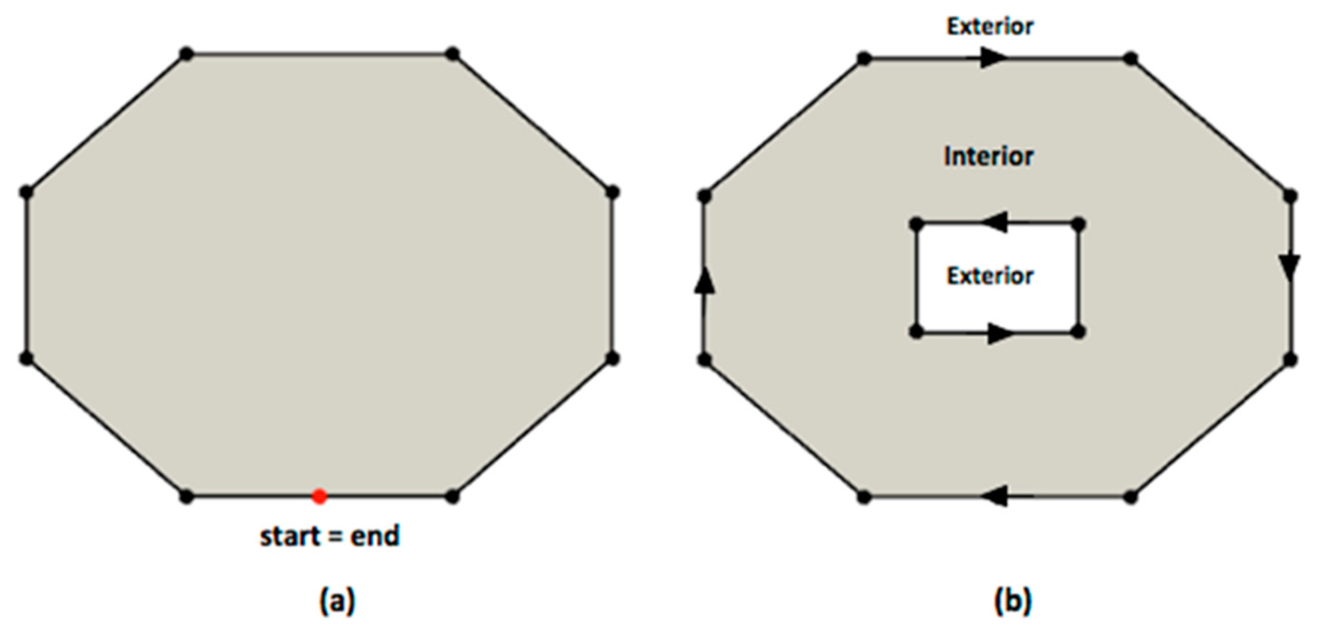
Polygon. A polygon, $p$, is defined by a collection of rings, $p=\langle r_1,r_2\dots r_n\rangle , n\ge 1$, where a ring, $r$, is defined by a collection of contiguous ordered line segments, $r=\langle l_{x_1{x}_2},l_{x_2{x}_3}\dots l_{x_n{x}_1}\rangle$, such that the start and end points are the same point, as depicted in Figure 2a.

A polygon has one outer ring $r_1$ and zero or multiple inner rings $\left\{r_2,\dots ,r_n\right\}$. The outer ring $r_1$ is oriented clockwise while an inner ring $r_i, i\in \left\{2,\dots ,n\right\}$ is oriented counter-clockwise (see Figure 2b). Following this orientation, the area to the right of the outer ring and the inner rings defines the interior (shaded part in Figure 2) of the polygon. Similarly, the area to the left of the rings is the exterior of the polygon. In our study, the field boundary is equivalent to the outer ring, the obstacle boundary is equivalent to an inner ring, and the field body $F_b$ (the operational area) is equivalent to the interior polygon area.

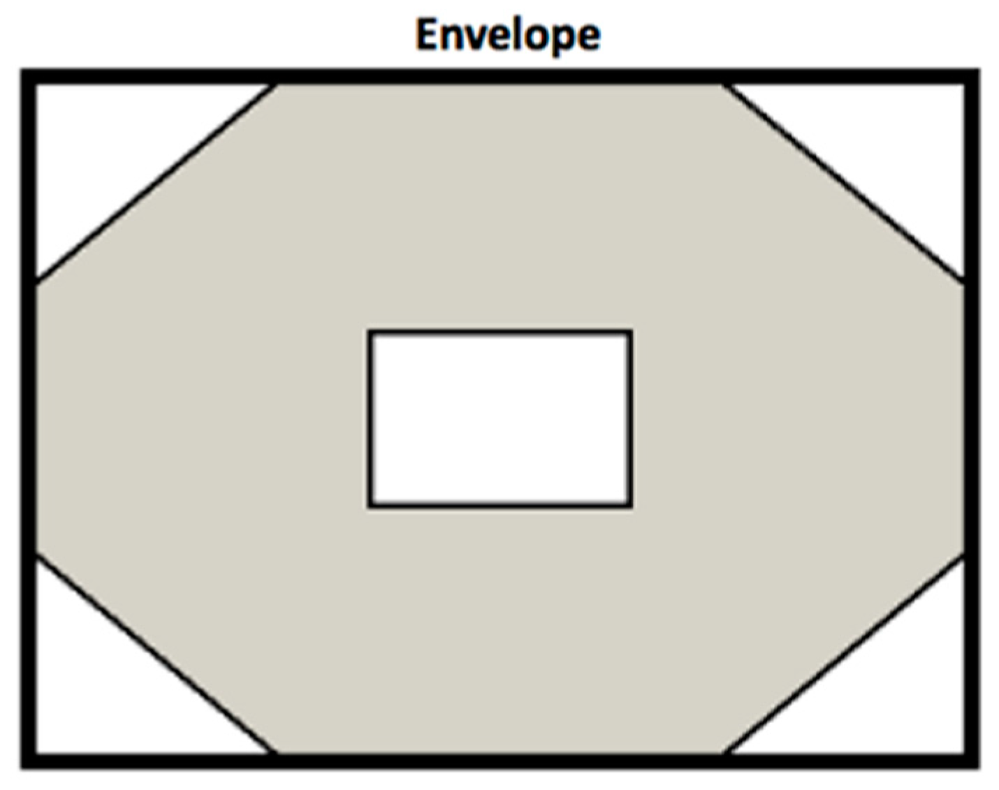
Envelope. An envelope, $e$, is a bounding rectangle that encloses a geometry $g\in \left\{l, r, p\right\}$. A given geometry $g$ can have multiple bounding rectangles with different orientation angle. The minimum bounding rectangle $e_{min}$ (as shown in Figure 3) has the smallest area among all the bounding rectangles.

2.2. Geometric Operators

Intersection ($\mathbf{\cap }\mathbf{\left(}A\mathbf{,}B\mathbf{\right)}$). The intersection operator $\cap$ is used to find the overlapped area $g$ between two geometries $\mathsf{{\rm A}}$ and $\mathsf{{\rm B}}$. The geometries can be line segments, polylines, rings or polygons. If $g$ is the intersection between $\mathsf{{\rm A}}$ and $\mathsf{{\rm B}}$ it satisfies that $g\subseteq \mathrm{A}\wedge g\subseteq \mathrm{B}$. Intersection examples are illustrated in

Table 1. Illustration of intersection $\cap \left(A,B\right)$ and subtraction $\mathsf{\Delta }\left(A,B\right)$. Results of the operations are marked green.

Input Geometries	Intersection $\cap \left(A,B\right)$	Subtraction $\mathsf{\Delta } \left(A, B\right)$

where the green marked geometry corresponds to the intersection between two examples of geometries $\mathsf{{\rm A}}$ and $\mathrm{B}$.

Subtraction ($\mathsf{\Delta } \mathbf{\left(}A\mathbf{,} B\mathbf{\right)}$). The subtraction operator $\mathsf{\Delta }$ determines a geometry $g$, which is the difference between the two input geometries $\mathrm{A}$ and $\mathrm{B}$. The subtracted geometry $g$ satisfies the condition that $g\subseteq \mathrm{A}\wedge g⊈B$ and. Examples are given in Table 1. Note, that subtraction does not obey the commutative law ($\mathsf{\Delta }\left(\mathrm{A},\mathrm{B}\right)\ne \mathsf{\Delta }\left(\mathrm{B},\mathrm{A}\right)$).

Offset (${\mathbf{\parallel }}_{\mathbf{\pm }\mathit{d}}^{\mathit{g}}$). The offset operator ${\parallel }_{\pm d}^g$ creates a geometry that is parallel to the input geometry $g\in \left\{l, r, p\right\}$ at a specified distance $d$. The distance can be either positive $(+)$ or negative $(-)$. Examples of offset for a polygon, polyline and line segment are presented in

Table 2. Illustration of the offset operator for polygon, polyline and line segment with offset width $\mathit{d}$ . The direction of both lines is from bottom left to top right. The green lines and rings are the generated geometries by the offset operator ${\parallel }_{\pm \mathit{d}}^{\mathit{g}}$.

Polygon Offset	Polyline Offset	Line Offset

.

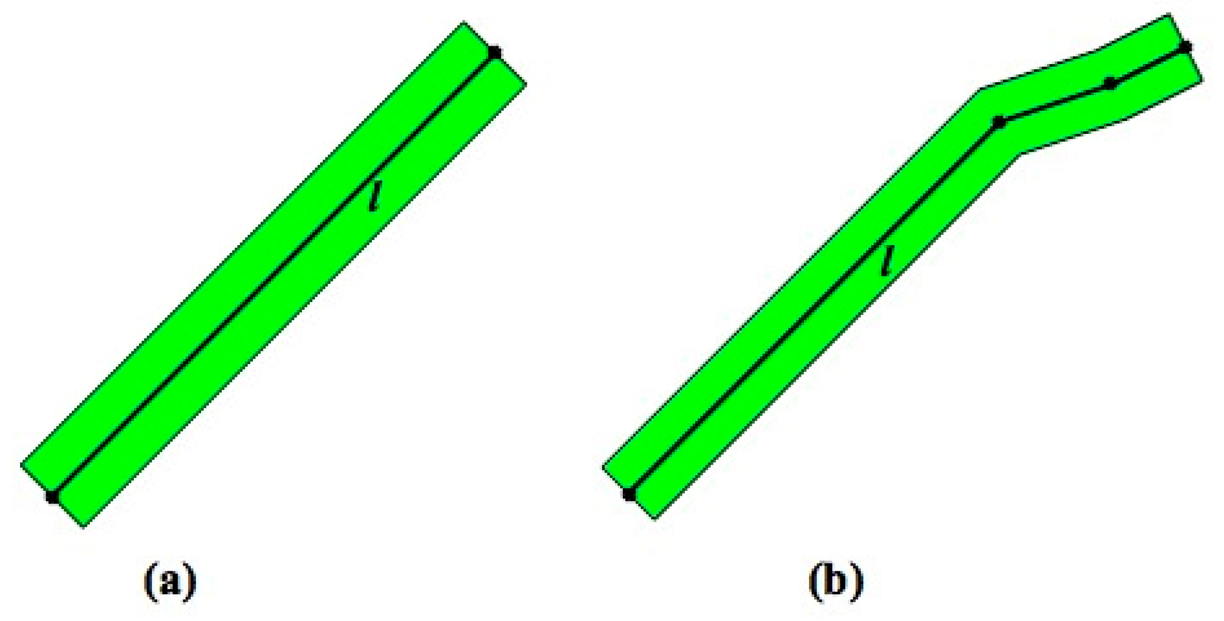
Buffer (${\mathsf{\Pi }}_{\mathit{d}}^{\mathit{l}}$). The buffer operator $\mathsf{\Pi }$ creates a polygon around the input line $l$, which may be a line segment or a polyline. First, two parallel lines to both sides of $l$ at a specified distance $d$ are generated with the offset operator ${\parallel }_{+d}^l$ and ${\parallel }_{-d}^l$, and then, these two lines are joined in the ends to compose the buffer polygon $p_{buf}$ around $l$. In the example in Figure 4, the black line is the input line$l$ and the green polygon is a buffer polygon.

Projection ($\mathbf{\perp }\mathbf{\left(}\mathit{m}\mathbf{,}\mathit{l}\mathbf{\right)}$). The projection operator, $\perp$, projects a point $m$ to a line or polyline $l$ and determines the projected point $m^{\prime }$ on $l$ such that the line $l_{m{m}^{\prime }}$ has the shortest distance to $l$. Figure 5a. illustrates how the points $m_1,m_2,m_3$ and $m_4$ are projected on the polyline $l=\langle l_{x_1{x}_2},l_{x_2{x}_3}\rangle$. Note, that $m_2$ projects to two points on $l$, $m_2^{\prime }$ and $m_2^{″}$, since $m_2$ is equidistant to the line segments $l_{x_1{x}_2}$ and $l_{x_2{x}_3}$ in Figure 5a. The projection point $m^{\prime }$ can be either interior or exterior of $l$, as illustrated in Figure 5a, where the projection points $m_1^{\prime },m_2^{\prime },m_2^{″}$ and $m_3^{\prime }$ are interior to $l$, while $m_4^{\prime }$ is exterior.

Point union ($\mathsf{⨃}\mathbf{\left(}\mathbf{\left\{}\mathit{m}\mathbf{\right\}}\mathbf{\right)}$). The point union operator $\mathsf{⨃}$ takes an ordered set of points $\left\{m\right\}$ and generates a polyline consisting of line segments with end points in $\left\{m\right\}$. In the context of this paper, the point union operator is always used along with the projection operator $\perp$ to create a line segment or a polyline that links all the projection points and points of the original line that lie in between these projection points. This is illustrated in Figure 5b, where the point union operator is used to create a new polyline $l^{\prime }=\mathsf{⨃}\left(\left\{m\right\}\right)$, where $m=\{m_1^{\prime },m_2^{\prime },x_2,m_2^{″},m_3^{\prime },x_3,m_4^{\prime }\}$.

Boolean intersect ($\mathbf{\&} \mathbf{\left(}A\mathbf{,} B\mathbf{\right)}$). The boolean intersect operator & is used to check if two geometries $A$, $B$ intersect or not, i.e., if they share at least one point.

2.3. Metric Map Generaiton

In this section, the methods for generation of the geometrical representation of a field by using the aforementioned geometric primitives and operators are introduced.

2.3.1. Inputs

The input set required for the generation of the field metric map includes:

• The boundary of the field area and the boundaries of the in-field obstacles, which are represented by a polygon, ${\mathit{p}}_{\mathit{field}}$.
• The number of headland passes ($\mathit{\eta }$) for the main field and each obstacle.
• The line (${\mathit{l}}_{\mathit{A}\mathit{B}}$), which is used as $\mathit{A}\mathit{B}$ reference line for generation of the parallel field-work tracks. ${\mathit{l}}_{\mathit{A}\mathit{B}}$ can be either a straight-line segment or a polyline.
• The operating width ($\mathit{w}$). This is the effective operating width of the implement.

2.3.2. Metric Map Entities

The representation involves the generation of the following geometric entities:

Headland passes: a headland pass is a peripheral path internally around the field boundary or externally of an obstacle. The headland area consists of the several headland passes and provides the required space for the machine turnings. The remaining field area excluding the (field and obstacle/s) headland areas and obstacle/s area/s, is called the field body area.

Field-work tracks: In order to cover the entire field body area, a set of parallel tracks has to be generated as the guidance lines for the agricultural machine. These field-work tracks can be represented either as straight-line segments or as curved polylines.

Rows: each row area is the area processed by an implement while driving along a track. The width of each row equals the effective implement width of the machine, $w$.

The overlapped area is a double covered (processed) area, which occurs at headland turnings or at the first and last row when they are doubled by the headland area.

In the following, the specific methods of the generation of these entities are described.

2.3.3. Generation of Headland Passes and Headland Areas

A headland area must be generated for the field as well as for each of its obstacles. Each headland area consists of $\eta +2$ rings, where $\eta$ is the number of headland passes, namely the field (or obstacle) boundary, the $\eta$ headland passes, and the headland boundary to the main field area (shown in Figure 6 with black, blue, and red rings, respectively). Let $r\in \{r_f,$ $r_1, \dots , r_{\theta }\}$ denote the boundary of the field and the boundaries of the $\theta$ obstacles. Let $H_r=\left\{h_1,\dots ,h_{\eta }\right\}$ denote the headland passes (blue rings in Figure 6). The first headland pass is obtained by offsetting $r$ at distance $w/2$: $h_1= {\parallel }_{+w/2}^r$. The subsequent headland passes are generated recursively by offsetting at distance $w$ from the previous headland pass: $h_i= {\parallel }_{+w}^{h_{i-1}}, i=2,\dots ,\eta$. Finally, the headland boundary ring (red rings in Figure 6) is created at a distance $w/2$ from the last headland pass $h_{\eta }$: $b= {\parallel }_{+w/2}^{h_{\eta }}$. In this way, the headland area of a field or obstacle contains the rings: $\left\{r, h_1,h_2,\dots ,h_{\eta }, b\right\}$. For the field we denote the outer and inner boundaries $r_f$ and $b_f$, respectively. The field body area $F_b$ can be obtained by using the subtraction operation $F_b$ = $\mathsf{\Delta }\left(b_f,{\sum }_{i=1}^{\theta }{b}_i\right)$, which is the enclosed area by $b_f$ excluding the total area enclosed by the obstacle inner boundary $b_i,i\in \left\{1,\dots ,\theta \right\}$.

2.3.4. Tracks and Rows Generation

In the following, the method for generating straight and curved tracks is described.

Straight field-work tracks

As a first step, in order to restrict all generated tracks inside the operational area, a bounding envelope $e$ (the green rectangle in the Figure 7a) of the field’s headland boundary ring, $b_f$, is generated with one edge $l$ of the envelope parallel to the driving direction $l_{AB}$. The edge $l$ is selected as a reference line for generating tracks. The number of field-work tracks for a complete coverage of area $e$. is given by $\tau =\lceil \left|l^{\prime }\right|/w\rceil$ where ⌈⌉ is the ceil function and $\left|l^{\prime }\right|$ is the length of the edge $l^{\prime }$ of $e$ that is perpendicular to $l$. A set $T=\left\{t_1,t_2,\dots ,t_{\tau }\right\}$ of initial line segments, each with two intersections with the bounding envelope $e$, is generated sequentially by offsetting the reference line $l$ and by implanting using the offset operator: $t_i= {\parallel }_{d= w/2+\left(i-1\right)·w}^l, i=1, 2\dots \tau$ (the black lines with dotted end points in Figure 7b).

The specific steps for the generation of the field-work tracks and the corresponding rows, includes:

• Firstly, each initial track ${\mathit{t}}_{\mathit{i}}$ is used to create a buffer polygon ${\mathit{p}}_{\mathit{buf}}$ using the buffer operator ${\mathsf{\Pi }}_{\mathit{w}/\mathbf{2}}^{ {\mathit{t}}_{\mathit{i}}}$ (Figure 8a). Then, the intersection operator is used to find the intersection area between the buffer polygon ${\mathit{p}}_{\mathit{buf}}$ and the inner field boundary ${\mathit{b}}_{\mathit{f}}$ disregarding obstacles: ${\mathit{p}}_{\mathit{int}}= \cap \left({\mathit{p}}_{\mathit{buf}},{\mathit{b}}_{\mathit{f}}\right)$ (Figure 8b).
• Next, the boolean intersect operator $\&$ is applied to check whether the ${\mathit{p}}_{\mathit{int}}$ intersects with the obstacles. Following this, there are three potential cases, as illustrated in Figure 8c: Case 1: if ${\mathit{p}}_{\mathit{int}}$ is not intersected with any obstacle, then ${\mathit{p}}_{\mathit{int}}$ remains unchanged; Case 2: if ${\mathit{p}}_{\mathit{int}}$ only partially intersects with obstacles, then the subtraction operator $\mathsf{\Delta }$ is employed to obtain the subtracted area; and Case 3: if ${\mathit{p}}_{\mathit{int}}$ crosses through an obstacle, then the subtraction operator $\mathsf{\Delta }$ divides the polygon ${\mathit{p}}_{\mathit{int}}$ into sub-polygons. Other cases such as a ${\mathit{p}}_{\mathit{int}}$ partially intersects one obstacle and crosses through another obstacle are considered as the case of the combination of basic cases 2 and 3.
• After the subtraction operation has been performed, each ${\mathit{p}}_{\mathit{fin}}$ area is enclosed by a ring with multiple points denoted as a set $\left\{\mathit{m}\right\}$ (red points in Figure 8c). To obtain the final track, ${\mathit{t}}_{\mathit{fin}}$, first, points in the set $\left\{\mathit{m}\right\}$ are projected to the initial track $\mathit{t}$ by the projection operator $\perp$ to acquire the projection points set $\left\{{\mathit{m}}^{\prime }\right\}$. Afterwards, the final track ${\mathit{t}}_{\mathit{fin}}$ (black dotted lines in Figure 9a) is created using the union operator $\mathsf{⨃}\left(\left\{{\mathit{m}}^{\prime }\right\}\right)$. In addition, the row ${\mathit{R}}_{\mathit{fin}}$ of the final track ${\mathit{t}}_{\mathit{fin}}$ (green area in Figure 9b) is generated by employing the buffer operator ${\mathsf{\Pi }}_{\mathit{w}/\mathbf{2}}^{{\mathit{t}}_{\mathit{fin}}}$.

A field representation derived from applying these three steps on each row is illustrated in Figure 9c.

The pseudo-code of the process is shown in Algorithm 1.

Algorithm 1. Pseudo-code for the generation of straight tracks and corresponding rows.

For each initial track t $ϵ\left\{t_1,t_2\dots t_{\tau }\right\}$ do

$p_{buf}$ $\leftarrow {\Pi }_{w/2}^t$  # Create a buffer around a initial track t

$p_{int}$ $\leftarrow \cap (p_{buf},b_f)$ # Obtain the intersection $p_{int}$ between $p_{buf}$ and field inner boundary area $b_f$

If  $\&(p_{int}, b_{i=\left\{1,2,\dots ,\theta \right\}}$) == false

$p_{fin}\leftarrow p_{int}$;

Else

$p_{fin}\leftarrow \Delta (p_{int},b_{i=\left\{1,2,\dots ,\theta \right\}})$; # Find the subtracted area between $p_{int}$ and inner boundary $b_{i=\left\{1,2,\dots ,\theta \right\}}$ of obstacle $r_i$.

End

For each $p_{fin}$ do

Get a set of projection points to $t$, {m′} ← $\perp \left(m,t\right)$, $m$ is the set of points that constitute $p_{fin}$;

Final track $t_{fin}$ ← $\mathsf{⨃}\left(\left\{m^{\prime }\right\}\right)$;

Row of final track $R_{fin}\leftarrow {\Pi }_{w/2}^{t_{fin}}$;

End

End

Curved field-work tracks

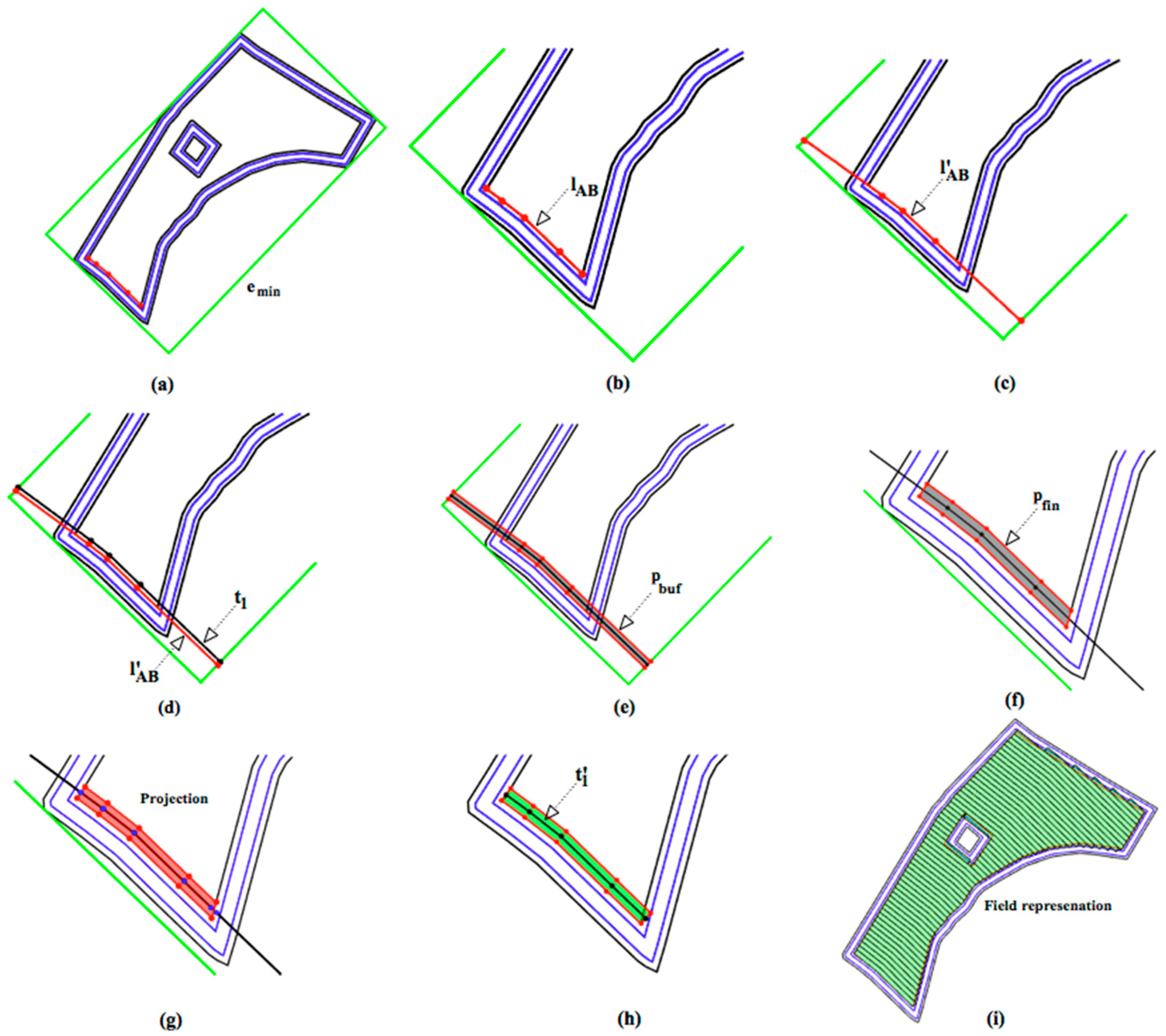
The procedure to generate a geometrical map with curved tracks is similar to the procedure for straight tracks explained above. The differences stem from the fact that the reference line $l_{AB}$ in latter case is a polyline. In the following, the procedure for generation of curved tracks is presented with reference to Figure 10.

To ensure that the operational area is fully covered with parallel, curved tracks, the minimum-bounding envelope $e_{min}$ of the outer field border, $r_f$, is used (Figure 10a). The reference line $l_{AB}$ is laid out along the inner field border, $b_f$, such that the orientation of the line follows the clockwise ordering around the field inner boundary (Figure 10b). Then, $l_{AB}$ is extended to intersect with $e_{min}$, resulting in the extended reference line, $l_{AB}^{\prime }$ (Figure 10c). Next, the first of a sequence of initial tracks $T=\left\{t_1,t_2,\dots ,t_{\tau }\right\}$ covering $e_{min}$ is generated. The first track $t_1$ is made up as an offset of $l_{AB}^{\prime }$ of a width of $w/2$: $t_1= {\parallel }_{+w/2}^{l_{AB}^{\prime }}$ (Figure 10d). Note, that since $l_{AB}^{\prime }$, like as $l_{AB}$, follows the clockwise direction it is only required to use offset to the right ($+$ for distance parameter) to make offset inwardly to operational area. The next steps are analogous to the generation of straight tracks: Generation of buffer polygon $p_{buf}$ for each track (Figure 10e); subtraction of area outside the inner field boarder and obstacle borders to obtain first $p_{int}$ and then $p_{fin}$ (Figure 10f); projection of points on $p_{fin}$ to $t_1$ (Figure 10g) to determine the final first track, $t_1^{\prime }$ and the corresponding row $R_1^{\prime }$ (Figure 10h). Having completed the first track, the subsequent initial tracks can be generated recursively from the previous final track: $t_i= {\parallel }_{+w}^{t_{i-1}^{\prime }}, i=2,\dots ,\tau .$ Then the initial track $t_i$ can be finalized into $t_i^{\prime }$ until the final tracks cover the entire operational area of the field (Figure 10i). The pseudo-code for generation of curve tracks with corresponding rows is give in Algorithm 2.

Algorithm 2. Pseudo-code for generation of curved tracks with corresponding rows.

While until no track intersects with $e_{min}$

If $i==1$

$l_{A{B}^{\prime }}\leftarrow$ Extend $l_{AB}$ to intersect with $e_{min}$;

$t_1$ = ${\parallel }_{w/2}^{{\mathit{l}}_{\mathit{A}{\mathit{B}}^{\mathbf{\prime }}}};$

$p_{buf}\leftarrow {\Pi }_{w/2}^{t_1}$  # Create a buffer around $t_1$;

Else

$t_i$ = Extend $t_{i-1}^{\prime }$ to intersect with $e_{min}$;

$p_{buf}\leftarrow {\Pi }_w^{t_i}$  # Create a buffer around $t_i$;

End

$p_{int}\leftarrow p_{buf}\cap b_f$ # Obtain the intersection $p_{int}$ between $p_{buf}$ and field inner boundary area $b_f$;

If $\&(p_{int}, b_{i=\left\{1,2,\dots ,\theta \right\}}$) == false

$p_{fin}\leftarrow p_{int}$;

Else

$p_{fin}\leftarrow \Delta (p_{int},b_{i=\left\{1,2,\dots ,\theta \right\}})$; # Find the subtracted area between $p_{int}$ and inner boundary $b_{i=\left\{1,2,\dots ,\theta \right\}}$ of obstacle $r_i$.

End

Get set of projection points {m′} ← $\perp \left(m,t_i\right)$, $m$ is the set of points that constitute $p_{fin}$;

Final track $t_1^{\prime }\leftarrow \mathsf{⨃}\left(\left\{m\prime \right\}\right)$;

Row of final track $R_{fin}\leftarrow {\Pi }_{w/2}^{t_1^{\prime }}$;

$i=i+1$;

End

It has to be note that the reference line $l_{AB}$ is not necessarily to be edge(s) of field boundary, it can be an edge in any angle for straight tracks generations, or any number of connected edges for curved tracks generations—in that situation, then the reference line $l_{AB}$ need to offset to left and right sides by using the offset operator ${\parallel }_{\pm d}^g$, until the tracks cover the entire operational area of the field based on the above-described procedures.

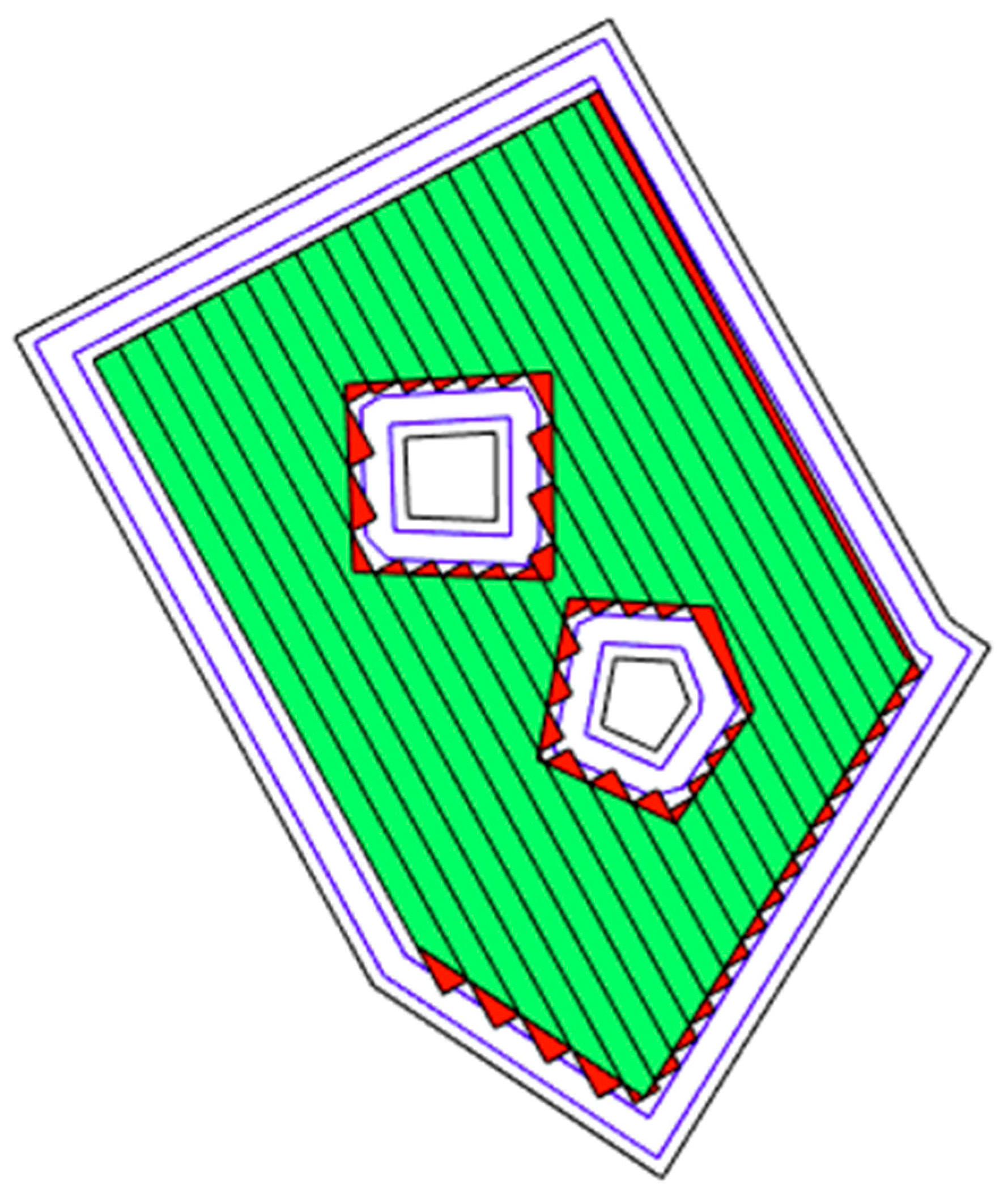
2.3.5. Overlapped Area Quantification

Overlapped area parts, $o$, produced by each row $\mathrm{R}$ can be computed by using the subtraction operator $\mathsf{\Delta }\left(\mathrm{R},F_b\right)$, as illustrated in Figure 11. The total overlapped area ($\mathsf{{\rm O}}$) can be quantified as summation of each individual overlapped area of each row by $O={\sum }_{i=1}^{\tau }|o_i|$.

3. Implementation and Results

The algorithms for generation of geometrical field representations described above were implemented using the JAVA programming language (Oracle Corporation) and executed on a standard computer with a CPU of 3.2 GHz processor and a 4 GB RAM. To demonstrate the functionality of the process, 12 fields with different number of obstacles ranging, from one to six, were selected, representing a range of complexity levels of field shapes. The field shape files were provided by the GIS database from The Ministry of Environment and Food of Denmark. Three types of working width ($w$ = 2 m, 4 m, 6 m) were used. The driving direction for each field is represented by the red marked line suggested by technical staff, as shown in the

Table 3. Computational time for different fields with different number of obstacles.

Field ID	Area (ha)	Shape and Reference Line	Computation Time (s)			Track Type
			$\mathit{w}$ = 2 m	$\mathit{w}$ = 4 m	$\mathit{w}$ = 6 m
1	10.27		0.98	0.73	0.60	Straight
2	22.78		9.63	5.42	2.59	Curved
3	53.06		19.62	6.41	2.72	Curved
4	37.27		14.22	4.83	2.86	Curved
5	15.56		4.82	2.12	0.63	Curved
6	63.27		2.01	1.28	1.12	Straight
7	30.27		24.51	6.81	3.13	Curved
8	37.41		1.78	1.22	1.01	Straight
9	27.58		18.2	6.22	3.62	Curved
10	34.51		1.58	0.97	0.73	Straight
11	74.98		1.57	0.94	0.27	Straight
12	36.3		1.95	1.23	1.01	Straight

. The results of average computation time of the method (as an average of 1000 runs per case) are listed in Table 3.

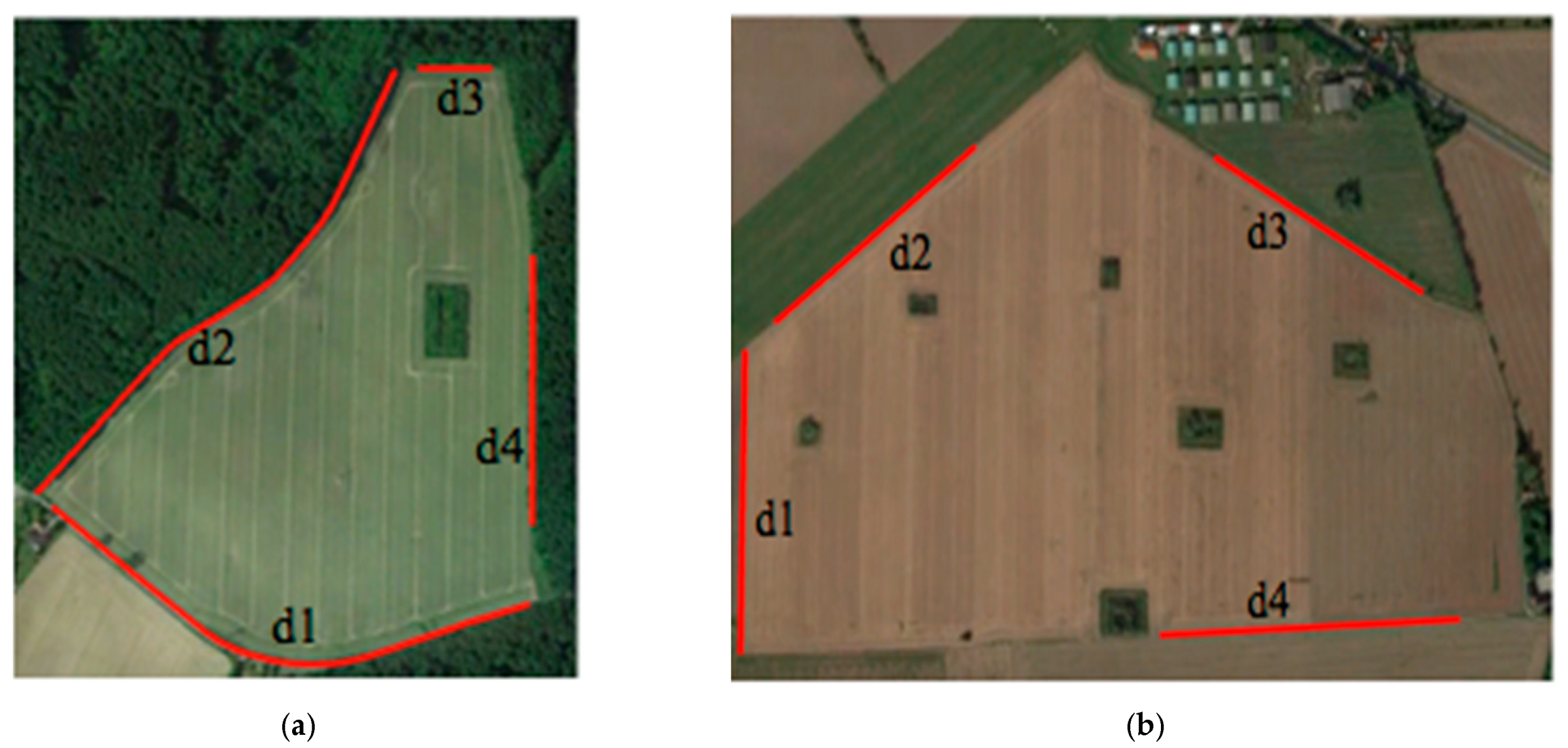
In addition, two scenario studies were carried out to investigate the effect of using different field-work tracks references, directions, and operating widths on the generated metric map. Figure 12 presents the two selected fields (field 2 and field 10 from Table 3) as examples that include both straight and curved field-work tracks.

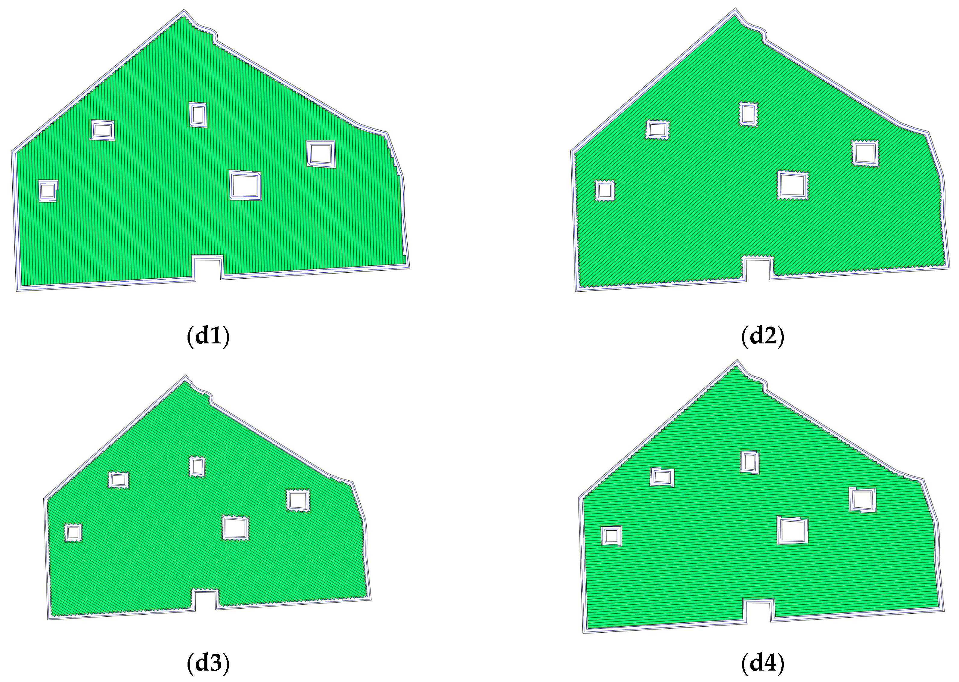
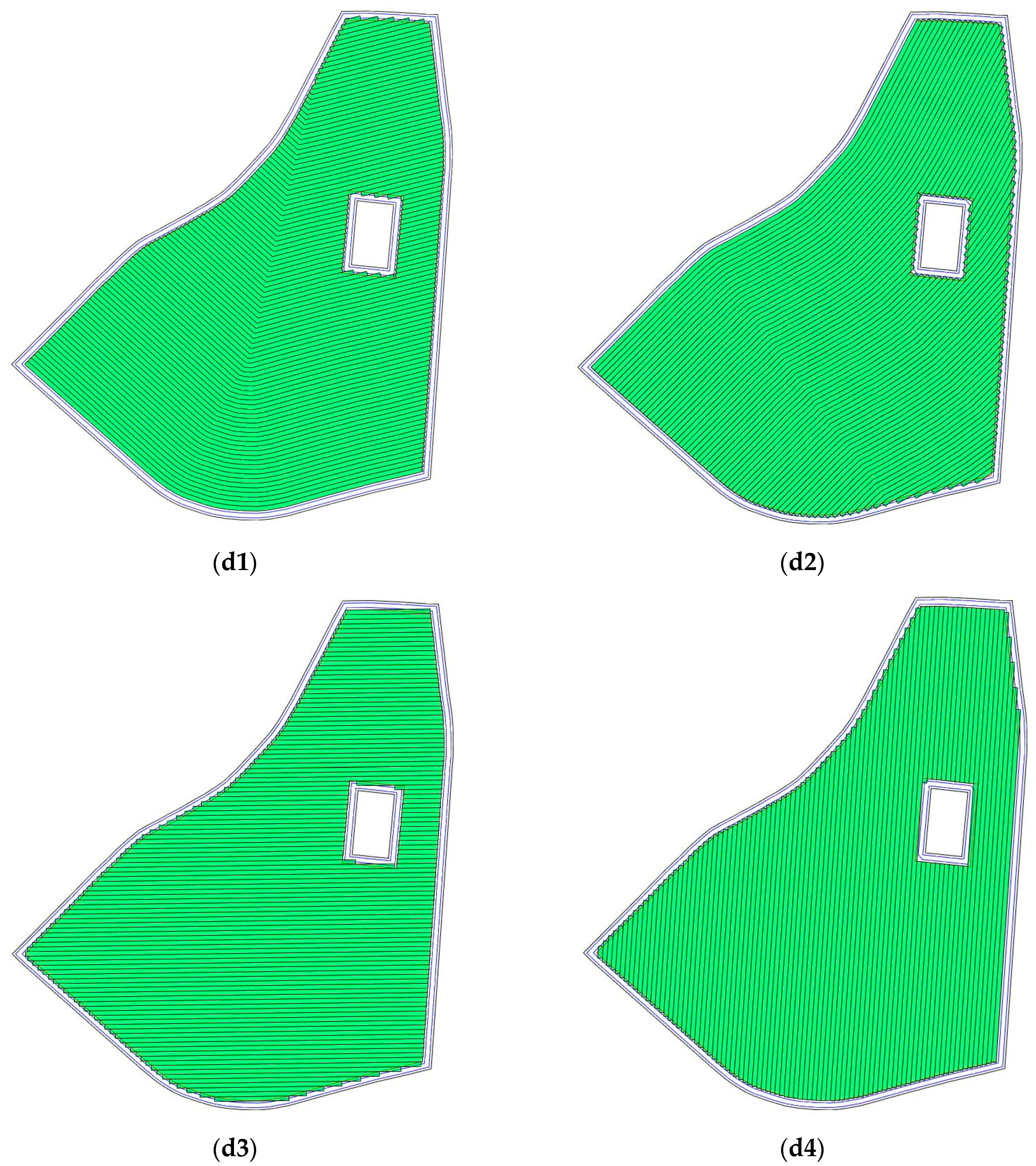
In this scenario, field 10 was selected for test, and four straight reference lines for the generation of straight tracks were used as shown in Figure 13. Field geometrical representations for each direction with 6 m working width are illustrated in

Table 4. The results of field representation when using different straight reference lines.

	$\mathit{w}$ = 4 m				$\mathit{w}$ = 6 m
	d1	d2	d3	d4	d1	d2	d3	d4
Total length of tracks (m)	80,441	80,649	80,787	80,541	51,652	51,799	51,967	51,655
Number of tracks	260	272	262	216	176	184	180	149
Overlapped area (ha)	0.28	0.37	0.42	0.32	0.48	0.57	0.67	0.49

. The tested results are given in Table 4, in which we can see that the driving direction not only determines the number of generated tracks but also determines the size of the overlapped area when the working width is the same. In terms of number of tracks, the maximum difference is up to 56 when comparing driving direction d2 with d4 using working width $\mathit{w}$ = 4 m, while in terms of overlapped area, it can be found that larger working widths lead to larger overlapped areas, which corresponds with conclusions derived by Luck et al. (2010). Additionally, it can be seen that less tracks do not produce less overlapped area, for instance comparing d4 with d1 when working width was 4 m [24].

In this scenario, two curved reference lines and two straight reference lines were used for the generation of tracks for field 2 and field geometrical representations for each direction with 6 m working width are illustrated in Figure 14, and these four reference lines are the possible choices a machine operator will make for field operations. From the results presented in

Table 5. The results of field representation when using both straight and curved reference lines.

	w = 4 m				w = 6 m
	d1 Curved	d2 Curved	d3 Straight	d4 Straight	d1 Curved	d2 Curved	d3 straight	d4 Straight
Total length of tracks (m)	52,027	51,797	52,080	52,068	33,350	33,131	33,358	33,355
Number of tracks	137	178	189	99	91	119	125	99
Overlapped area (ha)	0.20	0.11	0.23	0.33	0.22	0.18	0.34	0.33

, it can be seen that curved tracks resulted in less overlapped area when using the same working width. Among all these setups, the setup that using driving direction d1 and working width $\mathit{w}$ = 6 m might be the most favorable as it yields the fewest number of tracks—implying that less turns are required to cover the entire field, which, consequently might mean less non-working time.

4. Discussion

From the previous two scenario studies, we can see that the presented tool has the potential capability to be used as a decision support system to find, for example, the driving direction that yields the least overlaps (i.e., spraying), or the least number of turns, or can even be used as an input for high-level planning such as path planning [6,7], route planning [8,9,10,11,12,13], and field coverage planning [14,15,16,17,18].

Based on the test results in Table 3, the computational times of the presented method were in the range 0.26–24.51 s for various field shapes, and the area ranged between 10.27 and 74.58 ha. Compared with fields with straight tracks, the map generation for fields with curved tracks requires higher computational times. The average computational time for fields with straight tracks was 1.16 s, while for curved tracks it was 7.69 s. The main reason for higher computational times in the case of curved tracks is that each time a subsequent curved track is constructed, a new curved reference line has to be created, that is, the predecessor curved track. This repetitive process consumes a large percentage of the overall computational time.

The low computational times of the proposed method—in the level of seconds—provides the potential for real-time implementation in agricultural machine navigation systems, precision application tools (e.g., automatic boom section control for spraying), autonomous robots. The importance of a real-time map generation is derived from a number of reasons:

• Not all information about field shapes is often available, so the operator has to drive around the field and obstacles boundaries to acquire the path coordinates, and so the map generation process has to take place on-site.
• The field metric map should be generated based on the effective working width instead of the specified working width which in many cases the operator must adjust to field conditions.
• Factors also such as soil condition in terms of moisture content also affects field shapes and thus affecting the field representation scheme. That might be the case, when, for example, a water area inside the field resulting from rain constitutes an operational obstacle for the proposed method and would require a new field representation to be generated in real-time, on site, for the remainder of the field operation.

The presented tool brings a number of advancements to the process of generating a metric map for arable farming field operations. These advancements include the real-time generation feature, the potential to deal with multiple-obstacle areas, and the reduction in the overlapped area. However, for considering this approach as “complete”, a number of limitations still hold. These limitations include:

• Regarding infield obstacles, the proposed method does not handle cases such as two obstacles in close proximity. These types of obstacles, from the operational point of view, should be considered as one obstacle. Furthermore, cases of small obstacles (e.g., trees, electricity pylons, etc.) that cause a local deviation from the designed track are not taken into account. The categorization of the obstacles depending on the driving direction, working width, the shape of field, size and location of obstacle [18] is an important step in the map generation since it affects the accuracy and feasibility of the generated field representation scheme.
• In the case of curved tracks, each track consists of sequentially connected line segments. There are cases where it is not feasible for an agricultural machine to perform a sharp turn between two line segments due to operational limitations on the maximum turning curvature. Therefore, there is the need for the implementation of curved polyline smoothing algorithms to generate an easier steerable path for agricultural machines [12].
• As part of the tool, the machine operator has to set the value of the number of headland passes manually for generation of the required headland space. It might be difficult for the user to determine an appropriate value due to the fact that the headland space depends on a number of factors such as field shapes, field condition, machine’s kinematic features and so on. Therefore, an algorithm or model should be developed for this tool to improve the reliability of the field representation.
• This tool needs further elaboration so that the user can interactively divide the field into subfields, where each subfield can have its own driving direction.

5. Conclusions

In this paper, a new approach for a metric map generation for autonomous field operations was developed. The generated map consists of either straight or curved field-work tracks for any complexity level of fields in terms of the shape and number of in-field obstacles. According to the test results on 12 selected fields with different numbers of obstacles and diverse shapes, the computational times were in the range of 0.26–24.51 s demonstrating that it is feasible for real-time implementation.

The proposed approach can be deployed for navigation-aiding system for agricultural machinery or as part of the high-level control of autonomous field machines. However, this tool still needs further elaboration in terms of extending with the capability of supporting field subdivision, automatic process for obstacles categorization, automatic determination of headland space, and smooth curve tracks generation.

References

- Sørensen, C.G.; Pesonen, L.; Bochtis, D.D.; Vougioukas, S.G.; Suomi, P. Functional requirements for a future farm management information system. Comput. Electron. Agric. 2011, 76, 266–276. [Google Scholar] [CrossRef]
- Angelopoulou, T.; Tziolas, N.; Balafoutis, A.; Zalidis, G.; Bochtis, D. Remote Sensing Techniques for Soil Organic Carbon Estimation: A Review. Remote Sens. 2019, 11, 676. [Google Scholar] [CrossRef] [Green Version]
- Freidenreich, A.; Barraza, G.; Jayachandran, K.; Khoddamzadeh, A.A. Precision Agriculture Application for Sustainable Nitrogen Management of Justicia brandegeana Using Optical Sensor Technology. Agriculture 2019, 9, 98. [Google Scholar] [CrossRef] [Green Version]
- Liakos, K.; Busato, P.; Moshou, D.; Pearson, S.; Bochtis, D. Machine Learning in Agriculture: A Review. Sensors 2018, 18, 2674. [Google Scholar] [CrossRef] [PubMed] [Green Version]
- Marino, S.; Alvino, A. Detection of Spatial and Temporal Variability of Wheat Cultivars by High-Resolution Vegetation Indices. Agronomy 2019, 9, 226. [Google Scholar] [CrossRef] [Green Version]
- Bochtis, D.D.; Sørensen, C.G.; Vougioukas, S.G. Path planning for in-field navigation-aiding of service units. Comput. Electron. Agric. 2010, 74, 80–90. [Google Scholar] [CrossRef]
- Jensen, M.A.F.; Bochtis, D.; Sorensen, C.G.; Blas, M.R.; Lykkegaard, K.L. In-field and inter-field path planning for agricultural transport units. Comput. Ind. Eng. 2012, 63, 1054–1061. [Google Scholar] [CrossRef]
- Bochtis, D.; Griepentrog, H.W.; Vougioukas, S.; Busato, P.; Berruto, R.; Zhou, K. Route planning for orchard operations. Comput. Electron. Agric. 2015, 113, 51–60. [Google Scholar] [CrossRef]
- Bochtis, D.D.; Vougioukas, S.G. Minimising the non-working distance travelled by machines operating in a headland field pattern. Biosyst. Eng. 2008, 101, 1–12. [Google Scholar] [CrossRef]
- Conesa-Muñoz, J.; Bengochea-Guevara, J.M.; Andujar, D.; Ribeiro, A. Route planning for agricultural tasks: A general approach for fleets of autonomous vehicles in site-specific herbicide applications. Comput. Electron. Agric. 2016, 127, 204–220. [Google Scholar] [CrossRef]
- Hameed, I.A.; Bochtis, D.D.; Sorensen, C.G. Driving angle and track sequence optimization for operational path planning using genetic algorithms. Appl. Eng. Agric. 2011, 27, 1077–1086. [Google Scholar] [CrossRef]
- Spekken, M.; de Bruin, S.; Molin, J.P.; Sparovek, G. Planning machine paths and row crop patterns on steep surfaces to minimize soil erosion. Comput. Electron. Agric. 2016, 124, 194–210. [Google Scholar] [CrossRef]
- Zhou, K.; Bochtis, D. Route Planning For Capacitated Agricultural Machines Based On Ant Colony Algorithms. In Proceedings of the 7th International Conference on Information and Communication Technologies in Agriculture, Food and Environment, Kavala, Greece, 17–20 September 2015; pp. 163–173. [Google Scholar]
- Edwards, G.; Jensen, M.A.F.; Bochtis, D.D. Coverage planning for capacitated field operations under spatial variability. Int. J. Sustain. Agric. Manag. Inform. 2015, 1, 120–129. [Google Scholar] [CrossRef]
- Jin, J.; Tang, L. Coverage path planning on three-dimensional terrain for arable farming. J. Field Robot. 2011, 28, 424–440. [Google Scholar] [CrossRef]
- Jin, J.; Tang, L. Optimal coverage path planning for arable farming on 2D surfaces. Trans. ASAE 2010, 53, 283–295. [Google Scholar] [CrossRef]
- Oksanen, T.; Visala, A. Coverage path planning algorithms for agricultural field machines. J. Field Robot. 2009, 26, 651–668. [Google Scholar] [CrossRef]
- Zhou, K.; Leck Jensen, A.; Sørensen, C.G.; Busato, P.; Bothtis, D.D. Agricultural operations planning in fields with multiple obstacle areas. Comput. Electron. Agric. 2014, 109, 12–22. [Google Scholar] [CrossRef]
- Palmer, R.J.; Wild, D.; Runtz, K. Improving the Efficiency of Field Operations. Biosyst. Eng. 2003, 84, 283–288. [Google Scholar] [CrossRef]
- Taïx, M.; Souères, P.; Frayssinet, H.; Cordesses, L. Path planning for complete coverage with agricultural machines. Springer Tracts Adv. Robot. 2006, 24, 549–558. [Google Scholar]
- Oksanen, T.; Visala, A. Path Planning Algorithms for Agricultural Machines. Agric. Eng. Int. CIGR J. Sci. Res. Dev. 2007. [Google Scholar]
- Hameed, I.A.; Bochtis, D.D.; Sørensen, C.G.; Nøremark, M. Automated generation of guidance lines for operational field planning. Biosyst. Eng. 2010, 107, 294–306. [Google Scholar] [CrossRef]
- Hameed, I.A.; La Cour-Harbo, A.; Osen, O.L. Side-to-side 3D coverage path planning approach for agricultural robots to minimize skip/overlap areas between swaths. Rob. Auton. Syst. 2016, 76, 36–45. [Google Scholar] [CrossRef]
- Luck, J.D.; Pitla, S.K.; Shearer, S.A.; Mueller, T.G.; Dillon, C.R.; Fulton, J.P.; Higgins, S.F. Potential for pesticide and nutrient savings via map-based automatic boom section control of spray nozzles. Comput. Electron. Agric. 2010, 70, 19–26. [Google Scholar] [CrossRef]
Figure 1.
Tracks are represented by red lines and green areas are the covered areas by following the designated tracks. In (a) there are uncovered areas (yellow); in order to cover these areas, the tracks have to be extended (b).
Figure 2.
Examples of a ring (a) and a polygon made up of rings (b).
Figure 3.
Example of an envelope of a polygon. This is the minimum bounding envelope.
Figure 4.
Buffer polygons (green) with offset distance , where is either a straight line segment (a) or a polyline (b).
Figure 5.
Illustrated example of operator projection (a) and point union (b).
Figure 6.
Headland area consisting of rings inside the field and outside the obstacles. Black rings are field and obstacle boundaries, blue rings are headland passes and red rings are the resultant headland area boundaries.
Figure 7.
The bounding envelope of the field is covered by a set of straight lines that are parallel to the reference line l.
Figure 8.
Generation of polygons from initial tracks for three case steps. (a) generate buffer polygon using operator for an initial track ; (b) find as the intersection of and inner field border ; (c) obtain the subtracted area using operator .
Figure 9.
(a) The (blue) projection points of corresponding (red) initial points; (b) The final tracks and corresponding rows; (c) The generated field representation.
Figure 10.
The individual steps of generation of the first curved track.
Figure 11.
An illustration of generated overlapped area (red area) for each row.
Figure 12.
The selected fields 2 (a) and 10 (b) (presented also in Table 3) and the selected direction reference lines (red marked lines) used in the scenario tests.
Figure 13.
Field geometrical representations for direction (d1,d2,d3,d4) with 6 m working width.
Figure 14.