Decision Support Tool for Operational Planning of Field Operations


1
Research & Advanced Engineering, AGCO A/S, 8930 Randers, Denmark
2
Department of Engineering, Aarhus University, 8000 Aarhus, Denmark
*
Author to whom correspondence should be addressed.
Agronomy 2020, 10(2), 229; https://0-doi-org.brum.beds.ac.uk/10.3390/agronomy10020229
Submission received: 14 December 2019
/
Revised: 22 January 2020
/
Accepted: 27 January 2020
/
Published: 4 February 2020
(This article belongs to the Special Issue Agricultural Route Planning and Feasibility)
Abstract
:Precision Farming (PF) and Controlled Traffic Farming (CTF) are well known concepts within agriculture, but the adoption rate of these practices by farmers is still very low, because farmers lack the needed skills or fail to see the benefits of using these practices. If farmers want to reap the full benefits, operational planning must be carried out in advance for the entire crop cycle, before the crop season begins. However, operational planning across the entire crop cycle is a non-trivial task, since the efficiency of each operation is determined by a range of selected operational features (e.g., wayline direction, operational speed, vehicle capacity, wayline sequence, and turn type). To that end, we present, in this paper, an application that can support farmers with operational planning of field operations with CTF, by automating the process. It provides the farmer with an overview of all his field operations, and acts as a decision support tool during the operational planning process. The application allows farmers to store and manage field and equipment information, which is used as input, when setting up CTF and generating way lines and route plans for the individual fields. One of the key benefits of the application is the provided comparison feature, where farmers can compare alternative solutions, based on Key Performance Indicators (KPIs). Results from an example field, for operations with different machine setups, are presented to illustrate how KPIs and visualisations can support farmers during the decision process.
1. Introduction
The world population is growing exponentially and is expected to reach 9.7 billion people by 2050 [1]. This corresponds to an increase in the annual demand for animal protein by 455 million metric tonnes [2]. In order to keep up with the increasing demands, efficiency optimisation of the agricultural sector is paramount. Well-known concepts which can improve efficiency within arable farming is precision farming (PF) and controlled traffic farming (CTF). Common to both is that they not only require investments, but also more knowledge, training, and planning by the farmer.
Field operational planning, in particular, is important when adopting PF and CTF technologies. The goal of operational planning is to optimise the efficiency of field operations, by reducing input costs, while increasing output value. Reduction of input costs can be achieved by optimising input resources through for instance auto steering and section control systems, which reduce overlapped area, and thereby save input goods (seeds, pesticides, etc.), fuel, time, and labour. Proper route planning can additionally reduce fuel, time, and labour cost as the total route length can be minimised through optimisation. Increase in output value can arise from variable rate application systems and minimisation of soil compaction, as these will generally increase yields.
Various algorithms and methods of field operation planning were developed, which mainly solve two distinct tasks: field partitioning and route planning. Field partitioning involves the generation of three types of geometric entities: in-field waylines (straight or curved), headland passes, and turns between waylines and headland passes. Several methods were developed, which are capable of dealing with either two- or three-dimensional field models, with or without obstacle areas [3,4,5,6,7,8,9].
Many route planning algorithms are based on optimisation algorithms which calculate the optimal way to traverse the entities defined in the field partition. These algorithms take into account the operational constraints (e.g., capacity, kinematics) of the involved vehicles, while optimising one or more criteria, such as reducing non-working distance [10,11,12,13,14,15], total operational time [16], consumed energy [17] or soil compaction [18]. Furthermore, some of these algorithms and methods were integrated in commercial field operation management systems to help farmers make better decisions. These commercial tools include LACOS-fieldplanner [19], CLAAS field route optimisation [20], Next Farming field partitioning [21], and IntelliPaths [22] for route planning.
In this paper, we present a decision support tool, which can aid the farmer in the operational planning process. The tool allows the farmer to setup and manage field and equipment information, which is used as input during the operational planning. It enables the farmer to generate way lines, including setting up CTF for a non-uniform vehicle fleet, and to optimise route plans for all operations during the crop cycle. It also enables a quantitative comparison of different operational plans, by calculating KPIs, such as operation time, field efficiency, and fuel consumption. Finally, a qualitative evaluation of the generated route plans is enabled by the tool’s simulation and visualisation capabilities.
2. Materials and Methods
Operational planning is focused on determining the best possible operational plan for performing a given field operation. The input parameters, including field and equipment information, are often known in advance, as they are based on the farmers existing resources. The two sections below describe how and what data is managed in the tool. Next is a description of the steps of the operational planning process, and how these are supported by the presented tool.
2.1. Equipment Management
The tool provides an easy and intuitive way of setting up and maintaining an up-to-date overview of a users equipment (vehicles and implements). Equipment parameters relevant for operational planning include:
- Manufacturer: Optional, used for identifying the machine.
- Model: Optional, used for identifying the machine.
- Year: Optional, used for identifying the machine.
- Resource type: Type of machine, e.g., tractor, sprayer, harvester, etc.
- Turning radius: The minimum possible turning radius for the machine.
- Driving speeds: Estimated in-field driving speed during operation, transport, and turnings.
- Working width: The effective working width of an implement
- Storage capacity: The volumetric size of the storage container on a machine
- Unloading rate: The unloading flow rate of e.g., a combine harvester
- Loading rate: The loading flow rate of e.g., a sprayer
- Hourly cost: The estimated hourly cost, including fuel, maintenance and labour.
2.2. Field Management
Field information can either be imported into the tool through standardised formats, such as Shapefile [23], or created directly in the tool. The following information, for each field, is needed in the operational planning process:
- Field name: Unique field name to identify a field
- Field boundary: A list of geometric points that mark the field boundary.
- Access points: A set of geometric points that mark where the field can be entered.
- Crop row direction: Two geometric points marking the crop row direction of the field (Optional).
- Headland width: The width of the headland area (Optional).
- Size: The field size (calculated based on the field boundary).
2.3. Operational Planning
Operational planning is focussed on determining how to optimise work in the field, both in terms of reducing costs and improving yields. This is done for all field operations in the cropping cycle.
The operational planning process consists of three major tasks: (1) Field partitioning, (2) Route generation, and (3) Evaluation. Field partitioning refers to the process of generating waylines and possible turning manoeuvres for a given field. Route generation consist of generating optimised routes for the vehicles involved in a specific operation. The primary objective of the evaluation is to consider and compare alternative planning solutions, in order to find the solution(s) that provides highest value to the user.
We define an operational plan for a single field operation on one field, as a plan configuration and a corresponding plan solution, which consists of a field partition, optimised routes, and a set of KPIs. A plan configuration consists of the following information:
- Field information: Information for a single field as defined in Section 2.2.
- Equipment information: A list of equipment to be used in the plan, as defined in Section 2.1.
- Operation settings: Settings for the specific operation (varies based on operation type):
- Operation type: The type of operation
- Use of access point: Which access points should be used.
- Application parameters: Application product, rate, cost, and loading strategy.
- Harvest parameters: Crop type, yield estimates, and unload strategy.
2.3.1. Field Partitioning
Given a plan configuration with field and equipment information, a partition can be generated. The partitioning consists of four steps: (1) Divide the field into headland and primary area, (2) Generate smooth headland waylines, (3) Generate waylines for the primary area, (4) Generate feasible turns.
If the headland width is specified in the configuration this is used in step 1, to divide the field. Otherwise the tool calculates the minimum feasible headland width, based on the working width and the turning radius of the machine. Next, the headland waylines are generated (see example in Figure 2).
In step 3, the waylines for the primary area are generated, based on the crop row direction and the working width of the machine. If the crop row direction is not specified, the tool will automatically calculate the most optimal direction. This optimisation is similar to the method presented by Hameed et al. [24], but minimises both the number of waylines (and thereby headland turns) and overlapped area. Finally, all feasible turns between waylines are calculated along with a set of KPIs.
The output of a field partitioning is a graph-like structure, which is used for route generation. In case a farmer is not interested in routes, it is possible to export the waylines, such that these can be imported into auto steering systems.
Controlled Traffic Farming
Ideally, when practising CTF, all vehicles and implements should have identical working widths, axle widths and wheel sizes, such that all machines in all operations throughout the crop cycle could use the exact same wheel tracks. However, this is seldom the case in a conventional farm, if not even impossible, due too the available commercial equipment. Instead, we suggest a “CTF light” approach, where waylines for all operations in the crop cycle are aligned as good as possible, considering the available equipment.
As an example, consider the equipment listed in Table 1, which can be used for three operations: ripping, spraying, and harvesting (6, 12, and 24 m working widths). When setting up CTF, one operation is selected as the highest priority, in this case spraying. First the partition for spraying is generated. Next, one of the waylines from the spraying partition is used as the base wayline when creating/propagating waylines for the ripping and harvesting operations. This makes sure that the waylines from all three partitions are aligned as good as possible.
In Figure 3, the combined set of waylines for all three operations are shown, both when using CTF and not. The difference is clearly visible, and in Figure 4 the combined track area of all three operations are shown. For simplicity we assume identical axle and tire configuration on all vehicles: Axle width = 2 m and tire width = 0.65 m. In this simple case with only three operations, the tracked area is reduced with 8.5%.
2.3.2. Route Generation
Waylines and feasible turns are generated in the field partition, but it does not provide any advise on how or in which order to traverse these. Especially for capacitated operations, such as seeding, spraying, and harvesting operations, time and cost can be reduced by optimising how to traverse the waylines, and where and when to load or unload machines. This optimisation is performed in the route generation process, where routes for each machine are created. The routes contain information about where to go, and what to do at all times. An example of a route driving pattern for a harvester is shown in Figure 5. In the application, the machine movements and actions can be simulated, such that the user can see exactly when actions, such as unloading, need to take place.
2.3.3. Evaluation and Comparison
A range of KPIs are calculated as part of field partitioning and route generation, see Table 2. These KPIs along with the visualisations are the only way for the farmer to evaluate the calculated plan solutions. Some of the KPIs are calculated for the complete operation, as well as for the individual machines. This is relevant when evaluating plans with multiple machines, to see if a single machine is imposing a bottleneck in the system, or if some machines are idling too much.
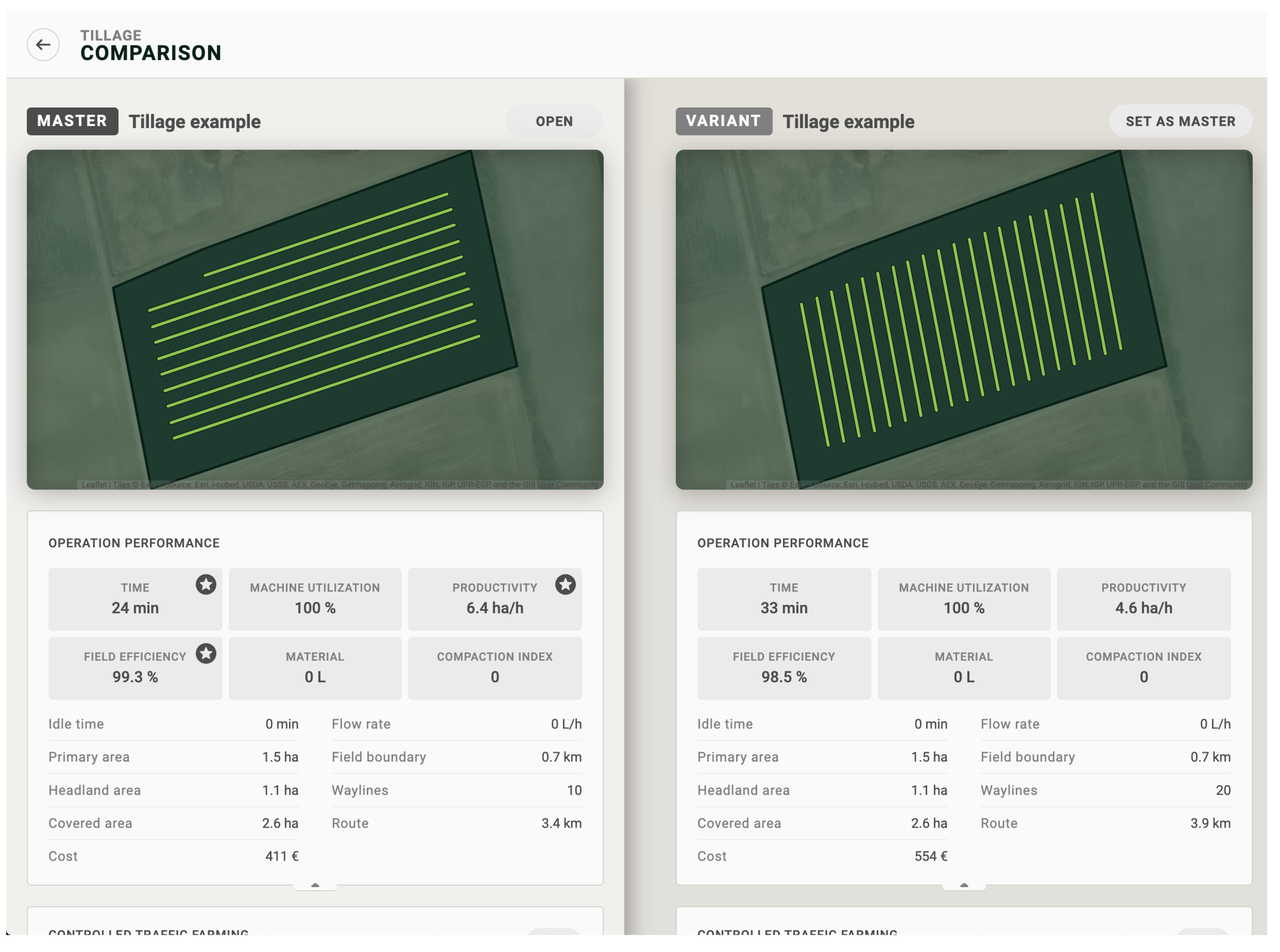
The KPIs are especially valuable, when exploring alternative plan solutions, as they enable a quantitative comparison that cannot be made based on visualisation alone. The exploration process should aid the user, when considering non-trivial questions, such as whether to use CTF or not, and which CTF setup performs best, given the farmers current equipments. One could also explore what the impact is of using multiple or alternative machines, or alternative loading strategy or other input parameters. Comparison of potential plan solutions is made easy in the application, by representing the KPIs in a structured way, and highlighting the plan variants with best-scoring KPIs, see Figure 6 for a comparison of two alternative tillage plan configurations.
3. Results
Based on the test field and equipment examples defined in Section 2, we present results for two concerns: (1) Is it beneficial to use CTF for this setup? and (2) Is it beneficial to use more than one machine in each field operation?
3.1. CTF vs. Non-CTF
The question of whether to use CTF is a complex matter, as the cost effectiveness can be difficult to measure [25]. One of the key reasons of using CTF is to minimise the tracked area of the field, as each track potentially causes soil compaction and crop damage, and thereby reduces yield.
In the ideal CTF setup all equipment have the same working width, and the same axle and tire configuration, but this is seldom the case in a conventional farm. With our CTF light approach, farmers can evaluate how CTF plans will perform with their current equipment.
In order to give an idea of how our tool can provide farmers with decision support about using CTF or not, a comparison was made for the test field (Figure 1) and the three operations: ripping, spraying and harvesting. For the CTF configuration, the spraying operation is prioritised highest. An extract of KPIs, for these plans, is shown in Table 3. As expected, the total tracked area across operations is reduced (from 40.2% to 31.7%), when using CTF compared to the conventional non-CTF approach. The downside of using CTF is reflected in the other listed KPIs. The total overlapped area is increased with 7.5%, and the total route time is increased with less than 2 min (less than 2.5%). Please note that the overlapped area is calculated as a sum of all three operations. The overlapped area for the sprayer remains constant, while ripping and harvest increases. This is an interesting observation, as overlapped area is mainly a concern for application operations (seeding, spraying, fertilising, etc.), because overlap means higher cost for the applied goods. For ripping and harvest, overlapped area is insignificant, as it does not add extra costs, except the slightly longer route distance. One could similarly argue that overlapped area is also insignificant for application operations, if the equipment is equipped with section control.
As stated previously, our application does not dictate what a farmer should do in this situation, nor does it tell what is the optimal solution, as it most likely depends on other factors as well. We leave it up to the farmer to decide if the reduction of tracked area is significant enough to spend the extra time and effort on implementing CTF.
3.2. Multiple Machines
With the same field and equipment setup from previously, we evaluate what happens, when multiple identical machines are to carry out the field operations in cooperation. Specifically, we simulate all three operations with one, two, and three machines. Table 4 shows an extract of KPIs for all these simulations, while Figure 7 shows the routes for the ripper operation with three machines. As expected, the operation time is decreasing, when using more machines. However, the time is not exactly inversely proportional to the number of machines used. Hence, changing from one to two machines does not half the operation time. One reason is that the total route distance for all machines increase slightly, as more machines are added. Another reason is that idle time can occur in some cases, when the machines carry out the headland part of the field, in order to avoid collisions. This is also reflected in the productivity and field efficiency KPIs.
Note for the sprayer operation with three machines, the application generates a solution, where only two machines are used. This happens because the field is so small that it does not improve the operation performance to add a third machine.
4. Discussion
One of the challenges, when optimising and automating the operational planning process, is to define what an optimal solution is. Often the objective has multiple criteria, such as reducing cost, minimising operation duration, increasing yields by minimising tracked area, or others. Unfortunately these criteria are often conflicting, which is why the application is developed as a decision support tool, rather than an application that can make all decisions autonomously.
One example of a trade-off between criteria is evident when generating turn manoeuvres. A minimum turn with shortest distance and minimum turning radius is optimum from an algorithmic standpoint, but will feel very uncomfortable for the driver and causes more stress on the equipment, which eventually means higher maintenance and repair costs. Another issue with turn manoeuvres is coverage in the headland area. If turns with reversing is not permitted, there will be uncovered area in the headland corners (see Figure 7). This is accepted by some farmers, while others find it unacceptable. This comes down to a trade-off between coverage and efficiency.
Compared to other existing tools, we believe that this tool provides more (advanced) features in a simpler way, while giving a better understanding of the process and the results. Simplicity originates from the user experience, since all decision variables in the tool have default values or are optimised automatically, unless the user overrides these settings. In the simplest planning flow, the user only needs to pick a field, a machine, an operation type, and a plan name as input, and then the tool generates a complete route plan, including visualisations and KPIs. Comparison of plans are similarly simplified, as the user only has to create a variant of an existing plan, and change the desired input parameter(s), and can following access the comparison view (see Figure 6 for an example).
The CTF light features, including aligning waylines across different operations and calculating tracked area, are to our knowledge not found in any other available tool. Neither is the simulation feature, which give users a better understanding of the calculated results. The calculated KPIs are very valuable when comparing alternative solutions, but one key concern when developing such a tool is user acceptance. If the user does not trust the system and the results, it will not be used. Therefore, the visualisation and simulation features are crucial, as the results are otherwise very difficult to understand, even when using KPIs. Thus, the tool offers a way to evaluate the generated result both quantitatively, be means of KPIs, and qualitatively by means of the visualisation and simulation.
5. Concluding Remarks
In this paper, we presented a decision support tool that enable farmers to make well founded decisions about their operational planning of field operations. Compared to existing commercially available tools, this is not targeted agronomy/software experts, but the average farmer who is not a software expert. The tool requires practically no prior training to use, and can assist farmers with complex matters, such as setting up CTF or making quantitative comparisons of alternative plan solutions. Furthermore, it also supports generation of optimised route plans for multi-vehicle field operations, which minimises the total driving distance in the field and thereby lowering costs and soil compaction.
We envision that this tool will be a critical enabler to increase the adoption rate of CTF among farmers, as the planning process becomes so simple that every farmer will be able to do it without the need for expensive expert consultants. In the future, also other precision farming practices, such as variable rate application, should be supported in the tool, with a similar focus on simplicity and usability.
Author Contributions
Methodology, R.S.N., K.Z.; software, R.S.N., K.Z.; writing—original draft preparation, R.S.N., K.Z.; writing—review and editing, R.S.N., K.Z. All authors have read and agreed to the published version of the manuscript.
Funding
This research was funded by The Danish Innovation Foundation grant number 7038-00249B.
Conflicts of Interest
The authors declare no conflict of interest.
References
- Nations, U. World Population Prospects 2019: Highlights. U. N. Dep. Econ. Soc. Aff. Popul. Div. 2019. [Google Scholar] [CrossRef]
- Available online: https://www.wsj.com/articles/how-to-satisfy-the-worlds-surging-appetite-for-meat-1449238059 (accessed on 14 December 2019).
- Hameed, I.; Bochtis, D.; Sørensen, C.; Nøremark, M. Automated generation of guidance lines for operational field planning. Biosyst. Eng. 2010, 107, 294–306. [Google Scholar] [CrossRef]
- Hameed, I.; Bochtis, D.; Sørensen, C.G.; Jensen, A.L.; Larsen, R. Optimized driving direction based on a three-dimensional field representation. Comput. Electron. Agric. 2013, 91, 145–153. [Google Scholar] [CrossRef]
- Oksanen, T.; Visala, A. Coverage path planning algorithms for agricultural field machines. J. Field Robot. 2009, 26, 651–668. [Google Scholar] [CrossRef]
- Jin, J.; Tang, L. Coverage path planning on three-dimensional terrain for arable farming. J. Field Robot. 2011, 28, 424–440. [Google Scholar] [CrossRef]
- Zhou, K.; Jensen, A.L.; Sørensen, C.G.; Busato, P.; Bothtis, D. Agricultural operations planning in fields with multiple obstacle areas. Comput. Electron. Agric. 2014, 109, 12–22. [Google Scholar] [CrossRef]
- Sabelhaus, D.; Röben, F.; zu Helligen, L.P.M.; Lammers, P.S. Using continuous-curvature paths to generate feasible headland turn manoeuvres. Biosyst. Eng. 2013, 116, 399–409. [Google Scholar] [CrossRef]
- Backman, J.; Piirainen, P.; Oksanen, T. Smooth turning path generation for agricultural vehicles in headlands. Biosyst. Eng. 2015, 139, 76–86. [Google Scholar] [CrossRef]
- Bochtis, D.; Griepentrog, H.W.; Vougioukas, S.; Busato, P.; Berruto, R.; Zhou, K. Route planning for orchard operations. Comput. Electron. Agric. 2015, 113, 51–60. [Google Scholar] [CrossRef]
- Edwards, G.T.; Hinge, J.; Skou-Nielsen, N.; Villa-Henriksen, A.; Sørensen, C.A.G.; Green, O. Route planning evaluation of a prototype optimised infield route planner for neutral material flow agricultural operations. Biosyst. Eng. 2017, 153, 149–157. [Google Scholar] [CrossRef]
- Conesa-Muñoz, J.; Pajares, G.; Ribeiro, A. Mix-opt: A new route operator for optimal coverage path planning for a fleet in an agricultural environment. Expert Syst. Appl. 2016, 54, 364–378. [Google Scholar] [CrossRef]
- Utamima, A.; Reiners, T.; Ansaripoor, A.H. Optimisation of agricultural routing planning in field logistics with Evolutionary Hybrid Neighbourhood Search. Biosyst. Eng. 2019, 184, 166–180. [Google Scholar] [CrossRef]
- Seyyedhasani, H.; Dvorak, J.S.; Roemmele, E. Routing algorithm selection for field coverage planning based on field shape and fleet size. Comput. Electron. Agric. 2019, 156, 523–529. [Google Scholar] [CrossRef]
- Jensen, M.F.; Bochtis, D.; Sørensen, C.G. Coverage planning for capacitated field operations, part II: Optimisation. Biosyst. Eng. 2015, 139, 149–164. [Google Scholar] [CrossRef]
- Spekken, M.; Bruin, S. Optimized Routing on Agricultural Fields by Minimizing Maneuvering and Servicing Time; Precision Agriculture, Springer Science+Business Media: New York, NY, USA, 2013; Volume 14, pp. 224–244. [Google Scholar]
- Rodias, E.; Berruto, R.; Busato, P.; Bochtis, D.; Sørensen, C.; Zhou, K. Energy savings from optimised in-field route planning for agricultural machinery. Sustainability 2017, 9, 1956. [Google Scholar] [CrossRef] [Green Version]
- Bochtis, D.D.; Sørensen, C.G.; Green, O. A DSS for planning of soil-sensitive field operations. Decis. Support Syst. 2012, 53, 66–75. [Google Scholar] [CrossRef]
- LACOS Fieldplanner. Available online: https://www.365farmnet.com/en/farm-management-software/365plus-agricultural-management/precision-farming/lacos-field-planner/ (accessed on 1 December 2019).
- CLAAS Field Route Optimisation. Available online: https://www.365farmnet.com/en/farm-management-software/365plus-agricultural-management/precision-farming/claas-field-route-optimisation/ (accessed on 1 December 2019).
- NEXT Farming. Available online: https://www.nextfarming.com (accessed on 1 December 2019).
- Intellipaths. Available online: http://www.agrointelli.com/intellipaths.html#intellipaths (accessed on 1 December 2019).
- ESRI, U.; PaperdJuly, W. ESRI shapefile technical description. Comput. Stat 1998, 16, 370–371. [Google Scholar]
- Hameed, I.A.; Bochtis, D.; Sorensen, C. Driving angle and track sequence optimization for operational path planning using genetic algorithms. Appl. Eng. Agric. 2011, 27, 1077–1086. [Google Scholar] [CrossRef]
- Chamen, T. Controlled traffic farming–from worldwide research to adoption in Europe and its future prospects. Acta Technol. Agric. 2015, 18, 64–73. [Google Scholar] [CrossRef] [Green Version]
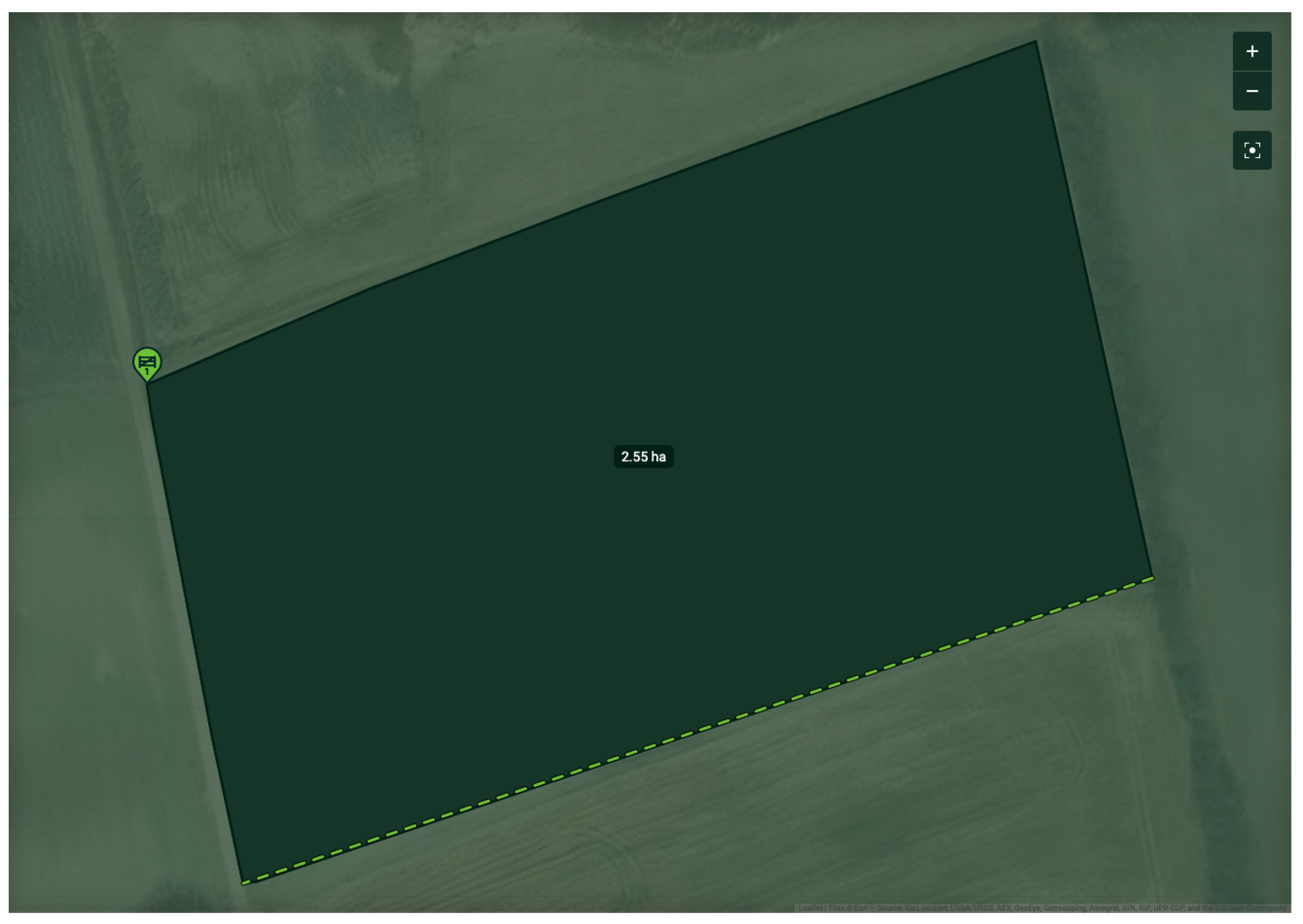
Figure 1.
Example field, showing the field boundary, size, access points (round marker) and crop row direction (dotted line).
Figure 1.
Example field, showing the field boundary, size, access points (round marker) and crop row direction (dotted line).

Figure 2.
Field partitioning example: Generated waylines and possible turnings.

Figure 3.
Controlled traffic farming: Combined set of all waylines across the three operations.

Figure 4.
Controlled traffic farming: Tracked area for all three operations.

Figure 5.
Route plan for a harvest operation.

Figure 6.
Comparison view for different plan configurations for a tillage operation.

Figure 7.
Route plan for a ripper operation with three machines.


Table 1.
Equipment parameters used for the results presented in this paper.
| Type | Turning Radius | Speed | Working Width | Storage Capacity | (Un)Loading Rate | Hourly Cost | ||
|---|---|---|---|---|---|---|---|---|
| Operation | Transport | Turning | ||||||
| Tractor | 6 m | - | 15 km/h | 5 km/h | - | - | - | 100 € |
| Ripper | 7 m | 8 km/h | - | 5 km/h | 6 m | - | - | 0 |
| Sprayer | 6 m | 8 km/h | - | 5 km/h | 24 m | 3300 L | 30 L/s | 0 |
| Harvester | 7 m | 8 km/h | 15 km/h | 5 km/h | 12 m | 12,500 L | 120 L/s | 120 € |
Table 2.
List of calculated KPIs. KPIs marked with an is calculated for each machine and as a total for the complete operation.
Table 2.
List of calculated KPIs. KPIs marked with an is calculated for each machine and as a total for the complete operation.
| Name | Description | Unit |
|---|---|---|
| Waylines | The total number of waylines for a given plan | |
| Covered area | The area of the field, which is covered by the implement | ha |
| Tracked area | The area of the field, which is covered by wheel tracks | % (m) |
| Overlapped area | The area of the field, where coverage overlap occurs | % (m) |
| Operation time | The duration of a field operation | HH:MM:SS (s) |
| Route distance | The distance travelled for a field operation | m |
| Productivity | Area covered pr. hour | ha/h |
| Material | The amount of material applied or collected from the field | t |
| Flow rate | The amount of material applied or collected from the field pr. hour | t/h |
| Loads | The number of unloads/reloads | |
| Cost | The estimated cost of the operation | € |
| Idle time | The time spent idling | HH:MM:SS (s) |
| Machine use | A measure of how much of the time each machine is active. Calculated as: | % |
| Field efficiency | A measure of how efficient a field operation is. Calculated as: , where | % |
Table 3.
Key performance indicators for CTF vs. non-CTF.
| KPI | CTF | Ripping | Spraying | Harvest | Total |
|---|---|---|---|---|---|
| Tracked area | CTF | 22.2% | 6.3% | 11.7% | 31.7% |
| Non-CTF | 22.5% | 6.3% | 11.7% | 40.2% | |
| Overlapped area | CTF | 4.4% | 6.5% | 9.1% | 20% |
| Non-CTF | 2.3% | 6.5% | 3.7% | 12.5% | |
| Operation time (HH:MM:SS) | CTF | 40:14 | 10:53 | 22:35 | 1:13:42 |
| Non-CTF | 39:12 | 10:53 | 21:54 | 1:11:59 | |
| Route distance (km) | CTF | 5.110 | 1.452 | 2.869 | 9.431 |
| Non-CTF | 4.928 | 1.452 | 2.851 | 9.231 |
Table 4.
Key performance indicators for 1 vs. 2 machines.
| KPI | # of Machines | Ripping | Spraying | Harvest |
|---|---|---|---|---|
| Operation time (MM:SS) | 1 | 40:14 | 10:53 | 22:35 |
| 2 | 22:21 | 8:34 | 14:03 | |
| 3 | 18:27 | - | 10:24 | |
| Route distance (km) | 1 | 5.1 | 1.5 | 2.9 |
| 2 | 5.3 | 1.6 | 3.4 | |
| 3 | 5.4 | - | 3.4 | |
| Productivity (ha/h) | 1 | 3.9 | 14.5 | 6.5 |
| 2 | 7 | 19.1 | 10.7 | |
| 3 | 8.5 | - | 14.4 | |
| Cost (€) | 1 | 67 | 19 | 46 |
| 2 | 73 | 22 | 53 | |
| 3 | 81 | - | 52 | |
| Field efficiency | 1 | 98.3% | 93.2% | 95.9% |
| 2 | 94.8% | 91.6% | 90.9% | |
| 3 | 85.5% | - | 90.0% |
© 2020 by the authors. Licensee MDPI, Basel, Switzerland. This article is an open access article distributed under the terms and conditions of the Creative Commons Attribution (CC BY) license (http://creativecommons.org/licenses/by/4.0/).
Share and Cite
MDPI and ACS Style
Nilsson, R.S.; Zhou, K. Decision Support Tool for Operational Planning of Field Operations. Agronomy 2020, 10, 229. https://0-doi-org.brum.beds.ac.uk/10.3390/agronomy10020229
AMA Style
Nilsson RS, Zhou K. Decision Support Tool for Operational Planning of Field Operations. Agronomy. 2020; 10(2):229. https://0-doi-org.brum.beds.ac.uk/10.3390/agronomy10020229
Chicago/Turabian StyleNilsson, René Søndergaard, and Kun Zhou. 2020. "Decision Support Tool for Operational Planning of Field Operations" Agronomy 10, no. 2: 229. https://0-doi-org.brum.beds.ac.uk/10.3390/agronomy10020229
Note that from the first issue of 2016, this journal uses article numbers instead of page numbers. See further details here.