Weed Seed Bank Diversity in Dryland Cereal Fields: Does it Differ Along the Field and Between Fields with Different Landscape Structure?

Abstract

In this work, we aimed to test whether taxonomic diversity and functional diversity and the values of functional traits of the weed seed bank varied across the field, from margins to the core, and between fields embedded in distinct landscape structures. We sampled the seed bank of 47 conventionally managed cereal fields from two Mediterranean regions in Spain. In each field, three positions were selected: Margin, edge and core, and soil properties were measured for each position. Landscape structure was quantified for each field as the percentage of arable land in the surrounding 1 km radius circular sector. Seed bank diversity was characterized at the taxonomic (species richness, exponential Shannon index, and evenness) and functional levels (Rao’s quadratic entropy index and four corner analysis). For functional diversity, eight functional traits related to the whole plant life cycle were considered. Results showed a slight response of increasing taxonomic diversity from the core of the fields to the margins. Functional diversity was extremely low, indicating high similarity among species in terms of functional traits. Species in the seed bank were mostly therophytes, shorter than the crop plants, small seeded, flowering between the herbicide application of late winter and crop harvest, and showed seed dispersal by gravity or wind. This trait syndrome allows persistence in intensively managed arable lands. The similarity between fields in terms of functional diversity of the seed bank and in species traits may suggest that the intensity of management practices was similar across the fields. Moreover, it emphasizes that an increase in landscape heterogeneity, if based on other intensively managed cropping systems, may not be sufficient to augment functional diversity of weed communities. Therefore, in these areas, the seed bank could restore weed taxonomic diversity following changes in management practices, but functional diversity would still remain limited.

1. Introduction

A dramatic diversity loss in arable systems has resulted from agriculture intensification in recent decades. The soil seed bank can function as a reservoir of weed diversity that can serve to restore above-ground diversity in intensively managed agroecosystems. As such, it has been considered indicative of the sustainability of a cropping system [1]. This is because the seed bank encompasses weed seeds from the present and the previous years and, therefore, represents a synthesis of the management practices and the environmental conditions that a field has been subjected to during the years [2]. In this manner, a low diverse weed seed bank, in terms of the number of species, may result from a continuous management regime that has filtered out species. This could be mirrored by a poor diverse seed bank in terms of functional diversity, which can have profound consequences for the functioning of the agroecosystem. First, the remaining weed species would have been those able to cope with the harsh conditions; this is, species with attributes that have allowed them to be competitive for resources and to resist the different disturbances [3]. Second, a lower functional diversity jeopardizes the ability of the weed community to sustain other taxa inhabiting agroecosystems such as arthropods or birds [3,4]. Regardless the management practices the diversity of the weed seed bank could be heterogeneous across the field, because the intensity of the disturbances (i.e., the intensity of the management practices) may vary across the field, being higher at the core than at the edges of the fields, and having the lowest intensity at the margins (i.e., non-cropped strips of spontaneous vegetation surrounding the crop field [5]. In this sense, several works focusing on the emerged weed communities have found higher weed species richness at field edges and margins than at the core of the fields [5,6]. In the case of the seed bank, this pattern could be more accentuated, which could support the idea that field edges and margins are effective refuges for declining weed species [5,7]. Thus, these areas will represent an opportunity for recovering the diversity of the weed communities across the field. Moreover, we argue that not only the management practices determine the diversity of the weed seed bank, but that the structure of the landscape in which a field is embedded could also contribute to differences in the resultant seed bank community. This has been previously found for emerged weed communities. Weed species richness was higher in cereal fields located in landscapes with some proportion of non-cropped habitats or varied agricultural land-uses than in landscapes dominated by arable lands [8,9]. This suggests that different agricultural land uses can lead to distinct weed communities, promoting weed diversity across the landscape, but also that the processes of weed dispersal are of substantial importance in the maintenance of weed populations at a field scale [10,11]. This is despite intensive conventional agricultural practices, weed species could still persist by dispersing from more favorable habitats. Again, this being true provides a chance for enhancing weed diversity at the field scale.

In this work, we aimed to test whether taxonomic diversity, functional diversity, and the values of functional traits of the weed seed bank varied along the field, from margins to the center, and between fields embedded in distinct landscape structures. We focused on Mediterranean cereal fields under conventional management to control for differences in management practices that would have arisen if comparing organic and conventional fields. In addition, focusing on both taxonomic and functional diversity allowed us to analyze changes from a community-based perspective. To complement this approach, functional traits were analyzed to identify those traits that were most associated with shifts in the landscape structure and environmental variation across fields. As we looked at the weed species pool available for recruitment, our experimental approach was intended to quantify the germinating component of the seed bank, i.e., the portion of soil-stored seeds able to germinate along the current crop season. In this way, we avoided the masking effects of post-emergence mortality events, which would hinder the characterization of potential communities based on measuring above-ground vegetation. We hypothesized (a) that the taxonomic and functional diversity of the weed seed bank will decrease along a gradient from the field margins to the core of the field, (b) that the diversity of the weed seed bank will be higher as the adjacent landscape structure is more complex (less arable land), and (c) that specific traits will change at the center of the fields and/or in simple landscapes.

2. Materials and Methods

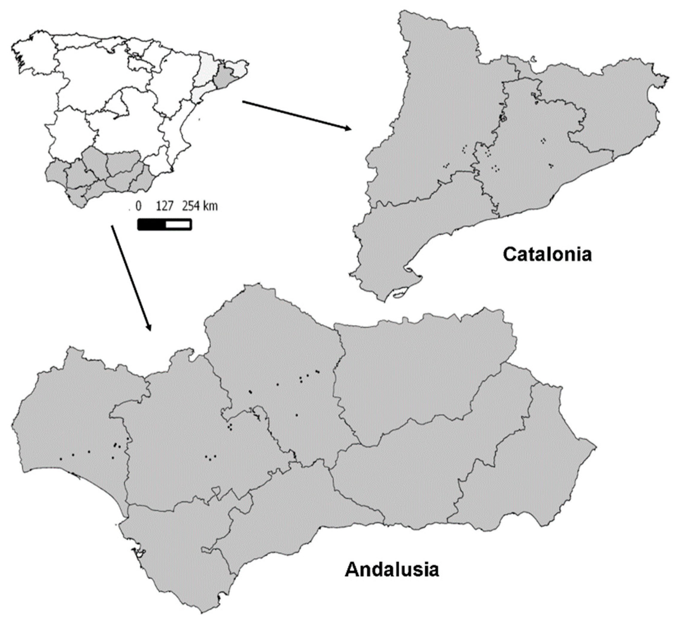
2.1. Study Areas

The study was conducted in 2 areas devoted to cereal crops located in 2 regions, Andalusia and Catalonia, in the south and northeast Spain, respectively (Figure 1). In central Catalonia, the arable land is well intermingled with non-agricultural areas, while in the Gualdalquivir Basin (Andalusia), the arable land is the main land use apart from human settlements. Both areas share a Mediterranean climate, with an average annual temperature of 18.6 °C and 15.5 °C, and mean annual precipitation of 590 and 640 mm in the Guadalquivir Basin and central Catalonia, respectively. In total, 47 conventionally managed cereal fields were sampled; 23 fields in the Guadalquivir Basin and 24 in Central Catalonia. Fields in both areas were managed under short crop sequences, with inorganic fertilization and with the application of herbicides. The fields were selected to represent a gradient of arable land cover, that goes from a matrix habitat dominated by cereal crops to a matrix where other types of crops (e.g., olive) and natural habitats (e.g., forest) predominate.

The soils of the sampled fields were alkaline, with textures varying from clayish to sandy loam. The main land-uses in the 1 km radius circular sector around sampled fields in the Andalusia area were arable land (mean value 61.3%), followed by olive orchards, vineyards, and human settlements. In the Catalonian area, the main land-uses were arable land (75.6%) followed by woodland, other perennial crops, and human settlements.

Table 1. Categories or mean ± standard deviation (SD), minimum and maximum values of the independent variables included in the analyses. Values are separated for the cereal fields sampled in Andalusia (23) and Catalonia (24). Abb. Abbreviation used in the main text.

			Andalusia			Catalonia
Variable	Abb.	Position	Mean ± SD	Min.	Max.	Mean ± SD	Min.	Max.
Organic Nitrogen (%)	N	Margin	0.12 ± 0.01	0.04	0.24	0.19 ± 0.02	0.06	0.40
		Edge	0.10 ± 0.01	0.04	0.17	0.17 ± 0.03	0.09	0.50
		Core	0.09 ± 0.01	0.04	0.15	0.18 ± 0.02	0.07	0.70
Clay (%)	C	Margin	23.90 ± 1.94	10.4	44.2	15.70 ± 0.82	9.00	23.00
		Edge	25.99 ± 2.61	8.20	61.3	17.30 ± 0.73	10.30	22.80
		Core	29.60 ± 2.75	12.00	61.6	18.44 ± 0.88	11.70	27.90
Arable land cover (%)	AL		61.30 ± 34.89	6.00	100	75.60 ± 22.66	25.00	100

shows field characterization in terms of landscape structure and soils.

2.2. Seed Bank Sampling and Seedling Identification

The seed bank sampling was performed during September and October of 2010 and 2011, i.e., immediately before cereal sowing. In each field, 3 positions were delimited: The field margin (uncropped vegetation strip next to the crop), the field edge (the first 5 cultivated meters adjacent to the field margin), and the field core (at least 25 m away from the field margin). These positions reflected potential differences in the disturbance regimes. In every case, the selected field margin was next to a road or a path to avoid the influence of neighboring fields [12]. The selected field edge was adjacent to its margin. In each field, 27 soil samples of 4 cm in diameter and 15 cm depth, or 20 soil samples of 3 cm in diameter and 15 cm depth, were taken per position in Andalusia and Catalonia, respectively. At the margin and at the edge, soil samples were taken in a zigzag manner every 1 m, and at the core position, they were taken every 5 m in a diagonal line towards the field center. For seedling identification, the soil samples were pooled by position resulting in 141 total soil samples (3 field positions × 47 fields). The samples were placed in plastic trays (45 cm × 29 cm × 10 cm) over a thin vermiculite layer covered with an organza cloth, aimed at buffering soil water content fluctuations. The trays were randomly placed on benches in a non-heated greenhouse under natural light conditions, and they were kept moist by regular watering. The position of the trays was randomized every 2 weeks, and soil was carefully mixed every 2 months to favor seed germination and to prevent the growth of mosses. Seedlings were identified, counted, and removed as they emerged, or transplanted for later identification. The census lasted at least 8 months each year, thus covering or surpassing the length of the crop cycle, and finished when there was no further emergence for a period of 2 consecutive weeks [2]. We acknowledge that this procedure, based on emergence counts, does not allow for quantifying full populations of viable seeds in the soil. Rather, our goal was to quantify the germinating component of the seed bank, i.e., the portion of soil-stored seeds able to germinate during the current crop season, as we looked at potential weed species assemblages.

We considered the field position (FP) of the sample: Margin, edge, or core as an indicator of the intensity of the disturbance regime at the field scale. The percentage of arable land (AL) around each sampled field was used as a measure of landscape structure. We obtained the cover of arable land within a circular area of a 1 km radius centered at each field margin, using SIGPAC (Geographic Information System for Agricultural Parcels [13]). We considered that the higher proportion of arable land, the more simplified was the landscape structure.

Finally, we also accounted for the soil chemical and physical structure as this can affect the water storage capacity and the fertility of the soil. In this manner, soil properties can affect weed growth as well as its richness and community composition because species vary in their capacity to germinate and grow under different soil conditions. To do that, simultaneously to the seed bank sampling, 4 soil samples at a depth of 15 cm were taken randomly at each field position (6 kg approx. per field). From each sample, the percentage of sand, silt and clay, organic nitrogen and organic matter, extractable phosphorus, and available potassium were obtained. Organic nitrogen was measured with the Kjeldahl method, assimilable phosphorus was measured with the Olsen method, available potassium and magnesium were measured with the photometric method, and organic matter was determined using the Walkley-Black method. All analyses were performed at Agrifood laboratory of Cordoba (Spain). The correlation among variables was explored to choose the most representative ones. Two of these variables were ultimately selected as putative explanatory variables reflecting physical (percentage clay, thereafter C) and chemical soil properties (organic nitrogen content, thereafter N). Clay was correlated with the percentage of sand (Andalusia: r = −0.73, p < 0.01 and Catalonia r = −0.5, p < 0.01) and Nitrogen was strongly correlated with all the other soil chemical properties (Andalusia: phosphorus, r = 0.47, p < 0.05; organic matter r = 0.9, p < 0.05; potassium r = 0.39, p < 0.05. Catalonia: phosphorus, r = 0.3, p < 0.05; organic matter, r = 0.93, p < 0.05; potassium r = −0.56, p < 0.05).

2.3. Weed Functional Traits

A set of 8 functional traits associated with the vegetative and reproductive phases of the weed life-cycle were considered: Plant height, seed mass, flowering onset, flowering duration, Raunkiaer’s life form, growth form, pollen vector, and seed dispersal type (

Table 2. Mean ± standard deviation (SD) and minimum and maximum values of the eight functional traits of seed bank communities of conventionally managed cereal fields in Andalusia and Catalonia. Only species with occurrence frequency ≥5% were included in the analyses.

		Andalusia			Catalonia
Functional Traits	Abbreviation	Mean ± SD	Min.	Max.	Mean ± SD	Min.	Max.
Plant height (m)	PH	0.60 ± 0.40	0.07	2.00	0.54 ± 0.30	0.12	2.00
Seed mass (mg)	SM	1.99 ± 3.70	0.01	19.90	1.90 ± 4.10	0.02	19.90
Flowering onset (month, January = 1)	FO	3.50 ± 1.80	1	12	4.21 ± 1.60	1	7
Flowering duration (months)	F	5.40 ± 2.90	1	12	4.90 ± 2.70	1	12
Raunkiær’s life forms	LF	Geophytes = 3			Chamaephytes = 2
		Hemicryptophytes = 11			Geophytes = 1
		Therophytes = 63			Hemicryptophytes = 5
					Therophytes = 54
Growth form	GF	Forbs = 61			Forbs = 50
		Graminoids = 16			Graminoids = 12
Pollen vector	PT	Anemo/entomogamous = 5			Anemo/entomogamous = 2
		Anemogamous = 21			Anemogamous = 13
		Autogamous = 14			Autogamous = 15
		Entomogamous = 37			Entomo/autogamous = 8
					Entomogamous = 24
Seed dispersal type	DT	Anemochorous = 24			Anemochorous = 15
		Barochorous = 48			Barochorous = 38
		Zoochorous = 5			Zoochorous = 9

). Height was related to the ability to compete for light and seed dispersal ability [4,14]. Seed mass was related to plant fecundity, seedling establishment success, and persistence in the soil seed bank [3,4]. Flowering onset and flowering duration were related to the ability to reproduce under the disturbance regime imposed by agricultural practices [14,15]. Raunkiaer’s life form was related to disturbance tolerance and the capacity of vegetative propagation [4]. Pollen vector and seed dispersal type were related to the extent of pollen and seed dispersal [16], respectively, and reliance on animals for propagule dispersal [17]. Dispersal type was assessed according to propagule size and morphology. Seeds smaller than 0.5 mm and seeds showing wings or a pappus were classified as wind-dispersed. Fleshy fruited species and species with spiny or awned propagules were deemed as being zoochorous. Propagules lacking obvious adaptations for dispersal were considered as barochorous. Pollen vector was obtained from [18], seed mass from [19], and life form, growth form, flowering onset, and flowering duration from [20,21]. To avoid the influence of rare species on subsequent analyses, only plant species recorded in at least 5% of the fields were further considered.

2.4. Taxonomic and Functional Diversity Indices

Three measures of taxonomic diversity were calculated (species richness (S), the exponential of the Shannon–Wiener index (e^H), Pielou evenness (J)), and seedling density (D, number of seedlings/m²). Functional diversity was assessed using the Rao’s quadratic entropy index (FDI) [22,23], calculated for the combination of the 8 functional traits. This index incorporated both the relative abundance of a species and a measurement of the pair-wise functional differences between species, by measuring species distance in functional trait space. It is denoted as

$$\mathrm{FDI}={{\displaystyle \sum }}_{i=1}^S{{\displaystyle \sum }}_{j=1}^S{d}_{ij}{p}_i{p}_j$$

(1)

where, s is the number of species, d_ij is the distance between species i and j; p_i and p_j are the relative abundances of species i and j. The values of the FDI ranged between 0 and 1 with values near one indicating a high functional diversity, i.e., high dissimilarities of functional trait values among species. Rao’s quadratic entropy index was used because it measured both functional richness (the volume of niche space occupied by the species) and divergence (the distribution of abundance in the extremities of occupied trait space in the community [23,24].

Functional diversity indices were calculated using standardised trait values (mean = 0, SD = 1). Gower distance was selected because of the presence of categorical and continuous traits. For categorical traits, the Gower function computed 0 if 2 species shared the same level or 1 otherwise, allowing their integration along with ratio-scale variables to produce a dissimilarity index [25]. Cailliez correction was used to correct for the non-euclidean distribution of traits [22,25]. All the indices were computed in each field independently for each position using the libraries FD [25] for functional diversity and vegan [26] for taxonomic diversity in the R environment.

2.5. Statistical Analyses

Due to differences in the soil seed bank sampling procedure and the landscape configurations, the data from the Andalusia and Catalonia were analyzed separately.

2.5.1. Taxonomic and Functional Diversity Analyses

Mixed effect models were used to assess the influence of field position and landscape structure and soil properties on the taxonomic and functional diversity of the soil seed bank. Position in the field, the percentage of arable land, and the clay and nitrogen content, as well as their interaction with field position, were considered as fixed effects. Field identity was treated as a random effect. A model selection procedure was used to assess the effect of each of these variables on the taxonomic and functional diversity measures as well as on total seedling abundance. Initially, a full model containing all environmental variables (FP, AL, C, and N) and their interactions with the field position was built for each response variable, thereafter, sub-models were created including all possible combinations of variables, including the null model (i.e., without the fixed effects). Models were fitted by maximum likelihood (ML) and ranked by Akaike’s information criterion corrected for small sample size (AICc), the model with the lowest AICc (AICc_min) being considered as the most parsimonious one. Additionally, delta Akaike (∆_i = AICc_i − AICc_min) and Akaike weights (w_i) were calculated. The former measured the loss of information on the AICc_min, while the latter was interpreted as being the approximate probabilities of each model being the actual best model if the data were collected again [27]. Models with ∆_i < 2 were not considered to be different from the model with AICc_min, and thus they were deemed as the best set of submodels. The presence of the null model within the best set of submodels was considered as an indication that the variables tested did not contribute to a large extent to explain the variability found in the response variable. Model averaged parameters, and their unconditional standard errors were calculated for the best set of submodels only if they did not include the null model. The 95% confidence intervals were calculated for each parameter to assess the magnitude of the effect of each environmental variable. In all the models, assumptions of homogeneous variances, normal distribution, and uncorrelated residuals were graphically evaluated. Species richness and e^H were square-root transformed, J and D were arcsin square-root transformed to achieve normality of the residuals.

2.5.2. Functional Traits Analyses

Further, we analyzed the response of individual functional traits to field position, soil variables, and landscape structure. The fourth-corner analysis [28] following [14] was used. This analysis tested associations between individual environment variables and individual functional traits. It required 3 tables, R, L, and Q. R was the environment x field table. L was the species x field table, and Q was the trait x species table (Table S1). The Fourth-corner analysis combined these tables and calculated the association between each functional trait and each environmental variable according to their nature. Pearson correlation coefficient between 2 quantitative traits and the environment variable (in our case field position, percentage of arable land, and nitrogen and clay content), Pseudo F and Pearson correlation coefficient for 1 qualitative and quantitative trait or environmental variable, and Pearson Chi-square and G statistic, when the trait and environmental variable were both qualitative. The significance of these relationships was tested using model 6 (n = 999 permutations) with Bonferroni corrections for multiple testing.

All statistical analyses were performed with R software, using the library Ade 4 [29] for fourth corner analyses and library lme4 for mixed-effects models [30].

3. Results

We recorded a total of 32,833 seedlings belonging to 175 species and 8751 seedlings belonging to 116 species in Andalusia and Catalonia fields, respectively, with a resulting respective average density of 249.0 and 86.2 seedlings.m⁻². The average value, the standard deviation, and the minimum and maximum value of S, e^H’, D and J, and FDI are summarised in

Table 3. Mean ± standard deviation (SD) and minimum and maximum values of species richness, exponential Shannon, evenness, and Rao’s quadratic entropy index of the seed bank of Andalusia and Catalonia, respectively. Taxonomic indices were computed, taking into account all the recorded species, whereas Rao’s index was computed for the 77 and 62 species recorded at a frequency of ≥5% in Andalusia and Catalonia, respectively. Field Position (FP).

		Andalusia			Catalonia
Indices	FP	Mean ± SD	Min.	Max.	Mean ± SD	Min.	Max.
Richness (S)	Total	18.5 ± 8.51	3	41	13.9 ± 5.50	5	31
	Margin	22.4 ± 8.29	8	41	15.5 ± 4.50	7	31
	Edge	18.6 ± 6.80	6	35	13.7 ± 4.90	5	25
	Core	14.9 ± 8.91	3	39	12.5 ± 4.50	7	24
Exponential Shannon (eH)	Total	7.66 ± 3.94	1.40	16.80	6.6 ±2.60	1.95	12.20
	Margin	8.89 ± 3.80	2.80	16.80	7.3 ± 2.45	3.00	11.30
	Edge	7.53 ± 3.43	1.40	18.70	6.6 ± 2.60	2.25	12.20
	Core	6.55 ± 4.35	2.20	19.50	5.8 ± 2.40	1.95	10.20
Evenness (J)	Total	0.69 ± 0.17	0.11	0.96	0.7 ± 0.10	0.48	0.92
	Margin	0.69 ± 0.15	0.30	0.88	0.7 ± 0.10	0.48	0.92
	Edge	0.68 ± 0.17	0.11	0.86	0.7 ±0.14	0.35	0.92
	Core	0.69 ± 0.18	0.29	0.96	0.6 ± 0.16	0.30	0.91
Seedling density (D; plants m−2)	Total	249 ± 393.90	2.13	2864.00	86.2 ± 78.6	9.90	329
	Margin	278 ± 297.90	11.70	1026.00	85.1 ± 84.95	19.10	268
	Edge	294.4 ± 584.1	7.40	2864.00	79.1 ± 76.30	9.90	329
	Core	174.5 ± 209.0	2.13	745.20	94.4 ± 76.70	19.50	268
Rao’s quadraticentropy index (FDI)	Total	0.05 ± 0.02	0.00	0.08	0.04 ± 0.020	0.01	0.08
	Margin	0.05 ± 0.02	0.00	0.08	0.05 ± 0.02	0.02	0.08
	Edge	0.05 ± 0.02	0.01	0.08	0.04 ± 0.02	0.01	0.07
	Core	0.04 ± 0.02	0.02	0.08	0.04 ± 0.02	0.01	0.07

separated by field position and region. In Andalusia, the most frequent species were Conyza bonariensis (L.) Cronq. (75% of fields), Heliotropium europaeum L. (68%), and Amaranthus blitoides S. Watson (68%). The most frequent ones in Catalonia were Papaver rhoeas L. (86%) and L. rigidum (76%) (Table S2). A total of 77 species in Andalusia and 62 species in Catalonia showed an occurrence frequency of ≥5% and were included in the analyses of functional diversity and functional traits (Table S1). The Rao’s quadratic entropy was extremely low in both areas (Table 3), indicating a high similarity in trait values among species.

Field position, the percentage of arable land, and clay content contributed to explaining the species richness of the seed bank in Andalusia fields. In Catalonia, the number of weed species in the seed bank and exponential Shannon were, in addition to these factors, related to the nitrogen content. On the contrary, the evenness in the distribution of species abundances, the seedling density, and the functional diversity of the seed bank in Andalusia and Catalonia were neither explained by field position nor by the percentage of arable land or soil properties (

Table 4. The best set of submodels (∆_i < 2) to describe the number of seedlings (D), he taxonomic (S, e^H’ and J) and the functional diversity (FDI) of the seedbanks in the cereal fields of Andalusia and Catalonia. Each row represents a submodel. Variables marked with x are those included in that model. Symbol “:” indicates interaction between variables. Corrected Akaike Information Criterion (AICc), Delta Akaike (∆_i), and Akaike weights (w_i) are shown for each submodel. Field position (FP); Organic Nitrogen (N); Percentage clay, (C); Arable land cover (AL).

Andalusia
	null	FP	N	C	AL	N:FP	C:FP	AL:FP	AICc	∆i	wi
S		x							188.60	0.00	0.33
		x		x					189.65	1.04	0.20
		x		x			x		189.97	1.37	0.17
		x			x				190.15	1.55	0.15
		x		x	x				190.25	1.65	0.15
eH’		x			x				151.04	0.00	0.17
	x								151.73	0.69	0.12
J	x								−89.98	0.00	0.37
D	x								493.90	0.69	0.34
FDI	x								−363.80	0.00	0.37
Catalonia
S		x	x	x	x		x		123.75	0.00	0.32
			x	x	x				124.71	0.96	0.20
		x	x		x				124.79	1.04	0.19
			x	x	x				125.22	1.47	0.15
		x			x				125.42	1.67	0.14
eH’		x			x				98.95	0.00	0.25
		x			x				99.34	0.39	0.21
		x							99.39	0.44	0.20
		x	x		x				100.37	1.42	0.12
		x	x	x					100.44	1.49	0.12
		x		x					100.85	1.90	0.10
J	x								−120.10	0.00	0.54
D	x								332.17	0.00	0.31
FDI	x								−444.50	0.00	0.65

). In these cases, the null model was among the subset of the most parsimonious models (in most of these cases, the first ranked model was used).

In the Andalusia and Catalonia fields, species richness in the seed bank tended to increase from the core of the field towards the margin and was positively associated with the content in clay in the field edge but not in the other positions (

Table 5. Model averaged parameters, unconditional standard error (UnSE), and their 95% confidence intervals (CI) for each of the variables and interactions present within the best set of submodels to explain species richness in Andalusia and Catalonia and the exponential of Shannon index in Catalonia. See Table 1 for abbreviations.

Andalusia
	Estimate	UnSe	lower CI	upper CI
Richness
Intercept	4.25	0.39	3.48	5.04
FP (core)	−0.33	0.49	−1.32	0.06
FP (margin)	0.48	0.38	−0.27	1.25
C	0.00	0.01	−0.04	0.02
C:FP (core)	−0.30	0.01	−0.07	0.00
C:FP (margin)	−0.02	0.00	−0.06	0.02
AL	0.00	0.00	−0.00	0.01
Catalonia
Richness
Intercept	4.38	0.62	3.13	5.63
AL	−0.01	0.00	−0.02	0.00
C	0.00	0.03	−0.06	0.07
N	1.61	0.84	−0.08	3.31
FP (core)	0.02	0.47	−0.93	0.09
FP (margin)	0.90	0.70	−0.50	2.30
C:FP (core)	−0.01	0.03	−0.08	0.04
C:FP (margin)	−0.07	0.03	−0.13	0.01
Exponential Shannon
Intercept	2.66	0.33	2.00	3.30
N	1.07	0.69	−0.31	2.46
FP (core)	−0.21	0.10	−0.42	0.00
FP (margin)	0.08	0.10	−0.13	0.29
AL	0.00	0.00	−0.01	0.00
C	−0.01	0.01	−0.04	0.01

). In both areas, the effect of the percentage of arable land was nearly negligible with an estimate close to zero. In Catalonia, the species richness was also higher in fields with more nitrogen content. Regarding the diversity of the seed bank in Catalonia, a similar trend was found: Higher diversity in the margins and the edges and in fields with more nitrogen, whereas the effect of the percentage of arable land and of the content of clay, was negligible. However, in all these three models, the confidence intervals of all the estimates included zero (Table 5). Thus, we interpret these results as trends.

The fourth-corner analysis did not find any significant relationship between functional traits and environmental variables in either of the two regions (

Table 6. Relationship between functional traits and field position (FP), nitrogen content (N), clay content (C), and arable land (AL) provided by the Fourth-corner analyses. None of the relationships were significant (p > 0.05 in all cases).

	PH	SM	MFF	F	LF	GF	PT	DT
Andalusia
FP	F = 2061.90	F = 309.43	F = 9.97	F = 383.70	χ2 = 1403.70	χ2 = 1728.50	χ2 = 892.90	χ2 = 1802.10
N	r = 0.03	r = 0.01	r = −0.06	r = 0.08	F = 60.50	F = 335.12	F = 360.46	F = 647.17
C	r = 0.21	r = −0.01	r = −0.06	r = 0.00	F = 27.90	F = 785.60	F = 186.88	F = 226.60
AL	r = 0.02	r = 0.10	r = −0.05	r = 0.08	F = 390.03	F = 330.89	F = 49.40	F = 436.63
Catalonia
FP	F = 5.59	F = 2.70	F = 33.88	F = 3.39	χ2 = 113.30	χ2 = 36.01	χ2 = 109.10	χ2 = 89.22
N	r = 0.04	r = 0.09	r = −0.02	r = −0.09	F = 0.27	F = 130.16	F = 86.26	F = 56.28
C	r = −0.10	r = −0.11	r = 0.00	r = 0.06	F = 2.80	F = 526.63	F = 58.01	F = 138.34
AL	r = 0.08	r = −0.05	r = 0.17	r = 0.12	F = 47.70	F = 172.06	F = 103.40	F = 140.37

Tests of significance were obtained using a Pearson correlation coefficient (r) for two quantitative variables, Chi-square (χ²) for two qualitative variables and pseudo-F for one quantitative and one qualitative variable.

).

4. Discussion

In the present study, we assessed whether the seed bank diversity was affected by landscape structure and whether it varies across the field following a gradient of disturbance regime. We also controlled for differences in the physical and chemical soil properties of the fields. We focused on taxonomic and functional diversity as well as in single functional traits of the soil seed bank, an uncommon approach thus far.

4.1. Field Position and Soil Properties

We found a reduction in the species richness and the diversity of the seed bank in Catalonian fields, from margins to the field core (Table 3). This is in accordance with studies in the emerged flora [6,9]. Even when the response was very slight (33% and 19.6%, fewer species in the core than in the margin in Andalusia and Catalonia, respectively), it can have a large importance in terms of species maintenance. This could be especially relevant in the case of field edges, because results suggest that a slight reduction in disturbance intensity and in fertilizer rates at this position, in conjunction with the seed source effect of the adjacent margin, can benefit the diversity of the weed flora at the whole field level.

This trend is not mirrored by the functional diversity or functional traits. Our results did not show any difference in the functional diversity of the seed bank between field positions. Neither did we find that specific attributes were associated with the core, the edge, or the margin. This could be indicating that there is a stronger limitation than the field position to the functional strategies that can coexist in these arable systems. The fact that we focused on dryland conventionally managed fields likely imposed restrictions on the abundance of certain weed attributes of the most prominent species. The majority of the analyzed weed species were therophytes, shorter than the crop plants, with a low seed mass, mostly flowering after herbicide application and before crop harvest, and showing a self or wind dispersal type. This is, they show strategies adapted to persist in arable lands with intensive management. In addition, the large size of crop fields in the study areas and their flat topography could have eased the access of the machinery all across the fields, preventing large differences in management intensity between the edge and the center of the fields [7,31]. What is more, the last plowing pass is frequently performed across the field perimeter in order to minimise the margin area (SIGPAC images). Moreover, while in our study, all the sampled margins were next to a road or path, the margins of previous studies in which functional diversity responded to field positions were frequently next to ditches, forests, or were composed of fence-rows, which clearly prevented the machinery pass [6,9].

Soil properties are major determinants of composition and diversity of weed communities by modulating water and nutrient availability [2]. However, in the present study, differences between fields in organic nitrogen and clay content did only slightly influenced the taxonomic diversity. This might be due to the soil properties not being extreme enough to induce changes in these conventionally managed cereal fields (Table 1). In parallel, at the field level, it is likely that continued cultivation over the years leads to an increased homogeneity in soil properties (Table 1).

4.2. Landscape Configuration

Our results did only show a small effect of the landscape structure on the taxonomic diversity of the weed seed bank. However, neither functional diversity nor single traits responded to landscape structure. The latter result agrees with other studies, which did not find any landscape effect on plant diversity, not even at the field margins where the effect of the surrounding landscape has been shown to be maximum [32]. One explanation in our case could be that the selected fields were mostly located within simple landscapes (i.e., the mean percentage of arable land was 60%) [33]. Thus, the landscape complexity gradient may have been too short to detect changes in the functional structure of the seed bank. The mean percentage of arable land reflects the real situation in the studied areas at the landscape level [34]. The studied regions have been devoted to cereal crops under conventional management for decades, and their landscapes have been simplified by land consolidation [31,34]. Moreover, in the landscapes with lower arable land, alternative land-uses were also intensive cropping of olive orchards, fruit trees, or vineyards [35], which may harbor similar species than cereal crops due to similar intensive management. Therefore, it is very likely that if plant species disperse from other land-uses to cereal fields, they do not contribute to increasing the functional diversity of the cereal fields.

4.3. Higher Species Richness, but Homogeneous Seed Bank Functional Diversity

The high number of species recorded in the seed bank in Andalusia and Catalonia suggests that seed banks have the potential to recover the diversity of the emerged flora. However, their capacity to restore functional diversity seems to be limited. This is suggested by the extremely low values of the Rao’s quadratic entropy index, which measures pair-wise functional differences between species (Table 3) and indicates a filtering effect restricting the range of plant phenotypes in these communities [15]. Indeed, the mean trait values were similar in both sampled areas and showed trait syndromes corresponding to species highly adapted to arable crops. These trait values indicate a high reproductive capacity and adaptation to recurrent disturbances [14,15,36]. The seed bank reflects long-term processes, and our results suggest that these communities have been filtered for decades in these intensively managed areas. Thus, the lack of response is the result of previous filtering processes due to long-term agricultural pressure. All the studied fields were conventionally managed, which is also likely the cause of having an extremely low functional diversity and a set of attributes highly filtered by a regime of recurrent disturbances.

5. Conclusion

The lack of differences in disturbance regime and fertility among field positions jointly with landscape homogenization has led to communities with similar strategies to cope with this strong environmental filter. Under these circumstances, without a change in management practices, the seed bank could partially restore the taxonomic diversity of the standing vegetation, but the functional diversity would be limited in these areas. Although further research is needed to evaluate the potential contribution of rare species to the resilience of functional diversity or arable weeds in these highly intensified areas.

References

1. Storkey, J.; Neve, P. What good is weed diversity? Weed Res. 2018, 58, 239–243. [Google Scholar] [CrossRef] [PubMed]
2. Hawes, C.; Squire, G.R.; Hallett, P.D.; Watson, C.A.; Young, M. Arable plant communities as indicators of farming practice. Agric. Ecosyst. Environ. 2010, 138, 17–26. [Google Scholar] [CrossRef]
3. Gaba, S.; Perronne, R.; Fried, G.; Gardarin, A.; Bretagnolle, F.; Biju-Duval, L.; Colbach, N.; Cordeau, S.; Fernández-Aparicio, M.; Gauvrit, C.; et al. Response and effect traits of arable weeds in agro-ecosystems: A review of current knowledge. Weed Res. 2017, 57, 123–147. [Google Scholar] [CrossRef]
4. Bàrberi, P.; Bocci, G.; Carlesi, S.; Armengot, L.; Blanco-Moreno, J.M.; Sans, F.X. Linking species traits to agroecosystem services: A functional analysis of weed communities. Weed Res. 2018, 58, 76–88. [Google Scholar] [CrossRef]
5. José-María, L.; Sans, F.X. Weed seedbanks in arable fields: Effects of management practices and surrounding landscape. Weed Res. 2011, 51, 631–640. [Google Scholar] [CrossRef]
6. Poggio, S.L.; Chaneton, E.J.; Ghersa, C.M. Landscape complexity differentially affects alpha, beta, and gamma diversities of plants occurring in fencerows and crop fields. Biol. Conserv. 2010, 143, 2477–2486. [Google Scholar] [CrossRef]
7. Cirujeda, A.; Pardo, G.; Mari, A.I.; Aibar, J.; Pallavicini, Y.; Gonzalez-Andujar, J.L.; Recasens, J.; Sole-Senan, X.O. The structural classification of field boundaries in Mediterranean arable cropping systems allows the prediction of weed abundances in the boundary and in the adjacent crop. Weed Res. 2019, 59, 300–311. [Google Scholar] [CrossRef]
8. Roschewitz, I.; Gabriel, D.; Tscharntke, T.; Thies, C. The effects of landscape complexity on arable weed species diversity in organic and conventional farming. J. Appl. Ecol. 2005, 42, 873–882. [Google Scholar] [CrossRef]
9. José-María, L.; Armengot, L.; Blanco-Moreno, J.M.; Bassa, M.; Sans, F.X. Effects of agricultural intensification on plant diversity in Mediterranean dryland cereal fields. J. Appl. Ecol. 2010, 47, 832–840. [Google Scholar] [CrossRef]
10. Gonzalez-Andujar, J.L. Co-operative versus non co-operative farmers’ weed control decisions in an agricultural landscape. Weed Res. 2018, 58, 327–330. [Google Scholar] [CrossRef]
11. Gonzalez-Diaz, L.; Van den Berg, F.; Van Den Bosch, F.; González-Andújar, J.L. Controlling annual weeds in cereals by deploying crop rotation at the landscape scale: Avena sterilis as an example. Ecol. Appl. 2012, 22, 982–992. [Google Scholar] [CrossRef] [PubMed] [Green Version]
12. Le Coeur, D.; Baudry, J.; Burel, F.; Thenail, C. Why and how we should study field boundary biodiversity in an agrarian landscape context. Agric. Ecosyst. Environ. 2002, 89, 23–40. [Google Scholar] [CrossRef]
13. Geographic Information System for Agricultural Parcels. Available online: http://www.alz.org/what-is-dementia.asp (accessed on 24 June 2019).
14. Fried, G.; Kazakou, E.; Gaba, S. Trajectories of weed communities explained by traits associated with species’ response to management practices. Agric. Ecosyst. Environ. 2012, 158, 147–155. [Google Scholar] [CrossRef]
15. Pakeman, R.J.; Eastwood, A. Shifts in functional traits and functional diversity between vegetation and seed bank. J. Veg. Sci. 2013, 24, 865–876. [Google Scholar] [CrossRef]
16. Bastida, F.; Macias, F.J.; Butler, I.; Gonzalez-Andujar, J.L. Achene dimorphism and protracted release: A trait syndrome allowing continuous reshaping of the seed dispersal kernel in the Mediterranean species Pallenis spinose. Plant. Ecol. Divers. 2018, 11, 429–439. [Google Scholar] [CrossRef]
17. Kenkel, N.C.; Derksen, D.A.; Thomas, A.G.; Watson, P.R. Review: Multivariate analysis in weed science research. Weed Sci. 2002, 50, 281–292. [Google Scholar] [CrossRef]
18. Bocci, G. TR8: An R package for easily retrieving plant species traits. Methods Ecol. Evol. 2015, 6, 347–350. [Google Scholar] [CrossRef]
19. Royal Botanic Gardens Kew, Seed Information Database (SID). Version 7.1. Available online: http://data.kew.org/sid/ (accessed on 18 December 2019).
20. Blanca, G.; Cabezudo, B.; Cueto, M.; Morales-Torres, C.; Salazar, C. Flora Vascular de Andalucía Oriental, 2nd ed.; Universidades de Almería: Granada, Spain; Jaén, Spain; Málaga, Spain, 2011. [Google Scholar]
21. De Bolòs, O.; Bonada, J.V. Flora dels Països Catalans, 1st ed.; Institut d’Estudis Catalans: Barcino, Spain, 1984. [Google Scholar]
22. Botta-Dukát, Z. Rao’s quadratic entropy as a measure of functional diversity based on multiple traits. J. Veg. Sci. 2005, 16, 533–540. [Google Scholar] [CrossRef]
23. Rao, C.R. Diversity and dissimilarity coefficients: A unified approach. Theor. Popul. Biol. 1982, 21, 24–43. [Google Scholar] [CrossRef]
24. Mason, N.W.H.; de Bello, F.; Mouillot, D.; Pavoine, S.; Dray, S.A. Guide for using functional diversity indices to reveal changes in assembly processes along ecological gradients. J. Veg. Sci. 2012, 24, 794–806. [Google Scholar] [CrossRef]
25. Laliberté, E.; Legendre, P.; Shipley, B. FD: Measuring Functional Diversity from Multiple Traits, and Other Tools for Functional Ecology; R Package Version 1.0–12; R Core Team: Vienna, Austria, 2014. [Google Scholar]
26. Oksanen, J.; Kindt, R.; Legendre, P.; O’Hara, B.; Stevens, M.H.H.; Oksanen, M.J.; Suggests, M. The vegan package. Community Ecol. Package 2007, 10, 631–637. [Google Scholar]
27. Burnham, K.P.; Anderson, D.R. Model. Selection and Multimodel Inference: A Practical Information-Theoretic Approach, 2nd ed.; Springer Science & Business Media: New York, NY, USA, 2002. [Google Scholar]
28. Dray, S.; Choler, P.; Dolédec, S.; Peres-Neto, P.R.; Thuiller, W.; Pavoine, S.; ter Braak, C.J.F. Combining the fourth-corner and the RLQ methods for assessing trait responses to environmental variation. Ecology 2014, 95, 14–21. [Google Scholar] [CrossRef] [PubMed] [Green Version]
29. Dray, S.; Dufour, A.B. The ade4 package: Implementing the duality diagram for ecologists. J. Stat. Softw. 2007, 22, 1–20. [Google Scholar] [CrossRef] [Green Version]
30. Bates, D.M.; Mächler, M.; Bolker, B.M.; Walker, S. Package Lme4: Linear Mixed-Effects Models Using Eigen and S4. J. Stat. Softw. 2014, 67, 1–48. [Google Scholar]
31. Rodríguez, C.; Wiegand, K. Evaluating the trade-off between machinery efficiency and loss of biodiversity-friendly habitats in arable landscapes: The role of field size. Agric. Ecosyst. Environ. 2009, 129, 361–366. [Google Scholar] [CrossRef]
32. Armengot, L.; José-María, L.; Blanco-Moreno, J.M.; Romero-Puente, A.; Sans, F.X. Landscape and land-use effects on weed flora in Mediterranean cereal fields. Agric. Ecosyst. Environ. 2011, 142, 311–317. [Google Scholar] [CrossRef]
33. Marshall, E.J.P. The impact of landscape structure and sown grass margin strips on weed assemblages in arable crops and their boundaries. Weed Res. 2009, 49, 107–115. [Google Scholar] [CrossRef]
34. Aparicio, A. Descriptive analysis of the ‘relictual’ Mediterranean landscape in the Guadalquivir River valley (southern Spain): A baseline for scientific research and the development of conservation action plans. Biodivers. Conserv. 2007, 17, 2219–2232. [Google Scholar] [CrossRef]
35. Instituto de Estadística y Cartografía de Andalucía. Anuario estadístico de Andalucía; Junta de Andalucía: Sevilla, Spain, 2018. [Google Scholar]
36. Pinke, G.; Gunton, R.M. Refining rare weed trait syndromes along arable intensification gradients. J. Veg. Sci. 2014, 25, 978–989. [Google Scholar] [CrossRef]
Figure 1. Location of the sampled cereal fields in Andalusia (23 fields) and Catalonia (24 fields).
Agronomy 10 00575 g001