Article

Attempting to Estimate the Unseen—Correction for Occluded Fruit in Tree Fruit Load Estimation by Machine Vision with Deep Learning

Institute for Future Farming Systems, Central Queensland University, Building 361, Bruce Highway, Rockhampton, QLD 4701, Australia
*
Author to whom correspondence should be addressed.
Submission received: 25 January 2021 / Revised: 8 February 2021 / Accepted: 10 February 2021 / Published: 15 February 2021
(This article belongs to the Special Issue In-Field Estimation of Fruit Quality and Quantity)

Abstract

:
Machine vision from ground vehicles is being used for estimation of fruit load on trees, but a correction is required for occlusion by foliage or other fruits. This requires a manually estimated factor (the reference method). It was hypothesised that canopy images could hold information related to the number of occluded fruits. Several image features, such as the proportion of fruit that were partly occluded, were used in training Random forest and multi-layered perceptron (MLP) models for estimation of a correction factor per tree. In another approach, deep learning convolutional neural networks (CNNs) were directly trained against harvest count of fruit per tree. A R2 of 0.98 (n = 98 trees) was achieved for the correlation of fruit count predicted by a Random forest model and the ground truth fruit count, compared to a R2 of 0.68 for the reference method. Error on prediction of whole orchard (880 trees) fruit load compared to packhouse count was 1.6% for the MLP model and 13.6% for the reference method. However, the performance of these models on data of another season was at best equivalent and generally poorer than the reference method. This result indicates that training on one season of data was insufficient for the development of a robust model.

1. Introduction

1.1. In-Field Approches to the Estimation of Tree Fruit Load

For any crop, yield estimation aids harvest resourcing and market planning. Current practice for tree fruit yield estimation is based on knowledge of previous yield history, visual observation of tree condition and/or manual counting of fruit on trees. Manual counting of a sample of trees is current best practice for fruit load estimation, but this is labour intensive and can be unreliable. For example, the coefficient of variation (standard deviation on tree fruit load divided by mean fruit load) for ten mango orchards was reported to vary between 27 and 93%, while for one orchard the prediction error of manual count of fruit in an orchard relative to actual harvest count was 31 and 10% for counts based on 5 and 33%, respectively, of the 469 trees in the orchard [1]. There is a need for an alternative estimation method, given the workload for manual fruit counting of such numbers of trees.
Several researchers have reported on the use of machine vision for tree fruit detection and counting. A recent review [2] reported high accuracies for deep learning methods used in detection of fruit in canopy images, e.g., a F1 score of 0.968 was achieved for detection of fruit in images of mango canopies using a customised deep learning YOLO model. However, the proportion of fruit on a tree that are captured in images acquired from the interrow depends on canopy foliage and fruit density. A “dense” canopy will have a higher proportion of fruit hidden from camera view than a less dense canopy, with fruit occluded by foliage or other fruit. In sparse canopies, more fruits are visible, but a given fruit may be seen twice in images from both sides of the tree row, leading to a double count.
In an exercise involving “dual view” imaging (one image of each tree from both sides of the row) of mango trees, [3] report variation in the ratio of total fruit on tree established by harvest to machine vision count (hereafter referred to as the “occlusion factor”) ranging from 1.05 to 2.43, depending on canopy density. A number of studies report the use of such an occlusion factor, estimated from a set of “calibration” trees, to adjust machine vision counts for an orchard yield estimation [3,4,5,6].
The capture of images from multiple viewpoints (“multiview”) as a camera is moved past a tree results in visualization of more, but not always all, fruit on each tree, as reported in estimation of apple, pineapple and mango fruit load [4,5,6,7,8]. This approach relies on a method to track and register individual fruit across frames. [6] reported that for a mango orchard, the dual view approach provided higher repeatability but lower accuracy for on-tree fruit counts than a multi-view approach (R2 = 0.94 and slope = 0.54 for dual view and R2 = 0.90 and slope = 1.01, for multi-view). It was noted that the number of hidden fruits was balanced by the number of over counted fruits in the multiview method, such that a high correlation and unity slope was achieved between machine vision and harvest counts. Such a relationship may not hold for orchards of trees with different canopy architectures, in which case even the multiview methods require an orchard or tree specific adjustment for occluded fruit.
The occlusion factor can vary between trees for a range of reasons related to canopy foliage density, including pruning history, irrigation, and nutrition. Error in the estimation of the orchard occlusion factor represents a limitation in the application of machine vision to fruit load estimation. The estimation of an occlusion factor (harvest count to machine vision count) therefore requires selection of a set of trees representative of the orchard. Ideally, however, the occlusion factor would be estimated for each tree in an orchard from features assessed of canopy images [2].
It is possible that the features within canopy images hold clues to the proportion of hidden fruit on the tree. For example, image characteristics such as the number of leaf intersections or the ratio of partially occluded fruit to fully revealed fruit may hold information on the proportion of fully occluded fruit. Indeed, some farm mangers develop an “eye” for the look of a canopy associated with a given yield. [9] harnessed such expertise, using manual visual estimation of a three class “load index” (low, medium and high) based on the visible area of fruits compared to crown area as input to a model that linked tree structural characteristics (e.g., crown area) to fruit load.

1.2. Direct Prediction of Fruit Load from Machine Vision

Several reports have appeared of direct prediction of tree yield from tree images, avoiding the need to estimate an occlusion factor. These approaches involve training against a reference value of total tree fruit number or weight, rather than against number of fruits seen in images. For example, ANN models with 4-6-1 and 5-14-1 architectures were created for Golden Delicious and Braeburn varieties of apple, respectively, using the inputs of fruit counts obtained from an image segmentation technique of canopy images and harvest fruit weight per tree [10]. Using single-view image of super spindle trees, the correlation coefficient (r) between predicted and actual yield was 0.73 and 0.51 for Golden Delicious and Braeburn trees, respectively, for predictions based on fruit numbers and fruit diameters obtained from an image segmentation method. This statistic was increased to 0.83 and 0.78 for the two varieties, respectively, with use of an ANN model for prediction of total fruit load. Similarly, ANN models were created from single-view images using input from image segmentation of the image features of fruit area, fruit cluster area and canopy leaf area and fruit count to predict apple yield (kg/tree) [11]. For the Gala variety, a 4-11-1 architecture model achieved a R2 of 0.82 and RMSE of 2.3 kg/tree in estimation of a test set. For the Pinova variety, a 4-10-1 architecture model achieved R2 of 0.88 and RMSE of 2.5 kg/tree in estimation of a test set. In a parallel approach, [12] trained an ANN model (4-14-1 architecture) with four image features (total fruit pixel area, circle fitted fruit pixel area, average radius of fitted circle and residual fruit pixel area after circle fitting) from dual view images of apple trees to predict individual tree yield (kg/tree). The images presented were of very narrow canopies with very low rates of occluded fruit. The model, trained on images of 21 trees and validated on images of five trees, achieved an R2 of 0.996 and RMSE of 1.0 kg/tree on the training set (of mean 40.4 kg/tree) but only a R2 of 0.02 and a RMSE of 37.1 kg/tree on the validation set.
ANN regression can also be used with CNN models for processing image features. For example, a pipeline was developed for estimation of total fruit count/tree from tree images that included a deep learning model with blob detection using a CNN trained for pixel-wise segmentation of fruit regions in images, followed by estimation of fruit number in images and input of the detected blob count to a linear regression layer with, outputting a harvest count associated with each tree image [13]. A ratio of harvest count to method (blob + count + regression) estimate of a test set was 1.03 for non-trellised orange imaged in daylight and 1.10 for trellised apple trees imaged at night using flash illumination.
These studies provide incentive to continue exploration of deep learning methods in direct estimation of total fruit load per tree from tree images.

1.3. Current Approach

In summary, the use of in-field imaging for estimation of tree crop fruit load is compromised for denser canopies in which fruit are occluded from the viewpoint of a camera passing down the inter-row. This error can be corrected using a manually estimated orchard occlusion factor, i.e., the ratio of the average of a manual count of fruit on a set of representative sample trees to the machine vision estimate, e.g., [2]. However, selection of representative trees is problematic, given variation in canopy density between trees in any orchard. Automated correction of load estimate based on visible fruit on a per tree basis is preferrable, either through measurement of a parameter related to the proportion of occluded fruit or through a feature learning approach in which a CNN is trained directly against fruit load.
In the current study, a comparison was made between mango tree fruit load estimation derived from two images per tree through application of either a count of fruit in canopy images using MangoYOLO [3] adjusted by an occlusion factor (termed the MangoYOLO_yield method), or through methods that involve training of models on actual fruit load rather than count of detected fruit. The latter approach was explored using four machine learning and deep learning methods: Deep_yield, MLP_yield, Random_forest_yield and Exception_yield (Table 1). MangoYOLO was used for fruit detection and counting of visible fruit on tree images in all approaches except for that involving the Xception_yield model. MLP_yield and Random_forest_yield used input parameters such as the proportion of visible fruit that were partly occluded which we hypothesised would be correlated to the proportion of fruit that were fully occluded. Models used in the study are tabulated with their implementation purpose in Table 1, with their inter relationships shown in Figure 1.

2. Materials and Methods

2.1. Hardware

Images of two sides of each tree were acquired at night time with a 5 Mp Basler acA2440 RGB camera (Basler, Ahrensburg, Germany) and a 720 W LED light panel mounted on a 5 km/h moving platform, as detailed in [3].
All models were compiled and run on a Red Hat Enterprise Linux Server 7.4 machine (Red Hat Enterprise Linux, Raleigh, NC, USA) with 384GB RAM and NVIDIA® Tesla® P100 GPU (Nvidia, Santa Clara, CA, USA) (16 GB memory) using CUDA v9.0, cuDNN v7.1.1, (Nvidia, Santa Clara, CA, USA) OpenCV-python v4.0.0.21, Python v2.7.14, (Python Software Foundation, Wilmington, DE, USA) Keras v2.2.0, Scikit-learn v0.19.1 and Tensorflow v1.8.0 (Google Brain, Mountain View, CA, USA).

2.2. Orchard Information

Images were acquired of Mangifera indica cv. Calypso trees in orchards on a farm in Queensland, Australia (lat, long -25.144, 152.377) on 7th and 8th December 2017, and 13th and 14th January 2018 (Table 2). The orchards varied in row spacing between 9.5–12 m, with tree spacing along rows at 4 m. Canopy width was approximately 4 m. The total number of trees in orchard A, B and C were 494, 121 and 265, respectively. Sample trees in each block were hand harvested for fruit count in both seasons (Table 2). An extended number of sample trees were hand harvested in the 2017 season, involving 44, 19 and 35 sample trees for orchard A, B and C (termed A-x, B-x and C-x), respectively (Table 2). The standard deviation on fruit load per tree with orchards was high in both years, with coefficient of variation regularly >50%.
Packhouse count of fruit harvested from these orchards was obtained from farm management. This estimate was comprised of a count of marketable fruits from the packline, with addition of a count of non-marketable fruits calculated from reject bin weight divided by average fruit weight. The orchards were strip harvested in the years of this study, however, a small amount of fruit will have been left on tree or ground during the commercial harvest.

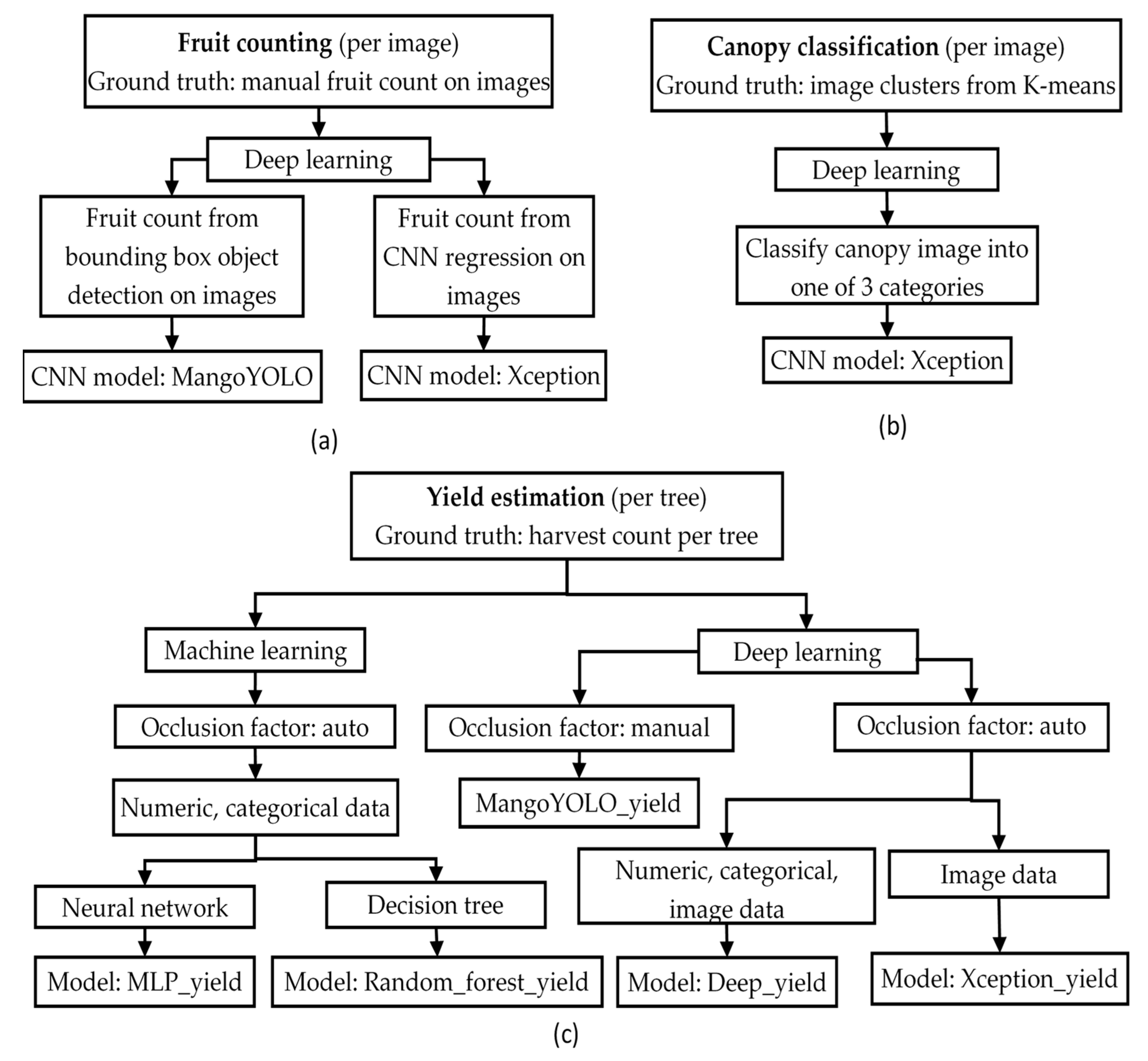
2.3. Fruit Counting and Canopy Classification

2.3.1. Fruit Counting

Two different approaches were trialled for counting visible fruits on tree images. The MangoYOLO model was used to detect fruit within images and add bounding boxes around the fruit, with the number of bounding boxes accepted as the count of visible fruit in an image. As an alternative, the Xception_count model was trained to directly predict fruit numbers in images through CNN regression. CNN regression is quicker and easier to train compared to the object detection method because the regression method does not require bounding box labelling, but rather uses a CNN feature extractor with a final layer of a regression head to provide a fruit load estimate. However, this approach requires accurate ground truth fruit count on a large number of individual trees for use in the training of the CNN regression model. Detail on the two approaches follow:
(i) 
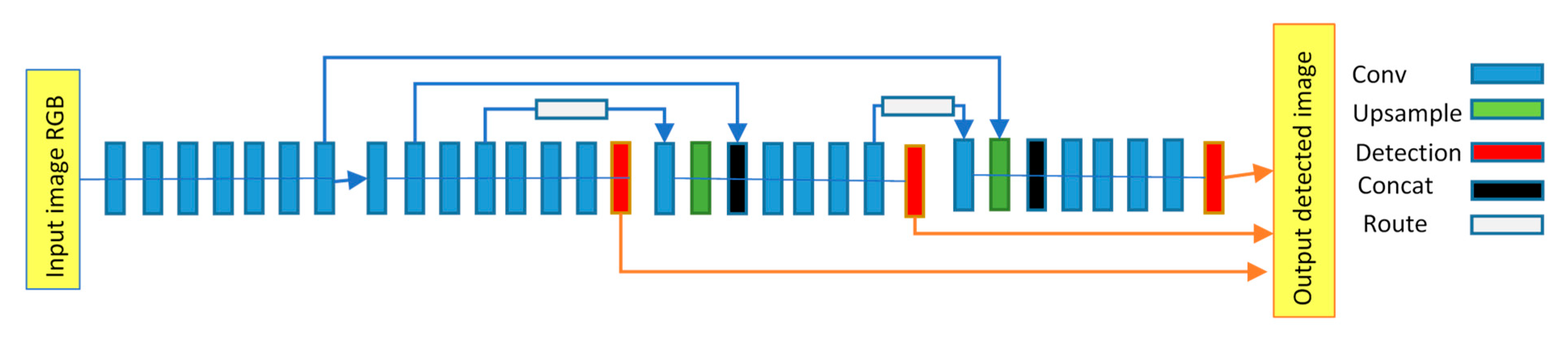
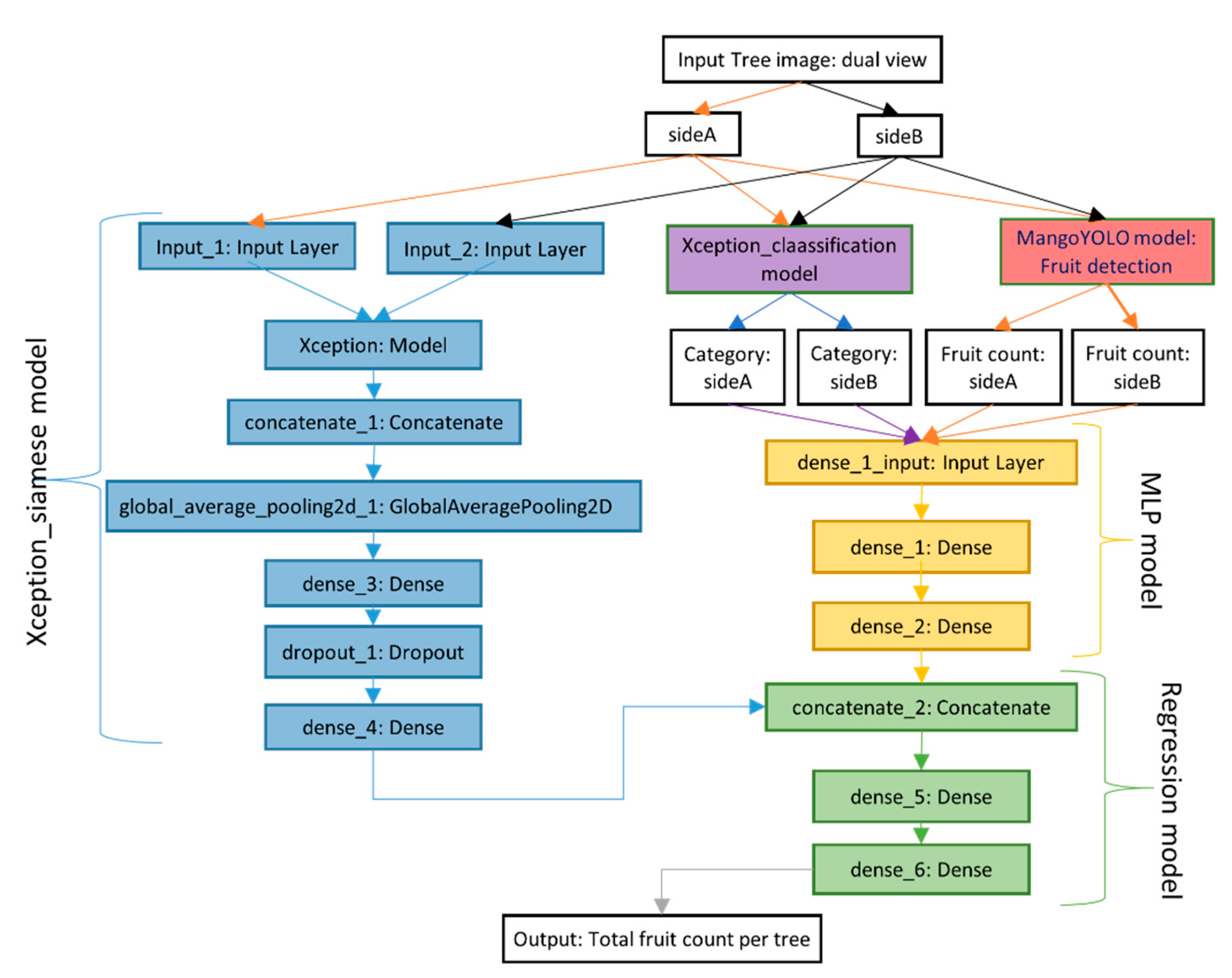
MangoYOLO model: MangoYOLO [3] is a deep learning CNN fruit detection and localization model optimized for speed, computation, and accuracy through re-design of the YOLO object detection framework. MangoYOLO model detects mango fruit, then draws and counts bounding boxes on the detected fruits on tree images. MangoYOLO is comprised of a total of 33 layers, including 3 detection, 2 route, 2 up-sample and 26 convolutional layers (Figure 2). The MangoYOLO model adopted from [3] had been pre-trained on 1300 images containing 11,820 mango fruits and implemented with OpenCV-python v4. The class confidence and NMS thresholds for the MangoYOLO model were set to 0.24 and 0.45, respectively.
(ii) 
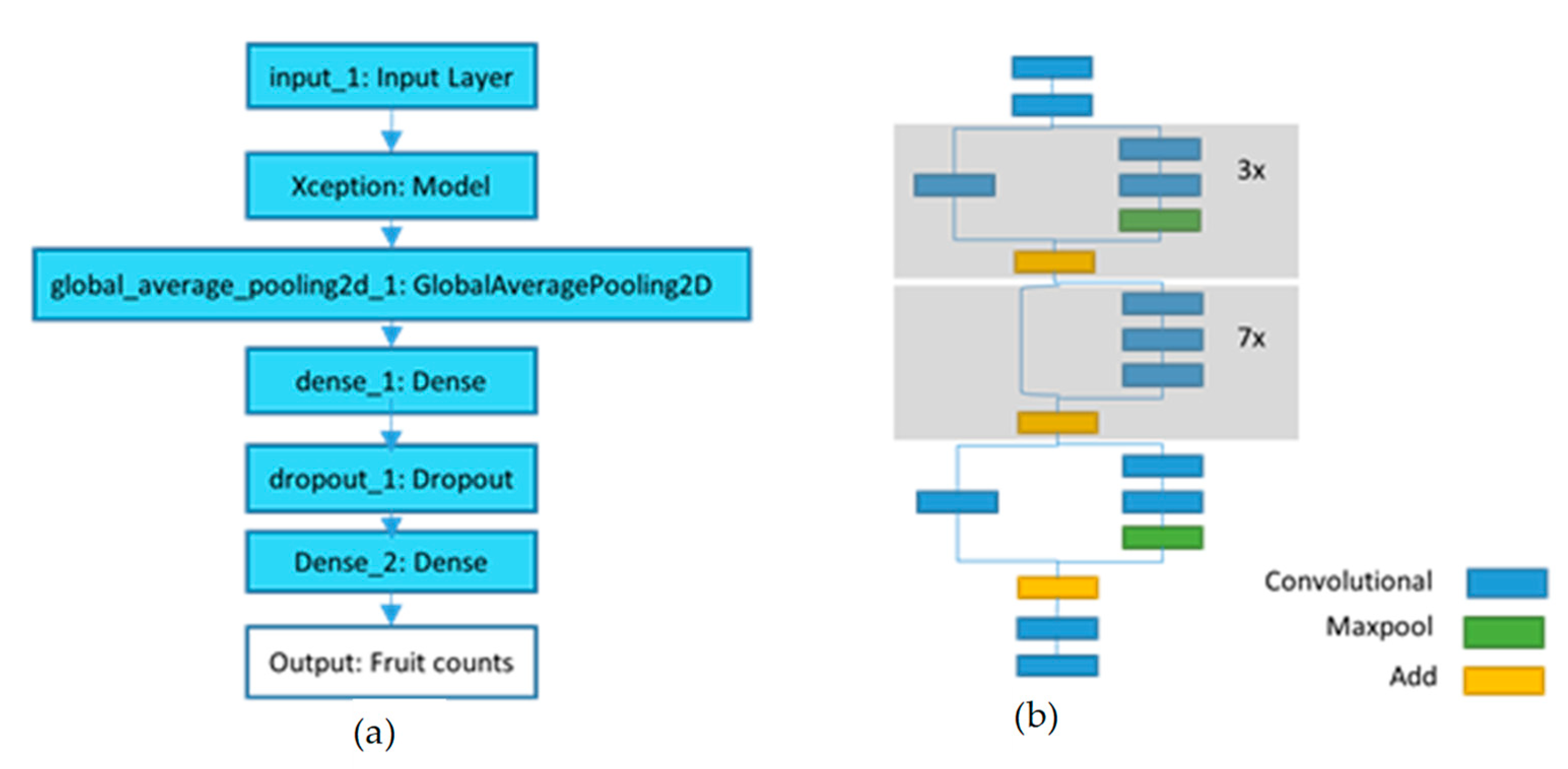
Xception_count model: The Xception _count model was trained to directly predict fruit number on tree images using CNN regression. As number of sample tree images in current training set seemed small for training the regression model, fruit counts from MangoYOLO model on large image set was utilized as ground truth fruit count for training Xception_count model.
“Xception” [14] is a deep learning CNN model with an input resolution of 299 × 299 pixels. The base (without the final classification layers) of the Xception model was imported from the Keras deep learning library and used inside the Xception_count model. The input resolution was changed to accept input images of 1024 × 1024 pixels. A regression head which was comprised of four layers was added to this base model and a global spatial pooling layer (GlobalAveragePooling2D) was used on the output of the base model (Figure 3). The pooling layer was followed by a connected (Dense) layer consisting of 1024 neurons, “relu” activation function and a Dropout (0.65) layer. Dropout [15] helps in preventing neural networks from overfitting by randomly dropping out the fraction of neuron inputs to 0 at each update during training. The final layer is a dense layer with a ‘linear’ activation function.
The Xception_count model was trained on 988 mango tree canopy images of 494 tress (i.e., images of two sides of each tree) from orchard A in 2017. The original images (2448 × 2048 pixels) were resized (1024 × 1024 pixels) as input variables to the model. Fruit counts on each image obtained from the MangoYOLO model [3] were normalized to use as target values for model training. The model was initialized with random weights, i.e., no transfer learning was implemented. Training consisted of 50 epochs, using a batch size of 2 and a learning rate of 1 × 10⁻⁴. The Xception_count model was compiled with the MSE (Mean Squared Error) loss function and “adam” [16] optimizer. MSE is a commonly used loss function for regression modelling and is computed as the mean of the squared difference between estimated and actual values.
The intermediate output from the trained Xception_model was used as an input to the Xception_classification model.

2.3.2. Xception_Classification Model

The aim of the Xception_classification model was to categorize canopies with similar fruit patterns into one of three categories, using both images (dual view) of a given tree. The features learnt by the Xception CNN block of a trained Xception_count model was utilized for training of an Xception_classification model for purpose of canopy categorisation. The Xception_classification model was of the same architecture as the Xception_count model (Figure 3) except for two changes:
  • The Dense_2 layer of Xception_classification model consisted of 3 neurons for 3 canopy categories/classes and “sigmoid” activation function compared to 1 neuron and ‘linear’ activation function for predicting continuous values in Xception_count model.
  • The Xception_classification model was compiled with “categorical_crossentropy” loss function compared to MSE loss function in Xception_count model. Cross-entropy is a commonly used loss function for multi-class classification task. Cross-entropy is based on the maximum likelihood (probability distribution across multiple classes). This function tries to minimize the mean difference between the actual and estimated probability distributions for all classes considered.
The Xception base of Xception_classification model was initialized with the learned weights from the Xception base of Xception_count model. The feature vector from the intermediate layer of the trained Xception_count model was utilized as input, along with reference categories obtained from the k-means clustering algorithm.
To creating ground truth categories for canopy classification, K-means clustering was applied on the output vectors from the ‘global_average_pooling2d_1’ layer of the Xception_count (Figure 3) model (input size 1024 × 1024 pixels) for whole orchard A 2017-season tree images. The K-means algorithm clusters data by separating samples to n groups of equal variances, using n = 3 in this case.
Since there was no ground truth category/label for the images being clustered, the Silhouette coefficient [17] was calculated to assess the effectiveness of the categorisation in terms of creating unique groups. The Silhouette value is a measure of similarity of an object to its own cluster compared to other clusters. Silhouette coefficient is calculated from the measure of mean distance between a sample and (i) all other points in the same cluster, and (ii) all other points in the next nearest cluster. The coefficient varies from −1 to 1, with higher scores for better defined clusters. Default parameters from the sklearn library were used for both k-means clustering and Silhouette metrics calculation. The number of clusters varied from 2 to 5 but three clusters were chosen on all blocks because of a relatively good Silhouette coefficient and a relatively balanced distribution (Table 3).
From qualitative inspection of images of the three groups, images from cluster (c) were generally distinct from those of clusters (a) and (b), having few or no fruit and denser foliage. There were no consistent differences between images of clusters (a) and (b), although trees with open canopies tended to belong to cluster (a) (Figure 4).
For training and tuning, 2017 images of orchard A (all 494 trees) were split randomly, with 90% for training and 10% for tuning. The 2018 image set of the same orchard was used as a test set. Images were used at a resolution of 1024 × 1024 pixels. Training involved 50 epochs with batch size = 2 and learning rate = 1 × 10⁻⁴.
The Xception_classification model was used to classify input tree images into three categories (low, medium and high visible fruit load), for use as input categories into the yield estimation models of the current study.

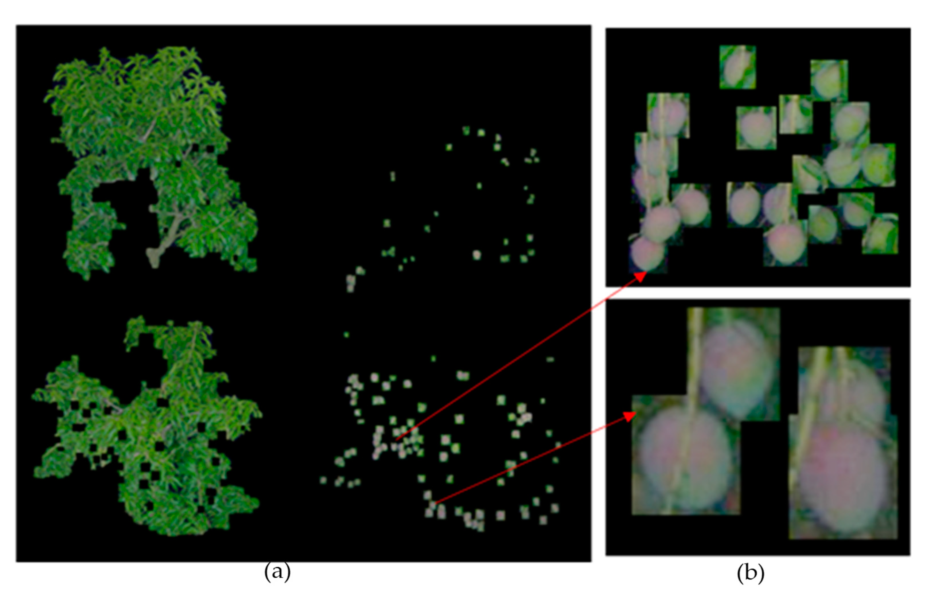
2.4. Canopy and Fruit Region Extraction

2.4.1. Canopy Extraction

After the fruit regions were extracted from the bounding box coordinates returned by the MangoYOLO model, a colour segmentation technique followed by contour fitting was used to extract the foliage of the canopy into a blank image. Images were converted from BGR to HSV range using the OpenCV function. Colour segmentation was done by selecting a range of green colour (HSV range lower = (33, 80, 40) and upper = (102, 255, 255) followed by morphological operations (conversion to grayscale, median blurring, adaptive thresholding (mean) and closing). In the resultant binary image, OpenCV’s contour fitting function was used to obtain the contour of the foliage from the image (Figure 5).

2.4.2. Shape Fitting

The mango fruit shape can be approximated using an ellipse [18,19,20]. The use of ellipse fitting technique has been used to discriminate fully exposed mango fruit from partly occluded fruit in canopy images for fruit size estimation [21,22]. A similar approach was implemented in the current study.
Each input image was processed using MangoYOLO for detection of fruit. Each RoI (fruit region inside bounding box) was individually processed for shape fitting. ROIs were converted to grayscale and sharpened to highlight the fruit edges using OpenCV functions. The resultant image was converted to binary image using the adaptive thresholding (mean) algorithm followed by morphological closing operation. OpenCV’s contour fitting function and ellipse fitting algorithm was used to fit an elliptical shape on the binary image.
Ellipses fitted to partially occluded fruits were more eccentric compared to fully visible (entire) fruit (Figure 5). An eccentricity value of 0.75 was used as a threshold to discriminate partially occluded fruit from non-occluded fruit, as recommended by [20]. The eccentricity threshold is expected to vary for cultivars which differ in fruit shape. The area of ellipses for full and partly occluded fruit were summed for each tree image. Similarly, canopy area in an image was estimated. This output was used as training data for MLP_yield and Random_forest_yield models.
The canopy (foliage and fruit) of ABC-x training set tree images was segmented and images from the two inter-row faces of each tree placed in a new single image. This process resulted in half the number of images in a new dataset. The MangoYOLO model was used to detect fruits on the images, with the coordinates of the detected bounding box used to extract the RoI (fruit regions) into a blank image. Similarly, the canopy extraction contour was used as a mask to segment the foliage into a blank image. Finally, the four images of extracted fruit and canopy regions (2448 × 2048 pixels each) were aligned into a single image (4896 × 4096 pixels) and resized (1024 × 1024 pixels) (Figure 6) for input to the Xception_yield model.

2.5. Yield Estimation

2.5.1. Overview

Four machine learning models were created to directly predict the total fruit number per tree from the input of dual-view images, with benchmarking to a Mango_YOLO estimate of visible fruit per tree corrected using an orchard wide occlusion factor, and to orchard harvest data. Since each yield estimation model was comprised of several small modules (different architecture, different input data types and different input resolutions), the training parameters vary across models. These parameters were tuned to obtain best results while also considering the available computational resources (e.g., GPU memory).
The 2017 images of sample trees ABCx were 80:20 split randomly into a training and a test set for training MLP_yield, Random_forest_yield and Deep_yield models. However, a train:test split of 90:10 was used for the Xception_yield model to increase the amount of training data because this method trains on reconstructed image (two sides of a tree images merged into a single image) which reduced actual train/test set by 50%.
Yield estimates from the five methods were compared to human based count of fruit per tree using linear regression analysis (slope, intercept, RMSE and R2 values).

2.5.2. MLP_Yield Model

The MLP_yield model employed MLP regression in prediction of the total fruit number per tree using the inputs of the count of fruit on the two sides of tree image, number of exposed (fully visible) fruit, number of partially occluded fruit, canopy foliage area (pixel), fully visible fruits total area (pixel), and partially occluded fruit total area (pixel).

Network Architecture

The MLP_yield model consisted of a stack of multiple Fully Connected (FC) layers of neurons (12-6-1 architecture). The input layer (dense layer_1) consisted of 12 neurons to match the number of input variables. The intermediate layer (dense layer_2) consisted of 6 neurons. Both first and second layers used the ‘relu’ activation. The final layer (output_layer) consisted of a single neuron to predict fruit counts using a ‘linear’ activation function.

Training

The MLP_yield network involves 12 input variables (6 for each image side of a tree- cT, cF, cO, RpF, RpO and RpC, Table 4). Fruit count data (cTa, cFa, cOa, cTb, cFb, cOb) and target ground truth harvest count per tree were normalized by dividing by the maximum values found in the training dataset, i.e., 200 for fruit count per tree and 600 for harvest count per tree All three layers of MLP_yield model was initialized using ‘uniform’ weights and trained for 200 epochs with a batch size of 4. The model was compiled with a MSE loss and an Adam optimizer with learning rate of 1 × 10⁻³.

2.5.3. Random_Forest_Yield Model

The Random_forest_yield model was used for estimating total fruit number per tree based on input parameters same as MLP_yield model but utilizing an ensemble of decision trees for regression.

Network Architecture

Random forest [23] is a simple yet accurate machine learning algorithm used for classification and regression tasks [24]. It builds ‘forests’ from an ensemble of decision trees to increase predictive accuracy. Random forest adds randomness while splitting a node by searching for best feature from a random subset of features rather than searching for most important features within the larger set. This procedure helps control over-fitting of the model.

Training Method

RandomForestRegressor from “sklearn” library was used with default values (max_depth = None, n_estimators = 100, criterion = “mse”) for model training on the same training data used by the MLP_yield model.

2.5.4. Deep_Yield Model

Network Architecture

The Deep_yield model was composed of five networks- MangoYOLO, MLP, Regression, Xception_siamese and Xception_classification (Figure 7).
The MLP block: The Multi Layered Perceptron (MLP) consisted of a stack of multiple Fully Connected (FC) layers of neurons (8-4 architecture). The input layer (dense_1) contained 8 neurons (6 for the 2 category vectors each having 3 elements obtained for each side of tree images from Xception_classification model, and 2 neurons for the fruit count on two sides of image obtained from MangoYOLO model). The final layer (dense_2) consisted of 4 neurons to match the number of input nodes (i.e., the output of the Xception_siamese network) in the model. An activation function “relu” was used for both dense layers.
The Siamese block: With a Siamese network it is possible to train a single model with multiple inputs. The Xception_siamese network takes RGB input images (299 × 299 pixels) for each side of a tree as input to the Xception model (Figure 7). The outputs for each image side from Xception model of the Xception_siamese network were concatenated (concatenate_1 layer) and global average spatial pooling operation applied. The data was further processed through Fully Connected (FC)/dense layers- dense_3 and dense_4 having 1024 and 4 neurons, respectively. A dropout layer (dropout_1) with dropout value = 0.65 was used before the final layer to prevent the model from overfitting. All the dense layers used “relu” activation function. The final layer (dense_4) consisted of 4 neurons to match the output nodes of the MLP model.
The Regression block: The regression model consisted of 1 concatenation layer and 2 FC dense layers (Figure 7). The concatenation layer (concatenate_2) concatenated the outputs of Xception_siamese and MLP models. The dense layer (dense_5) with “relu” activation function consisted of 4 neurons to match the number of input nodes. The final layer (dense_6) consisted of 1 neuron and a “linear” activation function to predict continuous data (total fruit counts per tree).

Training

The ABC-x training set was used in development of a Deep_yield model using 200 epochs with learning rate = 1 × 10⁻³, loss function = MSE, optimizer = Adam and batch size = 8. The Xception network inside the Xception_siamese model was initialized with pre-trained ImageNet weights available from the Keras library. For model training, the target values (harvest count) were normalized by dividing with the maximum harvest count value.

2.5.5. Xception_Yield Model

Network Architecture

The architecture of the Xception_yield model was the same as that of the Xception_count model (Figure 3), while the input was altered to the reconstructed image, i.e., canopy and fruit regions of both sides of a tree extracted to a single image.

Training Method

The model was compiled with MSE loss, Adam optimizer and trained for 50 epochs with batch size of 2 and learning rate of 1 × 10⁻⁴. Transfer learning was not used and the weights for the CNN model were initialized at random values.

3. Results and Discussion

3.1. Fruit Counting Using Xception_Count Compared to MangoYOLO

The class activation map of the trained Xception_count model was visualized on the final convolutional layer (block14_sepconv2_act) to illustrate the regions in images utilized by the model for prediction of fruit numbers. The Grad-CAM [25] visualization technique revealed that the model was indeed activated by the fruit regions rather than other objects (Figure 8).
Similarly, the visualization of Xception_yield model showed that the model used the fruit regions in the image for prediction of the total fruit count in the canopy (Figure 9).
The Xception_count and MangoYOLO models were compared in terms of estimates of all trees in orchard A in both 2017 and 2018 (Table 5). The coefficient of determination (R2) for the linear regression of the results of the two methods was high in both years, but the Xception_count underestimated fruit load relative to the MangoYOLO model.
Relative to a manual harvest count reference of the sample trees, the result of the Xception_count model was not as precise (lower R2 on human count) or accurate (slope less < 1, intercept > 0) as the MangoYOLO model result in prediction of fruit load of trees in a different year to that used for training (Table 6).

3.2. Canopy Categorization

The Xception_classification model was trained on all 2017 images of orchard A images for classification to one of three categories, with 80, 99 and 94% correct classifications achieved for categories a, b and c, respectively, relative to the k-means clustering reference values (Table 7).
The Xception_classification model (trained on 2017 orchard A images) was further tested on 2017 orchard C images, achieving 65, 88 and 97% correct classifications achieved for categories a, b and c, respectively (Table 8).
These results are consistent with the qualitative assessment, i.e., that category (c) images were the most distinct, while a greater level of confusion exists between categories (a) and (b).

3.3. Correlates to Occlusion Factor

To predict total fruit load from tree images requires visual indicators within the image that are correlated to the number of fully occluded fruit. It was hypothesised that the number of partly occluded fruit normalised to the number of visible fruit would be correlated to the ratio of fully occluded fruit normalised to the number of visible fruit. However, while the number of partly occluded fruit was tightly correlated (R2 around 0.9) to the number of visible fruit per tree, relations involving harvest count or hidden fruit were poor (Table 9). The exception was a strong correlation (R2 around 0.9) noted between the ratio of hidden to harvest count and the ratio of full exposed to harvest count (Table 9), a relationship of no predictive value in that harvest count is required. With no obvious relationship between visible canopy features and hidden fruit count, this result does not bode well for use of a deep learning model to predict total fruit load of a tree.

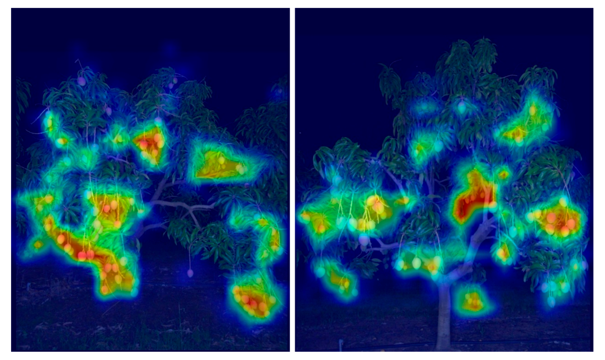
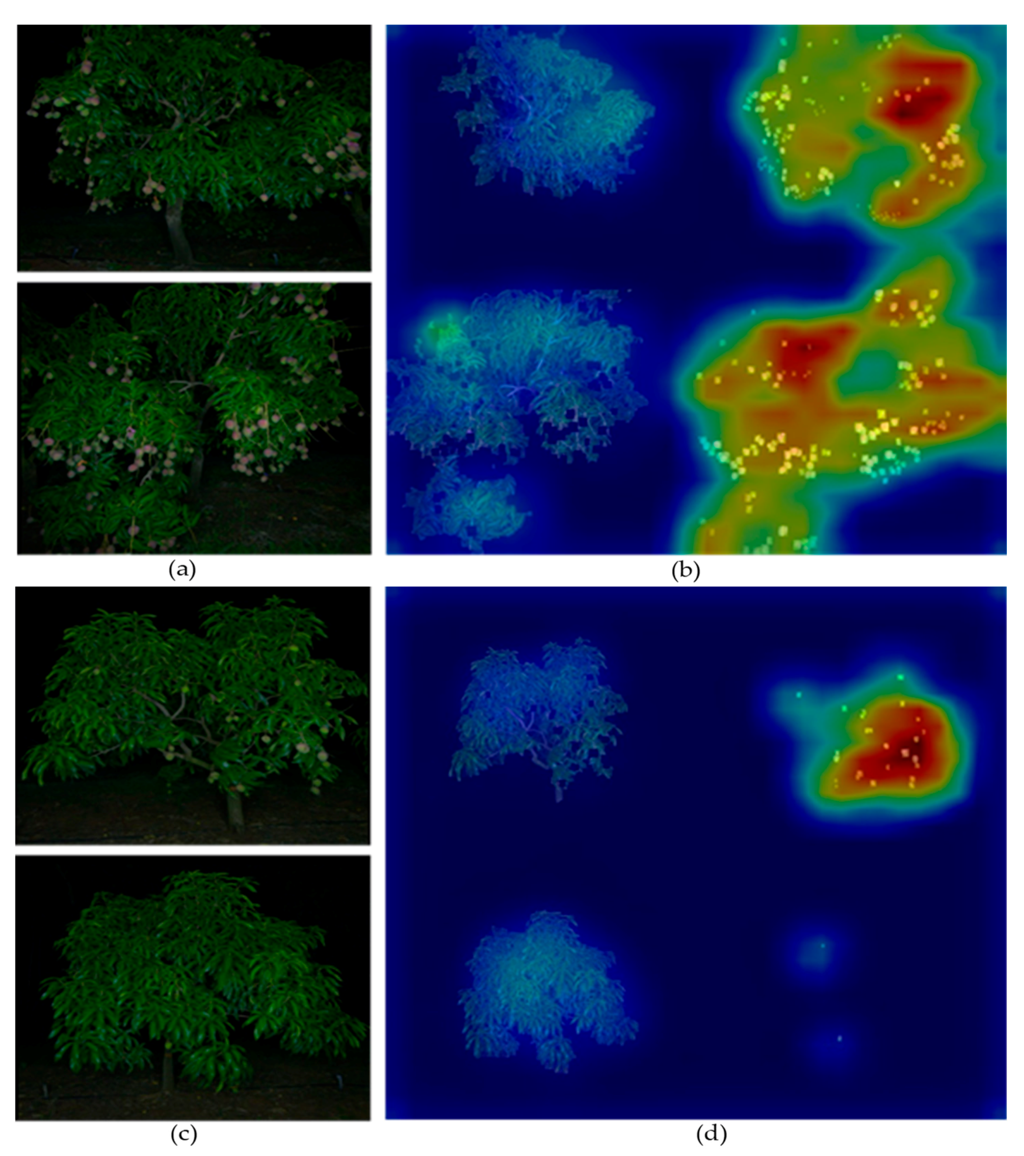
3.4. Feature Importance in Models

While the deep yield models are essentially black boxes, it is useful to gain some insight into the attributes used, the better to train such models and to anticipate prediction failures.
The Random forest regressor used by Random_forest_yield model for prediction of harvest count placed highest weight on fruit count per tree (cTa and cTb), followed by count of fully visible fruit, count of partly occluded fruit and ratio of canopy area to total image area, a surrogate for canopy size (Table 10). The ratio of number of partially occluded fruit area to canopy area was hypothesised to represent a foliage density index, however it was low in weighting.
For the same orchard A used in this study, Stein et al. [6] observed almost no relationship between the canopy volume (estimated as LiDAR voxel count) and yield (fruit count per tree). A poor correlation (R2 = 0.21 and 0.17, respectively) between canopy attributes of canopy volume and trunk circumference and fruit load was also reported for the same orchard [1]. These observations are consistent with the low weighting assigned to the attributes related to canopy size (e.g., RpC).

3.5. Model Performance in Prediction of Tree Fruit Load

The slope of the correlation between MangoYOLO count of two images per tree and harvest count of sample trees was only 0.44 (Table 11) and 0.32 (Table 12) in 2017 and 2018, respectively, indicating that a large proportion of fruits were not visible in dual view imaging. Use of an occlusion factor calculated using the 2017 ABC sample set to adjust the MangoYOLO_yield model result improved the slope of the predicted to harvest count to 0.89 (Table 11) and 0.67 (Table 12), respectively.
The MangoYOLO_yield method was compared to the four methods of direct yield estimation in prediction of the training set (Table 11) and test sets (Table 12), using images of 2017 and 2018 seasons, respectively. The best prediction result for the ABCx-2017 set was achieved with the Random_forest_yield model (R2 = 0.98 and RMSE = 17.8) (Table 11), however for the ABC-2018 set, the MangoYOLO_yield method using an occlusion factor obtained for the same year achieved the best result, followed by the Random_forest_yield method (Table 12). The direct yield estimation models were therefore not robust in prediction of a population of another season.
Relative to packhouse count of the entire 2017 orchards, the results of the direct prediction models were superior to the estimate from the MangoYOLO_yield model (Table 13). The Random_forest_yield model provided the best estimate for both orchard A and the combined ABC orchards, with a 2.5 and 2.3% error, respectively, with the Deep_yield model providing the best result for orchards B and C, with a 0.1 and −3.5% error, respectively (Table 13). The low prediction error of the 2017 sample test set and the 2017 orchard total indicates a robustness issue for the model, with good performance only in the year that the training samples were collected.

4. Conclusions

The current work was inspired by reports of direct estimation of total fruit load per tree from tree images [10,11,12]. The use of machine learning models trained directly on fruit number per tree rather than fruit number per image avoids the need for manual estimation of an occlusion factor every season. This approach also avoids the need for bounding box annotation of training images. However, initial workload is increased in this method in that many trees must be human counted for training of the models.
To achieve direct prediction of tree fruit load from tree images this there must be clues within the images as to the proportion of hidden fruit, such as the ratio of partly occluded fruit to total visible fruit in an image. The direct input of such indices should improve model effectiveness and reduce training effort. However, no such attribute correlates were identified.
In this study the shallow ANNs implementation in previous attempts [10,11,12] for direct estimation of tree crop load were replaced with deep learning convolutional neural networks (CNNs). Random forest and multi-layered perceptron (MLP) models were also trialled for estimation of a correction factor per tree. The supervised machine learning methods for direct estimation of fruit load per tree delivered an improved prediction outcome over the result achieved using a machine vison count corrected by occlusion factor for data of the season/orchard from which training data was acquired, but the performance of these models on a new season data (test set images) was poorer than the reference method. This result indicates that training on one season of data was insufficient for the development of a robust model. This outcome can be attributed to variability in tree architecture and foliage density between seasons and between orchards, such that the characters of the canopy visible from the interrow that relate to the proportion of hidden fruit are not consistent. Therefore, training of the yield estimation models across several seasons and orchards is recommended. While a robust method for estimate of total fruit load per tree from canopy images has not been demonstrated, several methods have been presented that should serve to extend the ‘toolkit’ used in machine learning based yield estimation methods.

Author Contributions

Conceptualization, A.K. and K.B.W.; image acquisition, A.K. and Z.W., methodology, A.K.; software, A.K.; validation, A.K. and K.B.W.; formal analysis, A.K. and K.B.W.; investigation, A.K.; data curation, A.K.; writing—original draft preparation, A.K.; writing—review and editing, K.B.W.; visualization, A.K.; supervision, K.B.W. and Z.W.; project administration, K.B.W.; funding acquisition, K.B.W. All authors have read and agreed to the published version of the manuscript.

Funding

This work received funding support through Horticulture Innovation Australia from the Australian Government Department of Agriculture and Water Resources as part of its Rural R&D Profit program (project ST19009, Multiscale monitoring tools for managing Australian tree crops).

Data Availability Statement

The data (images and annotations) used for training/testing MangoYOLO fruit detection model is available at figshare.com (https://figshare.com/articles/dataset/MangoYOLO_data_set/13450661/2 (accessed on 10 February 2021)). The data (images and fruit counts) analysed in this study are available at figshare.com (https://figshare.com/articles/dataset/Mango_deep_yield_dataset_koirala_et_al_2021/14033993 (accessed on 10 February 2021)).

Acknowledgments

A.K. acknowledges receipt of an Australian Regional Universities Network scholarship, and Z.W. was funded by a CQU Early Career Fellowship. Farm support from Groves farm and Simpsons farm is appreciated. Image acquisition support from Nicholas Anderson is appreciated. A modified form of this manuscript comprised a chapter in the PhD thesis of A.K. The feedback of anonymous thesis reviewers is appreciated.

Conflicts of Interest

The authors declare no conflict of interest.

References

  1. Anderson, N.; Underwood, J.; Rahman, M.; Robson, A.; Walsh, K. Estimation of fruit load in mango orchards: Tree sampling considerations and use of machine vision and satellite imagery. Precis. Agric. 2018. [Google Scholar] [CrossRef]
  2. Koirala, A.; Walsh, K.B.; Wang, Z.; McCarthy, C. Deep learning—Method overview and review of use for fruit detection and yield estimation. Comput. Electron. Agric. 2019, 162, 219–234. [Google Scholar] [CrossRef]
  3. Koirala, A.; Wang, Z.; Walsh, K.; McCarthy, C. Deep learning for real-time fruit detection and orchard fruit load estimation: Benchmarking of ‘mangoyolo’. Precis. Agric. 2019, 20, 1107–1135. [Google Scholar] [CrossRef]
  4. Payne, A.B.; Walsh, K.B.; Subedi, P.; Jarvis, D. Estimation of mango crop yield using image analysis–segmentation method. Comput. Electron. Agric. 2013, 91, 57–64. [Google Scholar] [CrossRef]
  5. Wang, Q.; Nuske, S.; Bergerman, M.; Singh, S. Automated crop yield estimation for apple orchards. In Experimental Robotics; Springer: Berlin/Heidelberg, Germany, 2013; pp. 745–758. [Google Scholar]
  6. Stein, M.; Bargoti, S.; Underwood, J. Image based mango fruit detection, localisation and yield estimation using multiple view geometry. Sensors 2016, 16, 1915. [Google Scholar] [CrossRef] [PubMed]
  7. Moonrinta, J.; Chaivivatrakul, S.; Dailey, M.N.; Ekpanyapong, M. Fruit detection, tracking, and 3D reconstruction for crop mapping and yield estimation. In Proceedings of the 11th International Conference on Control Automation Robotics & Vision (ICARCV), Singapore, 7–10 December 2010; IEEE: New York, NY, USA, 2010; pp. 1181–1186. [Google Scholar]
  8. Liu, X.; Chen, S.W.; Aditya, S.; Sivakumar, N.; Dcunha, S.; Qu, C.; Taylor, C.J.; Das, J.; Kumar, V. Robust Fruit Counting: Combining Deep Learning, Tracking, and Structure from Motion. arXiv 2018, arXiv:1804.00307. [Google Scholar]
  9. Sarron, J.; Malézieux, E.; Sane, C.A.B.; Faye, E. Mango yield mapping at the orchard scale based on tree structure and land cover assessed by UAV. Remote Sens. 2018, 10, 1900. [Google Scholar] [CrossRef] [Green Version]
  10. Črtomir, R.; Urška, C.; Stanislav, T.; Denis, S.; Karmen, P.; Pavlovič, M.; Marjan, V. Application of Neural Networks and Image Visualization for Early Forecast of Apple Yield. Erwerbs-Obstbau 2012, 54, 69–76. [Google Scholar]
  11. Cheng, H.; Damerow, L.; Sun, Y.; Blanke, M. Early yield prediction using image analysis of apple fruit and tree canopy features with neural networks. J. Imaging 2017, 3, 6. [Google Scholar] [CrossRef]
  12. Qian, J.; Xing, B.; Wu, X.; Chen, M.; Wang, Y.a. A smartphone-based apple yield estimation application using imaging features and the ANN method in mature period. Sci. Agric. 2018, 75, 273–280. [Google Scholar] [CrossRef]
  13. Chen, S.W.; Shivakumar, S.S.; Dcunha, S.; Das, J.; Okon, E.; Qu, C.; Taylor, C.J.; Kumar, V. Counting apples and oranges with deep learning: A data-driven approach. IEEE Robot. Autom. Lett. 2017, 2, 781–788. [Google Scholar] [CrossRef]
  14. Chollet, F. Xception: Deep Learning with Depthwise Separable Convolutions. In Proceedings of the IEEE Conference on Computer Vision and Pattern Recognition, Honolulu, HI, USA, 21–26 July 2017; IEEE: New York, NY, USA, 2017; pp. 1251–1258. [Google Scholar]
  15. Srivastava, N.; Hinton, G.; Krizhevsky, A.; Sutskever, I.; Salakhutdinov, R. Dropout: A Simple Way to Prevent Neural Networks from Overfitting. J. Mach. Learn. Res. 2014, 15, 1929–1958. [Google Scholar]
  16. Kingma, D.P.; Ba, J. Adam: A Method for Stochastic Optimization. arXiv 2014, arXiv:1412.6980. [Google Scholar]
  17. Rousseeuw, P.J. Silhouettes: A graphical aid to the interpretation and validation of cluster analysis. J. Comput. Appl. Math. 1987, 20, 53–65. [Google Scholar] [CrossRef] [Green Version]
  18. Charoenpong, T.; Chamnongthai, K.; Kamhom, P.; Krairiksh, M. Volume measurement of mango by using 2D ellipse model. In Proceedings of the International Conference on Industrial Technology, IEEE ICIT’04, Hammamet, Tunisia, 8–10 December 2004; IEE Corpoarate office: New York, NY, USA, 2004; pp. 1438–1441. [Google Scholar]
  19. Kader, A.A. Fruit maturity, ripening, and quality relationships. In Proceedings of the International Symposium Effect of Pre-& Postharvest factors in Fruit Storage, Warsaw, Poland, 3 August 1997; Acta Hortic. 485. IEE Corpoarate office: New York, NY, USA, 1997; pp. 203–208. [Google Scholar] [CrossRef]
  20. Nanaa, K.; Rizon, M.; Rahman, M.N.A.; Ibrahim, Y.; Aziz, A.Z.A. Detecting mango fruits by using randomized hough transform and backpropagation neural network. In Proceedings of the International Conference on Information Visualisation, Paris, France, 16–18 July 2014; IEEE: New York, NY, USA, 2014; pp. 388–391. [Google Scholar]
  21. Wang, Z.; Walsh, K.B.; Verma, B. On-Tree Mango Fruit Size Estimation Using RGB-D Images. Sensors 2017, 17, 2738. [Google Scholar] [CrossRef] [PubMed] [Green Version]
  22. Wang, Z.; Koirala, A.; Walsh, K.; Anderson, N.; Verma, B. In Field Fruit Sizing Using A Smart Phone Application. Sensors 2018, 18, 3331. [Google Scholar] [CrossRef] [PubMed] [Green Version]
  23. Breiman, L. Random forests. Mach. Learn. 2001, 45, 5–32. [Google Scholar] [CrossRef] [Green Version]
  24. Liaw, A.; Wiener, M. Classification and regression by randomForest. R News 2002, 2, 18–22. [Google Scholar]
  25. Selvaraju, R.R.; Cogswell, M.; Das, A.; Vedantam, R.; Parikh, D.; Batra, D. Grad-CAM: Visual Explanations from Deep Networks via Gradient-Based Localization. In Proceedings of the IEEE International Conference on Computer Vision (ICCV), Venice, Italy, 22–29 October 2017; pp. 618–626. [Google Scholar]
Figure 1. Flowchart of methods used―for count of fruit in each image (a), for canopy classification (b) and for yield estimation (c).
Agronomy 11 00347 g001
Figure 2. Block diagram of MangoYOLO model.
Agronomy 11 00347 g002
Figure 3. Xception_count model (a and schematic of Xception base model (without top classification layers) (b).
Agronomy 11 00347 g003
Figure 4. Example images from the three categories based on Silhouette score. Typical image in cluster-a (a), cluster-b (b) and cluster-c (c).
Agronomy 11 00347 g004
Figure 5. Ellipse fitting and canopy extraction. (a) Fruit enclosed by blue ellipse contour and red ellipse contour represent the fully exposed fruit and partly occluded fruit, respectively. (b) Area enclosed by the white contour around the tree represents the segmented canopy foliage area. Eccentricity values are displayed.
Agronomy 11 00347 g005
Figure 6. (a)—a single image reconstructed from images of two sides of a canopy, with fruits and canopy separated. (b)—closeup view of fruit images.
Agronomy 11 00347 g006
Figure 7. Block diagram of the Deep_yield model.
Agronomy 11 00347 g007
Figure 8. Grad-CAM visualization of activation map of the final convolution layer of Xception_count model trained to directly predict fruit count on input images. Example given are images from two sides of one tree.
Agronomy 11 00347 g008
Figure 9. Grad-CAM visualization of the activation heatmap of the final convolutional layer of Xception_yield model on the reconstructed input images. Panels (a,c) present the raw images of two sides of a tree while (b,d) present activation heat-maps of canopy and fruit regions of reconstructed images, respectively. (a): Typical result for tree with fruit on both sides of the canopy. (b): Typical result for tree with fruit on one side of canopy.
Agronomy 11 00347 g009
Table 1. Methods used in (A) counting of fruit in images, (B) classification of canopy images and (C) fruit load (count) of whole tree.
MethodDescription
A. Methods for count of fruit in image
MangoYOLOAutomated fruit detection and counting on tree images based on bounding-box training; a modification of YOLOv3 architecture.
Xception_CountAutomated fruit number estimation on tree images based on CNN regression.
B. Method for classification of canopy
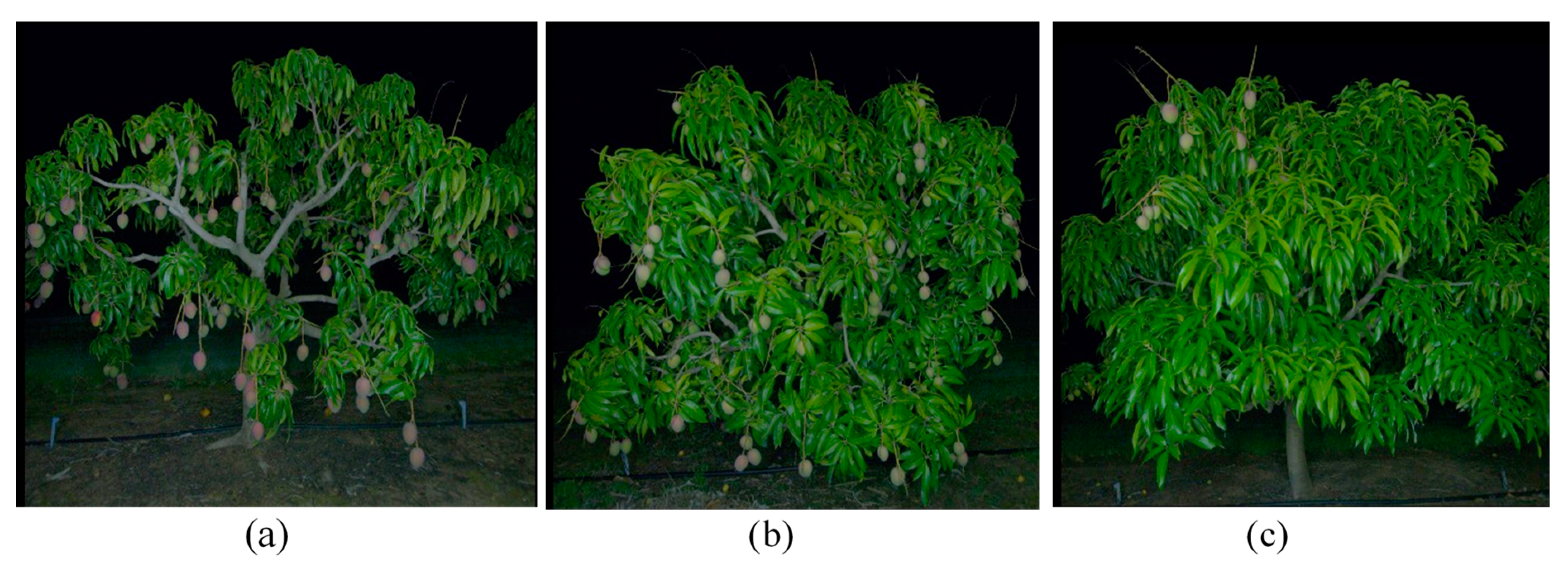
Xception_ClassificationAutomated classification of tree images into 3 categories (low, medium and high visible fruit density) based on image feature learned by Xception_count model.
C. Method for estimation of tree fruit load
Mango_YOLO_YieldEstimate of tree fruit yield based on Mango_YOLO count adjusted using an occlusion factor estimated from manual counts of fruit load of a sample of trees.
MLP_YieldAutomated yield estimation using a MLP neural network with input parameters obtained from canopy and fruit region extraction, including MangoYOLO based estimates of both fully visible and partly occluded fruit number. Partial occlusion of fruit was determined through ellipse fitting.
Random_Forest_YieldAutomated yield estimation using an ensemble of decision trees for regression based on input variables as used in the MLP_yield model.
Deep_YieldAutomated yield estimation based on fruit counts from MangoYOLO model and canopy classification of tree images, using a combination of MLP, Regression, Xception_siamese and Xception_classification blocks.
Xception_YieldAutomated yield estimation based the Xception_count model but extracting canopy and fruit regions of two sides of a tree into a single image as input to the model. This method does not use MangoYOLO.
Table 2. Statistics on the harvest count of sample trees (fruit per tree) for each of two seasons. ABC represent the collection of sample trees from orchards A, B and C.
20172018
OrchardNumber of Sample TreeMeanSDMeanSD
A172078612899
B6279148205134
C1214875274126
ABC35199103191130
A-x 4418776--
B-x 19253160--
C-x 3517190--
ABC-x 98194105--
Table 3. Categorization of tree canopy images from each block into three clusters.
OrchardSilhouette ScoreNumber of Trees in Cluster aNumber of Trees in Cluster bNumber of Trees in Cluster c
2017-A0.4311443344211
2017-B0.46226210476
2017-C0.4982175242113
Total 681690400
Table 4. Description of input variables used for MLP_yield and Random_forest_yield models. Subscripts a and b represent data for side A and side B images of a tree, respectively.
AttributesDescription
cTa, cTbcount of all visible fruit on image from MangoYOLO model (= cF + cO)
cFa, cFbcount of exposed (fully visible) fruit
cOa, cObcount of partially occluded fruit
RpFa, RpFbratio of total pixel area of exposed fruit to the canopy pixel area
RpOa, RpObratio of total pixel area of partially occluded fruit to the canopy pixel area
RpCa, RpCbratio of canopy pixel area to the total image pixel area
Table 5. Linear regression statistics for fruit count using the Xception_count model against the MangoYOLO model for tree images for orchard A (988 images of 494 trees) for 2 seasons. Units for intercept and RMSE are # fruit/image.
YearSlopeInterceptR2RMSE
20170.73112.320.969.12
20180.72819.810.9411.8
Table 6. Linear regression statistics for fruit count of 2018 tree images of orchard A (17 trees, 34 images) by Xception_count and MangoYOLO models developed using 2017 data, against human count of fruit on images. Units for intercept and RMSE are # fruit/image.
ModelSlopeInterceptR2RMSE
Xception_count 0.71513.690.9310.1
MangoYOLO 0.9150.080.985.3
Table 7. Classification relative to ground truth categories from k-means clustering (values in brackets) for the Xception_classification model. Results are of the training set, i.e., the 2017 orchard A image set (988 images of 494 trees).
Xception_Classification (Number of Tree Images)
K Means Classification (Number of Tree Images)Cat aCat bCat c
Cat a (443)387515
Cat b (334)23320
Cat c (211)130198
Table 8. Classification relative to ground truth categories from k-means clustering (values in brackets) for the Xception_classification model. Results are of a test set, i.e., 2017 orchard C (530 images of 265 trees) using a model trained on orchard A images (988 images of 494 trees).
Xception_Classification (Number of Tree Images)
K Means Classification (Number of Tree Images)Cat aCat bCat c
Cat a (175)1141843
Cat b (113)14990
Cat c (242)80234
Table 9. Statistics for linear correlations between combinations of attributes related to the number of partly occluded fruit, non-occluded and hidden (fully occluded) fruit per tree, for image sets ABCx-2017 and ABC2018: (A) count of partly occluded fruit regressed on harvest count of fruit; (B) count of partly occluded fruit regressed on number of visible fruit; (C) ratio of count of hidden fruit to harvest count regressed on ratio of count of fully exposed fruit to harvest count; (D) count of hidden fruit regressed on count of fully exposed fruit; and (E) ratio of count of partly occluded fruit to count of visible fruit regressed on ratio of count of hidden to count visible fruit. For a given tree, harvest count is equivalent to the sum of hidden (fully occluded), partly occluded and fully exposed (non-occluded) fruit, while visible fruit is the total MangoYOLO count for a tree, equivalent to the sum of partly occluded and fully exposed fruit.
Image SetR2SlopeInterceptRatio
A. Partly occluded vs. harvest count
ABCx20170.690.175.410.21
ABC-20180.640.096.710.38
B. Partly occluded vs. visible fruit
ABCx20170.932.527.850.37
ABC-20180.890.280.610.30
C. Ratio of hidden to harvest vs. ratio of fully exposed to harvest
ABCx-20170.89−1.330.91
ABC-20180.91−0.710.71
D. Hidden fruit vs. fully exposed fruit
ABCx-20170.190.8035.8
ABC-20180.251.3537.3
E. Ratio of partly occluded to visible vs. ratio of hidden to visible
ABCx-20170.0070.00750.36
ABC-20180.044−0.0150.33
Table 10. Feature_importance values returned by the Random Forest regressor on the different input variables. Values sum to 1. Refer to Table 4 for the description of variables. The variable with highest weighting (total fruit count) is shown in bold.
cTacFacOaRpFaRpOaRpCacTbcFbcObRpFbRpObRpCb
0.260.070.080.010.010.070.240.060.100.010.010.07
Table 11. Regression statistics for prediction of fruit load per tree, relative to human count. The result for the raw MangoYOLO prediction is included for comparison. Training set prediction results for ABC-x 2017 season sample trees using five methods, all trained with the ABCx 2017 training image set. The data set used for estimation of occlusion factor in MangoYOLO_yield method is shown in brackets. Unit for slope, bias and RMSE is #fruit/tree.
ModelSlopeInterceptR2RMSE
MangoYOLO0.4417.70.69113.4
MangoYOLO_yield (ABCx 2017)0.8936.40.6965.4
MLP_yield0.8136.60.7947.7
Random_forest_yield0.9019.00.9817.8
Deep_yield0.9410.30.9230.4
Xception_yield0.7128.80.9444.8
Table 12. Regression statistics for prediction of fruit load per tree, relative to human count. The result for the raw MangoYOLO prediction is included for comparison. Test set prediction results for ABC 2018 season sample trees using five methods, trained with ABC-x 2017 images. The data set used for estimation of occlusion factor in MangoYOLO_yield method is shown in brackets. Unit for slope, bias and RMSE is #fruit/tree.
ModelSlopeInterceptR2RMSE
MangoYOLO0.3217.30.73143.7
MangoYOLO_yield (ABCx 2017)0.6735.50.7372.7
MangoYOLO_yield (ABC 2017) 0.6333.50.7377.6
MangoYOLO_yield (ABC 2018)0.8344.50.7369.0
MLP_yield0.5030.30.66102.9
Random_forest_yield0.4652.90.6097.4
Deep_yield0.2961.20.34129.1
Xception_yield0.4229.00.72106.3
Table 13. Yield estimation results for prediction of fruit load per orchard block, relative to packhouse count. (A) Packhouse count for fruit number of whole orchards, A, B and C, for season 2017. (B) Prediction results for fruit number of whole orchards, A, B and C, for season 2017 from models trained on orchard ABC-x 2017 data. Value in brackets is the percentage error. Best result (closest to packhouse) is shown in bold.
ABCABC
A. Packhouse count
97,38226,27340,837164,492
B. Model prediction
MangoYOLO_yield (ABCx 2017)58,074 (2.6)16,189 (17.1)17,329 (6.1)91,592 (13.6)
MLP_yield93,879 (−3.6)32,148 (22.4)41,025 (0.5)167,052 (1.6)
Random_forest_yield99,779 (2.5)29,307 (11.5)39,188 (−4.0)168,274 (2.3)
Deep_yield91760 (−5.8)26,307 (0.1)39,399 (−3.5)157,466 (−4.3)
Xception_yield83638 (−14.1)26,022 (−1.0)36,624 (−10.3)146,284 (−11.1)
Publisher’s Note: MDPI stays neutral with regard to jurisdictional claims in published maps and institutional affiliations.

