
Technologies for Forecasting Tree Fruit Load and Harvest Timing—From Ground, Sky and Time


1
Institute for Future Farming Systems, Central Queensland University, Rockhampton 4701, Australia
2
Geco Enterprises Ltd., San Vicente de Tagua, Tagua 2970000, Chile
*
Author to whom correspondence should be addressed.
Agronomy 2021, 11(7), 1409; https://0-doi-org.brum.beds.ac.uk/10.3390/agronomy11071409
Submission received: 27 May 2021
/
Revised: 7 July 2021
/
Accepted: 8 July 2021
/
Published: 14 July 2021
(This article belongs to the Special Issue In-Field Estimation of Fruit Quality and Quantity)
Abstract
:The management and marketing of fruit requires data on expected numbers, size, quality and timing. Current practice estimates orchard fruit load based on the qualitative assessment of fruit number per tree and historical orchard yield, or manually counting a subsample of trees. This review considers technological aids assisting these estimates, in terms of: (i) improving sampling strategies by the number of units to be counted and their selection; (ii) machine vision for the direct measurement of fruit number and size on the canopy; (iii) aerial or satellite imagery for the acquisition of information on tree structural parameters and spectral indices, with the indirect assessment of fruit load; (iv) models extrapolating historical yield data with knowledge of tree management and climate parameters, and (v) technologies relevant to the estimation of harvest timing such as heat units and the proximal sensing of fruit maturity attributes. Machine vision is currently dominating research outputs on fruit load estimation, while the improvement of sampling strategies has potential for a widespread impact. Techniques based on tree parameters and modeling offer scalability, but tree crops are complicated (perennialism). The use of machine vision for flowering estimates, fruit sizing, external quality evaluation is also considered. The potential synergies between technologies are highlighted.
Keywords:
yield; estimation; machine vision; remote sensing; correlative; models; fruit; tree; review1. Introduction
1.1. The Need for Fruit Load Forecast
This review considers advances in methods for the yield forecast of tree fruit. Such forecasts can be made at a tree, orchard, whole farm or regional level, depending on the management task. At a farm level, forecasts can inform grower decisions around in-season agronomic practices such as thinning, postharvest requirements such as harvest labor, transportation, storage, and requirements for consumables such as trays and inserts. Improved monitoring also offers great potential for the accumulation of reliable data across time. An experienced agronomist will be able to utilize such a resource, combining this information with knowledge of fruit and tree physiology to provide current season advice and to advise on management practices to optimize orchard development.
Forecasts are also critical to the value chain to inform marketing strategy and practice. For example, a typical advertising campaign is planned over four weeks ahead of harvest. In general, the longer or more involved the value chain, the more demand for accurate forecasts.
A general target for yield forecast is for an estimate within ±5% to 10% of the actual yield, with greater accuracy required for industries tied to processing industries or to other markets of set size, e.g., export markets. For example, winemakers desire errors of no more than 2–3% on forecast production, while a tree fruit producer supplying multiple and easily accessed domestic markets might accept a 10–20% forecast error, depending on production volumes, or operate without a forecast.
Yield forecast has multiple components, including the at-harvest fruit number, size and quality, and harvest timing. Fruit number is the primary determinant of yield, while fruit size and quality are key attributes in terms of consumer acceptability, and therefore, achievable pricing. In-field measurements allow for the forward estimation of the proportions of fruit class distributions on these attributes at harvest, and thus for market planning. The timing of fruit maturation is determined by the timing of flowering and subsequent growth conditions. The combination of harvest timing and fruit load information can be used to estimate a weekly harvest schedule. Advances in techniques for the forecasting of each of these components of yield are presented in the current review.
1.2. Literature Base
In this document, the term ‘orchard’ is used to refer to a management block of fruit trees, i.e., of a common genotype, planting date, irrigation scheduling, management history, harvest unit, etc. A ‘typical’ orchard size is around 1000 plants in 2 ha, but this is dependent on commodity and management practice.
A recent review of the use of machine learning for crop yield prediction reported 567 relevant studies; however, this work primarily refers to annual crops [1]. For the narrower topic of tree fruit yield forecast, the scientific publication rate has risen steeply from a low base in the last decade [2] (Figure 1).
Publications on tree fruit yield estimation have focused on the major crops of apple and citrus, and the tropical crop, mango (68% of records), with researchers primarily located in China, the USA and Australia (Table 1). The majority of work has addressed the use of machine vision using RGB cameras (65% of records), but attention has also been given to the correlation of fruit load to tree structural parameters, as measured proximally (in field) or remotely (by an Unmanned Aerial Vehicle, UAV, or satellite), and to the use of time series and climate data. Work on the use of stereology to streamline manual sampling methods was dominated by the work of Wulfsohn and co-workers. However, to our knowledge, the only reviews on tree fruit crop load estimation published in the last decade have been on the use of deep learning for tree fruit detection using machine vision [3] rather than fruit load estimation per se.
With respect to the topic of the prediction of the time of harvest maturity, a Scopus keyword search (doa 9/4/2021) using the keywords of ‘prediction AND fruit AND harvest AND maturity AND timing’ yields 196 results over the ten-year period (2011–2020). Of these reports, the majority refer to studies using a heat unit methodology, with a few papers referring to the development of heat unit models, or to the use of other indices for the estimation of harvest maturation.
1.3. Types of Models
An empirical model (also referred to as a descriptive model) achieves a forecast through a correlation between measurable variables and the attribute of interest, without regard to the mechanism of the relationship. Empirical models describe the data for the conditions under which the data were collected, but may ‘break’ when used in predictions of future populations, especially when seasonal conditions differ significantly to those for the populations used in development of the model. A mechanistic model (also known as an explanatory model) is based on physical, chemical, or biological laws describing the behavior of constituting parts. Mechanistic models are useful in developing an understanding of a system, but predictive power is limited by the understanding of the system and the complexity of the model.
In a 1998 review of forward estimation of biomass production and yield of horticultural crops, Marcelis et al. [4] noted that attempts to produce mechanistic models of production were generally based on modeling photosynthetic capacity through inputs of leaf area development, light interception, photosynthesis and respiration. In subsequent decades, further attempts have been made to develop mechanistic models of tree fruit production, with notable progress made, e.g., in the QualiTree model for peach trees [5]. These models typically predict fruit growth through the consideration of the tree as a set of subunits competing for resources such as light, photo-assimilates and water. The QualiTree model is probably the most advanced tree fruit mechanistic model, although attempts for other tree crops are advancing, e.g., for mango [6,7].
However, the influence of previous growing cycles increases the complexity of tree fruit systems, as seen in irregular bearing between seasons [8]. This complexity hampers the development of a mechanistic model to estimate production and has prevented the practical use of such models for the forecast of fruit load [9]. This review does not further consider the use of fully mechanistic models in tree fruit forecast, but rather focuses on the use of empirical models based on direct count, either manual or machine vision, or on correlation to environmental conditions or canopy attributes.
Tree fruit producers currently commonly rely on empirical models for the prediction of harvest dates [4]. These models rely on the estimation of thermal time since flowering or a measure of a fruit attribute that is related to maturity.
2. Measurement of Fruit Number
2.1. Benchmarking
2.1.1. Reference Estimates
Any analytical procedure involving the comparison of one method to a ‘reference’ method should include an assessment of the error in the reference method. Methods for fruit load estimation need to benchmark to a reference measurement. Where method validation involves a small number of sample trees in the orchard, the reference value is typically a human count of fruit on-tree, or a human count of fruit harvested from the tree. Such estimates are not error free.
To benchmark a fruit load prediction at a whole orchard level, the reference estimate is commonly estimated from the fruit packout report. However, Paliwal and Jain [10] cautioned that self-reported crop data were not accurate enough for predictive model training for a small holder grain production system, even when the use of the data was explained to the contributors. Similar issues hold for the tree fruit production system. Packhouse record keeping is often lacking, particularly if fruit from several producers or multiple orchards per farm are processed in the same shift, or if orchards are harvested over several dates. Further, harvesting operations may move across several orchards at a time, such that tree crop packout data may not be organized to easily provide orchard level data. The increasing adoption of field bin identification systems and farm data management systems is improving this situation.
Packout fruit numbers can be estimated from records of the number of trays of a given fruit number per tray. While rejected fruit are not packed, a weight is generally taken. The fruit number can then be estimated using an average fruit weight, although the use of the average weight of packed fruit will typically result in an underestimation of the rejected fruit number, as a low fruit weight is a criterion for rejection.
The packout count can be expected to be less than the orchard fruit load as fruit drop may occur between the time of load estimation and harvest as a result of extreme climatic events, disease or abortion. Further, fruit may be left on-tree either accidentally or deliberately as harvesters avoid under or over mature and defect fruit, and low yielding canopy areas if paid on a piece rate. In the authors’ experience, counts of fruit left in orchard after harvest range from <1 to >50%, e.g., between a ‘strip pick’ in which all fruit is harvested, with sorting in the packhouse, and a poor management of harvest resourcing. Harvest efficiency can be added into a forecasting model., e.g., the Australian Grape Forecaster tool (https://www.fairport.com.au/en/features-en/grape-forecaster; accessed on 19 April 2021) applies a set of factors for different harvest conditions, e.g., 90% for very efficient machine harvest [11].
Few published studies on tree fruit estimation present data on the error of the reference technique. The presentation of such data is recommended for future reports.
2.1.2. Evaluation Metrics
A range of metrics may be used in the comparison of predicted and actual fruit loads. Most yield estimation studies employ the use of the parameters of Root Mean Square Error (RMSE), Relative RMSE (RRMSE), Mean Squared Error (MSE), Coefficient of determination (R2), or Mean Absolute Error (MAE), with a few studies employing variants of these parameters such as Mean Absolute Percentage Error (MAPE), Lin’s Concordance Correlation Coefficient (CCC), Simple Average Ensemble (SAE), Reference Change Values (RCV), and Matthews Correlation Coefficient (MCC) [1], as defined in Table 2. Useful terms for the characterization of population variability is the coefficient of error (CE), defined as the standard error of mean divided by the mean and coefficient of variation (CV), defined as the standard deviation divided by the mean.
While these evaluation metrics are all distinct, generally, a report will only include two or three of the metrics. Importantly, reports should include more than a correlation coefficient, which confounds information on predictive error with sample standard deviation. It is recommended that all reports include a metric related to the absolute deviation from observed values (e.g., MSE, RMSE or MAPE).
2.2. Tree Evaluation and Historical Knowledge
Grower estimates of fruit load for a given orchard are often based on a visual assessment of current crop flowering or fruit load relative to previous years knowledge of historical yield for that orchard. For example, an experienced orchardist could associate the proportional area of fruit on canopy to yields of 20, 100 and 150 fruit per tree, or 8, 40 and 60 tonnes per ha, given a tree density of 400 trees/ha (Figure 2). An experienced ‘eye’ is needed for such estimates, both to gauge fruit load for a given tree, and to judge the average load per tree in the orchard. While such estimates can be very good, human error can also result in poor estimates, especially in the evaluation of extensive plantings and/or of large trees with dense canopies.
Attempts have been made to adopt the use of a fruit load density factor within other methods. For example, Sarron et al. [9] described the use of a human expert to categorize fruit load density to one of four classes as one input to a model for fruit load estimation. Koirala et al. [12] described a machine vision-based classification of canopy images to three crop load densities using a ‘Xception_classification’ model and a Silhouette score as a first step in a pipeline for a machine vision-based estimation of tree fruit load (see later sections).
2.3. Manual Fruit Count
2.3.1. Sample Size and Variance
The manual count of fruit for estimation of orchard crop load is a labor intensive and tedious task. Counting is typically restricted to a sample of units (trees or sections of rows) to reduce effort, but the number and selection of these sample units must be representative of the orchard in order to achieve an accurate assessment of orchard fruit load.
Thompson [13] provides details on sampling strategies and statistics. Under random sampling (without replacement), the sample mean is an unbiased estimator of the population mean μ. The variance of the estimator is given by
where = sample size, = population size, = ‘sampling fraction’ (the inverse probability) and = population standard deviation. An unbiased estimator of this variance is obtained by replacing the population standard deviation by the sample standard deviation, SD [13].
It may be intuitively recognized that the greater the variation between units, the more units that should be included in the estimate. The required sample size depends on population variability and not population size, although in practice, a larger population also involves a larger area, and thus potential for higher variability in growing conditions and plant history, and thus in yield. If the population size is large compared to the sample size , the ‘power calculation’ can be used to estimate the required sample size to achieve an estimate of the mean or the total of a population from a random sample within an acceptable error () by
where denotes the z score for the upper /2 point of the normal distribution, is sample standard deviation and is the maximal allowable error (i.e., difference between the estimate and the true value). This relationship can be restated in terms of the coefficient of variation () and maximal percentage error (PE), as
where =/ , PE = / (%) and is the mean.
As the sample size, , approaches the population size, , the equation for the sample size includes the finite population correction (FPC) = ( – )/ = 1 – , and the required sample size can be written as
where is calculated using Equation (2) or Equation (3). Equation (4) is typically employed if is 5% or more of (Table 3).
These calculations require an estimate of population , which may be available from prior experience or may involve a ‘double sampling’ strategy. In this strategy, a preliminary, smaller sample of size is taken and the sample is used to estimate (approximately) the necessary sample size using Equations (2)–(4). Then, a further sample of size ( − ) is taken from the remaining unsampled ( − ) trees. A simple jackknife-like error estimation can also be employed by splitting the count data into two sets and computing the variance of the two estimates to roughly predict the variance and its rate of decrease with (see [14,15]).
In practical use, a 90% confidence limit, i.e., = 1.64, is reasonable to apply in Equations (2) and (3). With this limit, a population with a coefficient of error (CE) = standard error of the mean (SEM)/mean of ~6% will have 90% of realizations fall within SEM × z = 6.1×1.64 = 10% of the mean value, and 30% of realizations within 5%.
By way of examples, the estimated of fruit numbers per tree for a subsample of 18 trees from each orchard varied between 34 and 160 across 10 mango orchards (Table 3). For Simple Random Sampling (SRS), a 90% confidence interval with a maximal error of 10% of the mean, the required finite population adjusted sample sizes derived using Equations (3) and (4) were between 20 and 156 trees (Table 3). Observe that as / → 0, the difference between and is small, but at larger /, is an overly conservative prediction of sample size (Equations (3) and (4)).
An orchard with high intrinsic variability, sometimes referred to as ‘biological variability’, will provide samples with high within-sample variability, even for precise estimators. To illustrate this, we can decompose the estimator variance into terms expressing the ‘intrinsic’ (or ‘biological’) variability, and the sampling variance SE2:
where is the observed variance as calculated from the sample, and the SE is the standard error. The biological variance imposes a lower bound on the observed total variance.
2.3.2. Sampling Approaches
Sampling in the context of the estimation of tree fruit load has been described by Wulfsohn [14]. These methods provide an estimate of the average number of fruits per tree, with the total orchard fruit load achieved by multiplication of the mean tree fruit load and number of trees in the orchard. In systematic sampling, the orchard total load is estimated by knowing the ‘proportion’ (inverse probability) of the trees the sample represents. Briefly, several ‘uniform random probability-based’ sampling strategies are relevant, in which all units of the populations have an equal probability of being selected:
(i) Simple Random Sampling (RS) with replacement. This procedure is the most inefficient of sampling designs but provides independent samples, which simplifies many statistical analyses. An unbiased estimate of the population mean (e.g., mean fruit load per tree) is obtained.
(ii) RS without replacement. This procedure is close to (i) in terms of efficiency. If the population is large, then the probability of choosing a unit of the population more than once is extremely low, and it can be shown that the results obtained from sampling with replacement are very close to the results obtained using sampling without replacement. An unbiased estimate of the population mean is obtained.
RS provides no mechanism to improve the sampling effort based on spatial variability, which almost always exists at some level within orchards. The only parameter that can be controlled is the sample size, to ensure that it is large enough to capture the variability of the population, and as Table 3 shows, these numbers can be very large.
(iii) Systematic uniform random (SUR) sampling achieves a compromise between the precision of the estimate and effort to obtain samples. This method is superior to RS for spatially heterogeneous autocorrelated populations [14]. Every mth unit is chosen from a uniform random starting point, where m is the sampling interval. For example, fruit number could be counted on every 20th tree, starting from a tree randomly chosen between 1 and 20. Care must be taken to choose a sampling period that avoids a similar periodicity in the population. For example, a sampling period of 20 in an orchard with rows of 100 trees would result in sampling of trees in the same positions within each row. An unbiased estimate of the population total (the total number of fruits in the orchard) is also achieved as sample size x inverse probability, without explicit knowledge of the number of trees in the orchard. Equations (2)–(4) are biased (conservative) for SUR sampling [17].
(iv) Stratified sampling involves dividing the population into relatively homogeneous regions or strata, and then treating each stratum as a population. The advantage of stratified sampling is that different sampling fractions may be used in each stratum with the aim of reducing the estimator variance, allowing decreased sampling effort for the same accuracy of estimation as an unstratified sampling strategy. Stratification on fruit load estimation requires use of a tree attribute with correlation to fruit load.
A methodology caveat for any system requiring a randomized selection is that a random number generator or table should be used. This is necessary as humans are poor at random selection [18].
The aim of a good sampling strategy is to capture the spatial variability of the orchard in a small sample number. Under independent sampling, the CE will decrease by a power of n−0.5 approximately, where n is the sample size [15]. An efficient sample design will produce low between-sample variance (different realizations of the sampling design should provide similar estimates) and will have a steeper rate of decrease in CE than n−0.5.
The use of RS, systematic RS and stratified sampling procedures for tree fruit yield prediction has been described in a number of studies [15,19,20,21,22,23]. For example, Miranda et al. [22] demonstrated a 20–35% decrease in the sample size required for peach fruit load estimation by use of a stratified sampling based on tree size and canopy density compared to an SRS strategy. Tree size and canopy density were estimated by means of multispectral indices obtained from UAV imagery.
Anderson et al. [16] compared several sampling strategies for a mango orchard (site 1 in Table 1) in which the fruit load of every tree was known. Stratification to three classes based on canopy area or volume did not result in a reduced total sample number (Equation (2)), due to the poor correlation of these attributes to fruit load on a per tree basis in this orchard. Stratification on the basis of fruit load resulted in a 10% reduction in the overall sampling effort compared to classless random sampling. These data were reworked for a comparison of the efficiency of RS and SUR sampling of trees for the prediction of the total fruit load from counts of an RS of 26 trees and a sampling fraction of 1/18 using SUR (providing an average sample size of 26 trees (Figure 3). Under RS, the true CE was estimated to be 16.5%, whereas under SUR, it was 11.5%. Doubling the sampling size to 52 trees under RS decreased the CE from 16.5 to 11.6%, whereas increasing the average SUR sample size to 47 by sampling more trees per row reduced the CE from 11.5 to 6.6% (equivalent to a maximal error of 10.8% with 90% probability). Thus, in this case, an RS sampling strategy requires double the sample size of that required by a SUR strategy, for a similar sampling error, and increasing sample size reduced the error at a higher rate for SUR than SR.
This example demonstrates the potential for SUR sampling to provide a significant decrease in sampling effort compared to RS in an orchard with high spatial variability. SUR is most efficient when units in a sample are as heterogeneous as possible. Procedures to accomplish this aim based on systematic or non-uniform sampling designs and ancillary measurements that do not require stratification are reviewed by Wulfsohn [14].
A multistage approach to sampling trees was described by Wulfsohn [14] and Wulfsohn et al. [24]. Sampling effort was reduced using a nested SUR methodology for the sampling of branches and subunits. Rather than counting all fruit on sampled trees, fruits were counted on every jth primary branch and every kth secondary branch of those primary branches of the sampled tree from uniform random starting positions. The extra effort of distinguishing the fruit associated with the sub-canopy sections was claimed to be more than offset by the reduced total sampling effort. The methodology avoids two sources of sampling bias that are common in traditional methods used by the industry: the surveyor does not decide what trees or fruit to sample, as that is decided by a sampling algorithm, and low counts are made on small portions of plants spread over the three-dimensional (3D) orchard space, avoiding counting errors common when many fruits must be counted. A handheld app was developed to assist in-field implementation, calculating the position of the next sample and allowing for data entry, randomized start allocations and the use of semi-empirical error models to predict the sample size required to achieve a desired confidence criterion, typically a CE of 6–10% [25]. Wulfsohn et al. [15] demonstrated the methodology in the estimation of the fruit load of apple, grape and kiwifruit. Fruit load estimates for orchard rows were within 10% of the harvest fruit number for 11 of 14 orchards.
When a measured attribute that is highly correlated with fruit loading is available, further improvements are obtainable using more sophisticated sampling designs. Ranked Set Sampling (RSS) is one such approach. Uribeetxebarria et al. [26] employed this method with the input of fruit counts of 104 trees using RGB imagery from a UAV, with RS sampling of homogeneous subpopulations derived according to a ranking of the trees using ancillary measurements that correlated with fruit loading, i.e., the tree canopy projected area derived from the images. The estimated average fruit load was 145 fruit/tree with SD of 50 fruit/tree (CV = 36%) based on counts of 104 trees. Treating these 104 trees as the entire population and their contents as the true total fruit load, the variance of fruit load estimates was decreased by about half compared to RS. Sampling errors above the 10% threshold were produced significantly fewer times using RSS, regardless of the sample size, and the sample size could be reduced by 50%, from n = 10 for RS to n = 5 for RSS for the same error.
2.3.3. Examples
Some commercial sampling practices fail to adequately represent spatial variability within the orchard and/or risk large measurement errors by counting large numbers of fruit. For example, a typical practice in Chilean wine grape production is to count bunches on 10% of vines in the orchard, within 30 m long row segments in systematically chosen rows. In Chilean cherry production, a common practice is to count all fruit on each of 100 trees that appear ‘average’ for the orchard. In Australian mango production, the current best commercial practice for orchard fruit load estimation involves the visual count of fruit per tree of 5% of trees of the orchard (typically with about 1000 trees on 2 ha) [16], through a fruit count of trees on transects through the orchard. In a Brazilian mango production example, 5% of trees in the block are counted along a transect line, with the count increased if SD is >10% of the mean.
In critique of the above practices, note that decisions on sample supplementation should not be made based solely on the observed SD (or CVobs = SD/mean). The observed variability of a sample is lower bound by the true or biological variability of the population Equation (5), which means that it cannot by itself indicate the accuracy of an estimate. A decision to supplement a sample can be made using the sample size calculation (Equations (3) and (4)) for random samples and the SE of the estimator. As an example, consider site 1 from Table 3, with an RS (without replacement) estimator. An estimator of the variance of the sample mean is given by substituting SDobs for σ in Equation (1). As a starting point, a single realization of n = 13 trees was taken. The resulting sample provided an estimate of the mean as 69.5 fruits per tree (i.e., an error of −36.7%), a sample SD of 90.5 fruits, and an estimated sampling variance Equation (1) of 612 (for an estimated coefficient of error, CE = 35.6%). Substituting these values in Equation (5) and then rearranging to solve for SDbio, the biological variability was estimated to be:
compared to the true value of 82 fruit/tree. Supplementing this first sample with an additional random sample of 13 trees for a sample size of 26 trees provided an estimated mean per tree of 110.3 (i.e., an error of only −4.6%) and an SDobs of 104.8. The estimated CE was 18.1%, which compares well with the true CE of 16.5%, reported in the previous subsection) but the estimated SDbio was 102.8 (an overestimate by 25%). The more precise estimator based on 26 trees provided an even higher SD than the smaller 13 tree sample! Increasing the sample size will reduce the sampling error (a property of an unbiased estimator), but in this case, the observed SD will always be large because the biological SD is high.
The prediction of sampling variance for systematic sampling is more complicated. Wolter [17] reviews models and methods. Maletti and Wulfsohn [27] evaluated several models for use under multistage systematic sampling of trees and concluded that a repeated sampling procedure provided a promising approach.
The use of a transect is driven by the convenience of locating units in walking through the orchard. Counts of trees in transects represent a form of systematic sampling and so could be more efficient than RS, if the variability of tree fruit load in the orchard was captured. For example, a transect can be oriented with respect to an observable trend for tree loading across the orchard, with a random starting position. However, a single transect line is unlikely to capture all variation patterns within an orchard, and so is not recommended.
Guidelines for the manual count-based estimation of fruit crop load are available for some crops, notably for citrus, grape and nut crops. For example, the use of a frame for citrus yield estimation was first documented by Stout [28]. This method involves six steps: (i) an estimation of the bearing surface of trees, (ii) the selection of sample trees, (iii) a count of fruit in a frame of known dimensions (e.g., 1 m3) placed into the canopy of each sample tree, (iv) the measurement of fruit size and (v) the measurement of fruit retention rate. Falivene and Hardy [29] recommended a count of 20 frames per hectare, noting that for more accurate and better representation, more units could be sampled. Lacey [30] recommends counts of fruit in a frame of 60 trees per citrus block, with sampling of at least two sides of the tree. The estimated time for this procedure was 60 min per block.
A technique for forecast of grape yields was documented by Martin et al. [31]. The method involves: (i) the definition of patches, (ii) the counting of bunches within the patch, (iii) the counting of berries in sampled bunches, and (iv) the weighing of sampled bunches. Patches are groups of vines similar in cultivar, spacing and vine structure, which are essentially an orchard in the context of this manuscript. Bunch counting may be performed on a trellis segment basis, or by use of a counting frame. Berry counting can begin after the fruit set. An initial assessment of 60 bunches per patch is recommended, with assessment of more bunches to meet specific accuracy requirements. An RS strategy of selecting plants before entering the orchard is recommended, with a stratified RS (strata based on equal number of plants) for irregular-shaped blocks to prevent clumping of samples. Bunches can be sampled after veraison for the assessment of weight, with a projected growth curve and an estimation of time to maturation used to estimate final yield.
The US Department of Agriculture (USDA) undertakes manual fruit load estimates for an industry-wide harvest forecast in several crops. Almond forecasts based on crop sampling two months before harvest have had an average error rate since 2001 of 7.3%, with the worst annual error being 13.8%, while the average error rate over 34 years of the hazelnut crop forecasts was reported to be 8.1% [32]. The hazelnut forecast, for example, is based on a survey of 180 randomly selected orchards, with two randomly selected trees per orchard. Each year, 50% of trees are retained from the previous year. Two primary scaffold branches per tree are marked for sampling before nut set. Four months later, all nuts from the sample scaffold branches are picked from the tree and sorted into eight size groups, and for defects. The total industry yield is estimated as a product of the nuts picked per tree, average nut size, the dry weight per ‘good’ nut and the number of trees in production.
Examples of commercial yield estimations using the SUR sampling method have been provided by Martinez Vega et al. [33] and Wulfsohn and Lagos [34]. Surveys were carried out by two-person teams, with one person counting fruit on small portions of the trees and taking subsamples of fruit for the measurement of mass and other properties, the other person guiding the sampling and recording counts and masses using the app [25]. Any plants or branches selected by the algorithm that did not bear fruit were ignored (the next fruit bearing unit selected instead) to increase efficiency. For sweet cherry orchards with areas of 2 ha, less than 3 h were required to obtain projections to the date of harvest with absolute errors of 0.5–10%. Six hours were required for a 6.7 ha orchard, and the resulting estimation error compared to packhouse records was only 2%. A 50 ha vineyard was sampled over two seasons. In the first season, the survey of bunch counts and a subsample for bunch weights took 9 h to complete, for an overall estimation error of 0.4% relative to the harvested weight. The following season, a smaller sample, requiring 6 h, provided an estimation of yield with a −3.3% error. In comparison, the winery’s estimation of bunch counts for the same blocks required three days of effort by a five-person crew, equivalent to 16 days by a two-person team. Similarly, Martinez Vega et al. [33] reported sampling of a 17 ha apple orchard using an SUR approach in 5 h. A marketable yield estimate of 356.6 ± 89.2 t compared well to the 374.9 t packed for export.
2.4. Machine Vision Methods
2.4.1. Image Processing
The estimation of fruit yield for an orchard using a machine vision system has three components: (i) the detection and count of fruit in images; (ii) relating image fruit count to fruit load of an entire tree and (iii) the estimation of all trees, or a statistically relevant sample of trees in the orchard. Most reports to date report on the first stage, detection and count in images, rather than report on accuracy at a whole tree or orchard level.
Great advances have been made in the detection algorithms, in terms of improved speed, reduced computing requirements, with detection accuracies consistently over 95% [35]. The methodology of deep learning for on-tree fruit detection was reviewed in 2019 [35] and is therefore not considered in depth in this review, but rather, attention is given to the implementation of the technology in the orchard. In brief, initial attempts at fruit detection in tree canopy images used image segmentation techniques based on color, texture, shape and other fruit ‘features’ [36]. Within the last decade, the advent of ‘deep learning’ using Convolutional Neural Networks (CNNs) has revolutionized machine vision applications in general. For tree crops, the technology has been applied to the estimation of flower and fruit load [3,37,38,39,40,41] with accuracies well over 90% reported for the detection of flowers or fruit visible in images of tree canopies.
The deep learning architectures employed in fruit detection have evolved within the past five years, e.g., from Faster Regional Convolutional Neural Networks (FRCNNs) to lighter architectures such as You Look Only Once (YOLO). Current novelty lies in benchmarking new architectures against the current ‘state of the art’ in terms of performance in object detection and in speed and computing resources required. In general, deeper architectures require more training and greater computing power for implementation but provide improved accuracy compared to shallower architectures. However, given fruit detection is a relatively simple single class task and as the fruit load estimation task for large orchards requires the processing of large data volumes, the trend points towards the use of lighter weight architectures.
However, not all fruit can be seen from outside the canopy, leading to ‘occlusion error’ on machine vision estimates. This error forms the main limitation to the adoption of machine vision technology for crop load estimation. Effort in machine vision research should be directed to techniques for whole tree load estimation rather than into model architecture redesign for small gains in object detection performance. Likely topics include camera orientations and the use of features related to the proportion of occluded fruit. The documentation of variability in occlusion error between seasons for a given orchard and to canopy architectures that reduce occlusion error is also required. Such canopy architectures will also suit robotic harvesting.
2.4.2. Hardware and Imaging Platform
One implementation of machine vision is within a handheld camera system, with the assessment of a sample of trees in the orchard. These systems can use edge processing to process images locally, using a shallow architecture, or rely on cellular network coverage or Wi-Fi to transfer images for cloud processing where a deeper architecture can be employed. Edge processing is attractive to give immediate results to the user, and to avoid the poor connectivity issues experienced on many orchards. Fu et al. [42] described an Android phone-based system for counting kiwifruit on vine, although the detection rate was only 76% of the human count across 100 images. Faye et al. [43] describe a mobile phone-based system to count fruit in images of mango trees, coupled with the use of an occlusion factor to estimate tree yield. Single point of view images of tree fruit canopies will, however, have a high occlusion factor on the actual tree fruit load. There is the potential for the use of video of a ‘walk around’ the tree, with post-processing for the counting of fruit in a generated 3D image. Camera chest harness supports can be used to aid such a task.
Camera systems have been also mounted onto farm vehicles and used in the imaging of entire orchards. The basic hardware required of such a system is an RGB camera of adequate resolution to allow for the detection of fruit and a recording system able to tolerate the rigors of field use. Consideration must be given to camera pixel resolution, camera field of view, which requires consideration of lens focal length, camera to canopy distance and canopy height. For example, when using a 5 MP camera with 2.2 by 2.2 um pixels at a canopy distance of 2 m equipped with a lens with 6 mm focal length to achieve a field of view for imaging a 4 m high canopy, a 100 mm diameter fruit will be represented by an image 12 pixels in width. A side facing camera mounted to a vehicle is appropriate for most tree fruit crops, but some crops may require a different camera orientation. For example, for the vine crop of kiwifruit, cameras can be mounted to look upwards to hanging fruit [44]. Multiple cameras may be also employed, for the purpose of either achieving views of both rows when driving through an inter-row, or for stacking vertically to achieve coverage of a high canopy. The use of cameras facing in opposite directions to image both rows from one inter-row position requires a row spacing and tree height matched to the camera field of view. A GNSS device is typically employed to allow the geolocation of every acquired frame. LiDAR has also been employed in addition to RGB imaging [37,38], allowing the development of a canopy mask for associating detected fruits to individual canopies. To reduce effort, there is potential to mount the imaging systems onto farm vehicles moving through the orchard for other purposes, e.g., onto a tractor undertaking spraying, given the camera enclosures are placed at a distance from the spray zone (Figure 4).
Some researchers have trialed the use of aerial platforms, particularly UAVs, for carriage of the imaging systems. Given weight and power constraints, imaging from such platforms cannot utilize artificial lighting. Another issue for use of a UAV is the visibility of flowers or fruit in-tree when viewed from above, as opposed to a side of tree view. A 3D object-based method using multi view perspectives from drone imagery outperformed a 2D top-view (R2 > 0.7 compared to 0.53, against field-based counts) for the estimation of pear flower cluster number per tree [45]. Apolo-Apolo et al. [46] report that a 3D reconstructed image from an aerial view accounted for only 27% of fruit on the 19 apple trees assessed, with an R2 of 0.80, MAE of 129 and RMSE of 131 fruit per tree achieved for a linear regression of machine vision estimated fruit counts against hand harvest counts. Trees had an average of 255 fruit/tree. This accuracy was acknowledged as inadequate for the task of yield prediction.
UAVs can also be flown between rows to achieve side views of tree canopies, as demonstrated in the detection of apple and citrus fruits [47]. However, further publications from the same group have utilized ground vehicles for image collection [48,49]. One issue in the use of UAVs between rows is the unreliability of the GNSS signal, thus requiring the use of multiple cameras for navigation by vision.
2.4.3. Implementation on Ground Vehicles
Initially, machine vision technology on ground vehicles was used in orchard fruit load estimation using a so-called ‘Dual View’ (DV) method, in which two images are collected per tree, one from each interrow. This approach has been superseded by the use of multiple frames of each side of each tree, obtained while driving through the orchard (‘Multi View’, (MV)), e.g., Stein et al. [37] and Wang et al. [50]. In this method, fruits are detected in each frame and the expected position of each fruit in subsequent frames is estimated. If a fruit appears in the expected position, it is assumed to be the same fruit. If a fruit does not appear in the expected position after a set number of subsequent frames, the fruit is assumed to have passed from view, and the total fruit count is incremented by one. Stein et al. [37] reported that the DV system achieved a higher repeatability (precision) but a lower accuracy (i.e., greater difference to reference count) than the MV system.
Both DV and MV methods can suffer double counts of fruit, if seen from the two sides of the tree. This error can be reduced by imposing a size limit on detected fruit, as more distant fruit appear smaller, or by imposing a camera to fruit distance limit if the imaging system provides for distance measurement.
Alternatively, fruit can be located in 3D space. For example, the localization of apples in 3D space was achieved using cameras positioned on an over-the-row gantry for viewing of both sides of the tree canopy simultaneously; however, a 21% error in identifying duplicate apples was reported due to a position error [51]. Within a system employing GNSS and an Inertial Navigation System, epipolar projection using the multiple RGB images collected for each tree in driving the inter-row was used to assign a 3D position, within 20 cm, to every fruit in a mango orchard [37]. Fruit in the same 3D position as estimated from images from the two inter-rows were assumed to be the same fruit. The same suite of technologies was compared to the use of a Semantic Structure From Motion (SSFM) algorithm for the estimation of the 3D position of fruit based on tracking between images acquired using a single camera [49]. The lower cost SSFM system achieved an R2 = 0.78, RMSEP = 27.8 fruit/tree, and slope = 0.87 for fruit counts, relative to manual counts of 18 trees, while the multi-sensor imaging system achieved an R2 = 0.88, RMSEP = 19.8 and slope = 0.97.
Both DV and MV methods can fail to detect fruit occluded by other fruit or foliage, although this error is greatly decreased when using the MV method. In the MV example illustrated in Figure 5, estimates suffer a bias that represents 26.8% of the error, with the remaining 73.1% associated with random noise (precision) on an orchard of smaller, open trees, and a bias that represents 36.8% of the total uncertainty for an orchard with denser canopies. MV estimates can be corrected using an ‘occlusion factor’ estimated from the regression of a manual estimate of total fruit load to the machine vision estimate of a set of ‘calibration’ trees in a given orchard. For example, Nuske et al. [52] used a ‘visibility function’ to relate the visible estimate of fruit to the total fruit of grapevines. The relationship was site-specific, but consistent over seasons for a particular vineyard. Most wine grape and table grape producers manage vines and grape loading (using pruning and thinning) consistently from season to season, which would explain this finding.
However, the estimation of an occlusion factor requires the tedious, manual counting of fruit on trees. There have therefore been attempts to develop a machine vision-based estimation of proportion of occluded fruit, e.g., through correlation to foliage density or the proportion of partly occluded fruit. An early attempt is demonstrated in the work of Cheng et al. [53] who used a back propagation neural network model to associate the actual tree fruit load to canopy characters derived from segmentation techniques. For the prediction of fruit load in a different season to that used for model training, the RMSE and R2 between estimated and harvested apple yield were 2.6 kg/tree and 0.62 for early fruit growth (small, green fruit) and 2.5 kg/tree and 0.75 near harvest (red, large fruit), for trees with an average 18 kg of fruit. In a later attempt in the direct prediction of total tree fruit load, deep learning techniques were employed [12], and good predictions of current season tree fruit loads were achieved, but predictions of fruit load per tree for a subsequent season were poor. Further work should be undertaken to progress this concept.
Another issue in orchard imaging is lighting. Daytime orchard imaging can be compromised by sun glare in image and strong shadowing of fruit (Figure 6). Stein et al. [37] and Underwood et al. [38] addressed this issue by use of an intense strobe light system and a very short camera exposure time, such that the effect of sunlight was greatly diminished. Gongal et al. [54] placed cameras under an over-the-row cover to eliminate direct sunlight. Other researchers [3,40,41,50,55,56,57] avoided the daylight issue by imaging at night, using artificial lighting.
Reports of the use of ground vehicle-based machine vision for tree or orchard fruit load estimation are summarized in Table 4 in terms of commodity, algorithm, imaging method, validation set used and result achieved.
Imaging of every row of an orchard allows for the production of a yield map of the orchard, which can have farm management uses such as guiding early harvest or understanding the impact of an environmental variable on yield. However, imaging of every row represents over sampling for the estimation of orchard yield. Workload can be reduced by driving every ith row, where i depends on tree load variability across the orchard.
2.5. Correlative Methods
2.5.1. What Determines Tree Fruit Load?
Correlative methods aim to avoid the direct count of fruit through use of a relationship between a relatively easily measured attribute and fruit load. To inform the choice of attribute, the determinants of tree fruit yield are briefly reviewed. For some crops, there is a direct allometric relationship between the harvested component and the biomass of the whole crop, such that crop yield can be estimated by ‘indirect’ measurements of more easily assessed attributes. For example, sugarcane crop height and density are correlated to cane yield [61]. For tree fruit, a given tree will have a genetically and physiologically determined maximum fruit biomass that it will tend towards. For example, Mizani et al. [62] reported that the removal of a proportion of mango panicles at the anthesis stage resulted in the set of more fruit on the remaining panicles, such that the yield was unaffected.
The final tree fruit load, however, reflects a series of events that include flowering, pollination, fruit set, fruit retention and fruit growth (sizing). Each step is affected by an interplay of endogenous and exogenous factors, with limitations not always compensated, as in the example of Mizani et al. [62]. Further, as a perennial crop, management and environmental conditions of previous seasons can impact the yield of the current season, and some genotypes have a strong two-year cycle in yield. The yield potential of a given tree is therefore often not reached, with the extent of influencing effects varying between seasons, between orchards, between trees in an orchard and even between branches on a tree. Management actions operations that do not impact tree size or shape can also alter the yield, such as the chemical thinning of fruit or timing and extent of irrigation. Thus, the relationship between fruit load and other characters of the tree can vary – in brief, bigger trees do not necessarily have more or larger fruit. The difference between the crop potential and the actual load in a given year has been termed a ‘yield gap’.
A number of studies have attempted to relate fruit load to the number of flowers or blooming intensity, e.g., Braun et al. [63], Bulanon et al. [64], but such relationships are dependent on a range of conditions. In the case of mango, each stem terminal has the potential to convert from the vegetative to reproductive mode, producing a panicle. Thus, the reproductive potential of a tree is set by the number of branch terminals on the tree that are of reproductive age. However, the conversion to the reproductive mode requires a period of ‘cold’ weather, i.e., temperatures under 18°C, or applications of chemicals such as KNO3 and paclobutrazol [65,66]. the timing of pruning is also important, as juvenile stems (< 4 weeks of age) are not able to convert to the reproductive mode. Further, only a proportion of the panicles that form on a mango tree set fruit, and of those, only a proportion will hold fruit through to harvest, with these proportions varying between trees and seasons as pollination and growth conditions vary. If these factors are not optimal, a yield gap will exist between the actual and potential yield.
2.5.2. Prediction of Yield in Cropping
A number of empirical yield models have been developed based on within-season remote sensing-derived vegetation indices (VIs), particularly for broadacre annual crops. These models anticipate a relationship between yield and canopy characteristics, such as leaf area index (LAI), biomass, and chlorophyll content, which are indexed by VIs. Commonly used VIs which have been related to canopy structure include the Normalized Differential Vegetation Index (NDVI), a simple ratio, the Enhanced Vegetation Index (EVI) and the Optimized Soil-Adjusted Vegetation Index (OSAVI). These VIs are calculated from reflectance in the red (R) and near-infrared (NIR) bands, e.g., NDVI = (R − NIR)/(R + NDVI). Other VIs have been used to index chlorophyll content, such as the red edge chlorophyll index [67].
The results for the use of spectra reflectance information to estimate annual crop yield provide an incentive to assess the technique with tree fruit crops, given the scalability of the technique. Examples of results with annual crops follow: cotton yield was estimated using the canopy reflective indices of NDVI and EVI at flowering [68]. Wheat yield was predicted (R2 = 0.91 and RMSE = 0.54 t/ha) of a set of fields independent to that used in training using OSAVI, CI and ‘stress index’ from Sentinel 2 imagery by Zhao et al. [67]. Soybean and corn yield was predicted (R2 = 0.92 and 0.88, respectively) using neural network and Multiple Linear Regression (MLR) models with a combination of Landsat and SPOT image data from early to mid-season crop growth stages [69].
Other work has related crop yield to environmental and management parameters. A recent review reported 567 relevant studies on the use of machine learning for crop yield prediction, with reports on annual crops predominating [1]. The features most commonly used as inputs for a yield model were temperature, solar radiation, humidity, rainfall, nutrient level and soil type, and the most commonly used modeling method was an Artificial Neural Network (ANN). Of studies employing deep learning, the CNN was the most used algorithm. For example, with inputs of soil type, varieties, planting spacing, cane field age, average number of cuts, rainfall and temperature and yield of sugarcane was predicted using several data mining techniques (random forest, boosting and support vector machines) based on [70], with the best model returning a prediction RMSE that was 20.0 t ha−1, for yields around 70 t ha−1, i.e., 29% RRMSE.
A recent focus is the combination of climate and satellite data to predict crop yield. For example, the prediction using a neural network model of wheat yield across Australia over 14 years was improved by the combination of climate data and the EVI from MODIS (R2 ~ 0.75) for prediction two months before crop maturity [71]. It was suggested that time series satellite data allows for the tracking of crop growth, capturing the variability of yield through the growing season, with the contribution to yield prediction saturating at the time of maximum vegetative growth. In contrast, climate data provided added value across the whole season.
2.5.3. Prediction Based on Correlation to within-Season Attributes
Attempts have been made to correlate tree fruit load to within-season estimates of tree structural parameters, such as crown area or volume, and/or reflectance indices related to canopy chlorophyll or health. These parameters can be assessed manually or by using tools such as LiDAR on ground or aerial platforms, or imagers on ground, aerial or satellite platforms. Satellite-derived data are desirable for its potential to provide yield predictions at a regional scale.
2.5.4. Correlation to Canopy Structural Attributes
The data of Anderson et al. [16] and Stein et al. [37] on mango fruit load and canopy volume per tree (re-plotted as Figure 7) provides a useful example of the limitations of correlation to canopy volume. There appears to be a maximum number of fruits per unit volume of tree canopy, at around 18 fruits per m3, but many trees fail to achieve this maximum, i.e., a yield gap is demonstrated (Figure 7). Thus, while the potential for mango fruit number is set by the number of vegetative terminals, the correlation between fruit load and tree structure parameters can be poor, e.g., Anderson et al. [16] reported an R2 of 0.21 and 0.17 for the correlation of fruit load to canopy volume measured using LiDAR and trunk circumference, respectively. For trees with a greater range in canopy volume, Sarron et al. [9] reported an R2 of 0.63 to 0.76 (p-values < 0.05) between mango fruit load and canopy volume, as measured using a UAV photogrammetry method.
An MLR model was used for the prediction of mango orchard yield, utilizing six tree attributes (height, canopy size, stock girth, scion girth, and shoot length) and four meteorological parameters (maximum temperature, minimum temperature, rainfall, and sunshine hours) at five different development stages (flushing, bud differentiation, flowering, fruit set and fruit development stage) of 20 treatments at 10 sites across 9 seasons (n = 1800) [72]. The calibration R2 for the fruit load prediction was 0.53, which the author noted was unsatisfactory. The identified constraints included the smallholder practice of interplanting tree crops and varieties and mixtures of tree ages in a given orchard and the reliability of yield data from growers.
Similarly, while a relatively good correlation (R2 = 0.80) was demonstrated for citrus canopy size and yield in a single season [73], another study demonstrated that the relationship was not consistent between seasons, orchards, time of imagery acquisition (twice per season) and the combined features of canopy area (pixel based) and spectral band, for a canopy area estimated from 0.2 m spatial resolution satellite imagery [74]. Sarron et al. [9] devised a methodology for yield modeling based on mango tree structural parameters and a fruit ‘load index’. Mango tree structure parameters of height, crown area and volume were assessed by images collected by a UAV. These parameters were used together with cultivar information and a human-assessed ‘fruit load index’ per orchard as inputs to a second-degree polynomial predictive model. The fruit load index involved a visual assessment of the orchard to one of four classes (null, low, medium, high) based on the area of visible fruits to the overall crown area. This assessment was made of 50 trees located on a transect through the orchard, although this was recognized as a potential source of sampling error. Cultivar-specific models were developed, with an R2 of 0.77 to 0.87 and RRMSE from 20–29% reported on validation sets. The load index was weighted higher than tree structure variables in all models.
2.5.5. Correlation to Spectral Indices
Another focus is the use of within-season vegetation indices extracted from remote imaging. There are many indices that can be trialed, utilizing visible, far red, or thermal bands. For example, a 2007 study reported on the relationship between canopy temperature estimated from airborne imagery (2 m resolution) minus air temperature and stem water potential, and a correlation of olive yield (kg/tree) to canopy temperature (R2 = 0.84 and 0.77 for images captured at 09:30 and 11:30 h in 2004) [75]. Olive and peach fruit weight (g) were also correlated to canopy temperature (R2 = 0.91 and 0.92 in 2004 and 2005, respectively, for olive, and R2 = 0.82 and 0.81 in 2004 and 2005 seasons, respectively).
Maselli et al. [76] reported the development of a mechanistic orientated model of regional olive yield using data for ten seasons (2000–2009) across 10 regions of Tuscany. The NDVI from the MODIS satellite and meteorological data were used as inputs to a parametric model (C-Fix) for the prediction of daily tree Gross Primary Production (GPP). The GPP estimates were joined to respiration estimates from a bio-geochemical model based on climatic variables and descriptors of local conditions to estimate Net Primary Production (NPP). The NPP accumulated over the fruiting periods of each season was then related to fruit yield, with comparison to provincial statistics. The methodology was reported to partly capture yield variability at a province level, but more accurately forecast inter-year yield variation over the entire region. The C-Fix model achieved an R2cv = 0.83 and an RMSEcv = 299 kg/ha for the ten regions across the ten seasons, while the C-Fix + respiration model achieved an R2cv = 0.89 and an RMSEcv = 224 kg/ha (cross validation based on use of yearly datasets), on an average yield of 1600 kg/ha, and thus an MAE of 14%.
High-resolution satellite imagery (WorldView (WV)-2 and WV-3; ~46 and 30 cm panchromatic resolution, respectively, used in segmentation of canopies, and 1.24 and 1.8 m multispectral resolution, respectively, used in reflectance index calculation) was utilized for the prediction of avocado and mango yield [77,78]. For each orchard block to be assessed, an NDVI classification of trees was undertaken, with six trees selected from each of low, medium and high NDVI classifications. Manual measurements of fruit count and/or weight for these trees (n = 18) were used in correlation to 18 different VIs. The best model was then used for the prediction of yield (kg/tree) of the whole block. In the avocado study, the best calibration correlations across five blocks and three seasons were obtained with the index RENDVI1, calculated as (NIR1-RE)/(NIR1+RE), where NIR1 is the 774–874 nm band and RE is the red edge band 698–749 nm (R2 = 0.45, 0.28 and 0.29; n = 90 trees). Better results were obtained by using models developed for individual blocks, using the VI with the highest correlation to yield in each case (R2 = 0.21 to 0.89). Yield predictions of orchard blocks using the correlations developed on 18 trees were within 0.1 to 3.4 t ha−1 of actual harvest (packhouse data), with average totals around 8 t/ha. In the mango study, Rahman et al. [78] utilized ANN models based on WV-3 image-derived tree crown area and all spectral bands. For a model across all orchards and seasons, the highest correlation (R2 = 0.30) to fruit count was achieved with the NDVI red-edge band. As for the avocado work, superior results were obtained with use of local (orchard) models compared to use of a generic model. For individual orchard models, the best result of 18 VIs gave R2 of between 0.56 to 0.63. Yield estimations within 1 to 7% of harvested yield for each orchard were reported.
Bai et al. [79] examined the correlation of NDVI calculated from Landsat 8 satellite imagery obtained at multiple times of the year to the yield of 181 jujube orchards across two seasons (2016–2017). A maximum calibration R2 = 0.84 (average of 2016 and 2017) was obtained using data from within the period mid to late July. However, in validation (using 2016 to predict 2017 and vice versa) the best result was obtained by combining the captures from late July and early August (R2 = 0.35 and 0.43, PE = 14.8 and 13.3% for 2016 and 2017 seasons, respectively). The modified WOrld FOod STudies (WOFOST) model, which used the satellite-estimated leaf area index from the maximum vegetative period (per year) as an additional input, achieved an improved validation result (R2 = 0.62 and 0.59, PE = 10.9 and 11.1% for 2016 and 2017, respectively).
Chang et al. [80] utilized measurements of canopy cover, canopy volume, and vegetation indices obtained from weekly RGB and bi-weekly multispectral UAS imagery in the prediction of tomato yield. Crop growth and growth rate curves were fitted to time series data, and a first derivative used to estimate maximum growth rate, day at a specific event, and duration of growth periods. Yield prediction models explained 65 percent of the variance in actual harvest yields, with information on phenotypic features derived from RGB images carrying more weight in the model than the multispectral data (NDVI and Excess Green (ExG), where ExG = 2g-r-b, where r, g and b are red, green and blue channels normalized to the sum of these three variables).
In summary, the correlations of within-season attributes to yield is higher for annual than perennial fruit crops. The use of individual orchard, season-specific models has been recommended.
2.5.6. Prediction Based on Multiple Season Attributes
A time series across seasons of yield data from one orchard may display autocorrelation, reflecting the size and health of trees. Such a time series can therefore be useful in the prediction of future yield, adjusted for current conditions. The fruit yield of an orchard can be expected to trend upwards in the establishment years of an orchard, and downward during the decline of an over-mature orchard, and in relation to seasonal limitations ranging from pollination to water stress.
Tree fruit yield also sometimes demonstrates a marked fluctuation between seasons. A biennial bearing pattern can be described by a bearing pattern index [81], defined as:
where is the ith observed yield over years, and is the absolute difference in yield between successive years. The index,, can vary between 0 and 1, where 0 is associated with equal yield in alternate years and 1, zero yield in alternate years.
For example, the fruit yield of 18 mango trees reveals a level of bi-annual variation in fruit load at an individual tree level, with enough synchronicity between trees such that the 18-tree average demonstrates a biennial cycle, mirroring variation in the packhouse count for the orchard (Figure 8).
Maselli et al. [76] note that climatic events (such as extreme temperatures or drought) can act to synchronize the beginning of a period biennial bearing, markedly so at a local level but increasingly less so moving from local to regional scales if the climactic event is patchy. Thus, the relevance of alternate year bearing is lessened at wider scales. An example was described for table grapes in which the initiation of a 7-year period of synchronous biennial bearing of vines was ascribed to an abnormally hot period during bud formation that resulted in a low fruit yield in all vines in the following year, with an increase in carbohydrate availability during the ‘off’ year proposed to have supported a strong flowering in the next year, which in turn resulted in depleted reserves and a weak flowering in the following year [82]. It was postulated that over time, the physiology of the vines varied, such that synchronicity was dampened or lost.
An empirical model can be fit to existing time series data and used in extrapolation to forward predict the yield of the next season. For example, Sakai et al. [83] presented a method based on nonlinear time series analysis for a forward prediction of yield of citrus in the next year from relatively short duration time series sets based on evidence of description of deterministic chaos behind the alternate bearing pattern. Using an ensemble dataset of fruit counts on 48 citrus trees followed for 6 years, they were able to forward predict the final three seasons’ yield for each tree based on previous years’ counts for the ensemble with acceptable accuracy, while correctly predicting the biennial bearing pattern of the orchard.
2.5.7. Prediction Based on Yield Across Multiple Seasons, Climatic Variables and Canopy Characteristics
The production of tree fruit crops generally increases over a half decade or more as trees mature and canopy size increases, allowing yield to be predicted based on tree age and tree spacing. For example, almond yield increased each season for the first seven years post planting, then stabilized, albeit with year-to-year fluctuations [84]. Higher mean maximum temperatures during April–June were associated with increased yield in southern California orchards, while a larger amount of precipitation in March reduced the yield, especially in northern orchards. Annual maximum vegetation indices were dominant variables in the prediction of yield potential.
Light (photosynthetically active radiation, PAR) interception is a key component affecting both the quality and quantity of yield [85]. Jin et al. [86] noted that at any given level of light interception of an almond orchard, yield can fall markedly below full yield potential because of factors such as tree age, tree density, location, winter temperature and summer mean daily maximum Vapor Pressure Deficit (VPDmax). Warmer winter conditions and summer VPDmax beyond 40 hPa resulted in decreased yield. A random forest model based on these inputs explained 82% of yield variation in a sixfold cross validation, with an RMSE of 88.3 kg/ha, for average orchard yields around 3000 kg/ha. When light interception was not used as an input, the model still explained 78% of yield variation.
In another example, the national coconut production of Sri Lanka was forecast through prediction in seven production regions based on climate variables [87]. The absolute error on production estimates for 2003 and 2004 was 6.5 and 7.0%, respectively.
Mayer et al. [88] reported the prediction of macadamia yield using a large number (90+) of climate measures for times of the year related to key physiological events for macadamia trees, with a target of ±10% of actual. Of general linear models, partial least squares regression and Least Absolute Shrinkage and Selection Operator (LASSO) penalized regression models, and ensembles of these models; LASSO models performed best. The lowest MAE rates were 9.0% and 5.9% for two Australian production regions, respectively. Region 1 was noted to predominantly rely on rainfall, while region 2 farms were mostly irrigated. The six key variables for region 1 were price (lagged-two-years), rainfall (Jan in previous year), rainfall (Apr/May), rain—days (Sep/Oct), solar radiation (Dec) and soil water index (summer). For region 2, the key variables were price, annual soil water index, winter solar radiation, day—degrees from optimal through Sep/Oct, minimum temperature (Nov) and maximum temperature (Dec). It was rationalized that price (lagged-two-years) was a useful variable as orchard management inputs decrease during periods of low prices, resulting in a later season yield decrease.
Brinkhoff and Robson [89] also reported on the use of climate data and remote sensing vegetative indices in the prediction of macadamia yields. Imagery in the second, third and fourth quarters of the year was associated with flower initiation, spring flush and nut growth, respectively. The variable with the highest correlation was the green normalized difference vegetation index (NIR/Green) collected in the flower initiation period. A ridge regularized regression was recommended over the machine learning algorithms of LASSO, support vector regression and random forest. Most information came from the remote sensing variables (79%), with little improvement in model performance noted from the addition of meteorological variables (1%). At the orchard level, the RMSE of the 2019 forecast was 0.8 t/ha, with a mean absolute percentage error of 20.9%. At the region level, aggregating block level predictions, prediction errors were between 0–15% across the 2016–2019 seasons.
The potential for yield estimation without input of ground-collected inputs is encouraging, providing for scalability in widespread implementation. However, such models are indirect estimates of yield, and will fail if seasons’ conditions exceed that encompassed by the training set.
3. Measurement of Fruit Size
3.1. Current (Manual) Methods
The size of fruit on-tree can be assessed non-invasively using calipers for lineal dimensions or sizing rings for circumference measurements. Allometric relationships can allow the estimation of fruit weight from such measurements (Table 5). However, such measurements are typically made some weeks before harvest and as fruit growth continues until harvest it is necessary to establish a growth model for the prediction of harvest size or weight (Table 5). In commercial use, the estimated fruit weight distribution is typically converted to a commercial box weight distribution, given a relationship between a range of fruit mass and a given box size.
Manual estimates of fruit size of fruit on-tree require a sampling strategy, with attention to both variation between trees and to variation within a tree. The SUR sampling methodology used by Martinez Vega et al. [33] provides one approach.
3.2. Machine Vision Methods
In an early attempt to use RGB-based machine vision in the estimation of grape bunch weight, bunch pixel area and volume was estimated following object segmentation based on color within images acquired from side views of vine rows [55]. Estimate errors were relatively large, at 16 and −17% for area and volume-based estimates, respectively. However, no correction was made for camera to fruit distance in this study.
Camera to fruit distance can be estimated given an object of known size is present in the fruit plane. A sticker on each fruit can provide an object of known size. While labeling is labor intensive, it can be carried out for a number of sample fruits through the orchard, potentially identified by flowering event. In a parallel approach, Wang et al. [97] described use of mobile phone imaging of sampled mango fruit on-tree against a backing board with a scale. The app was reported to achieve lineal measurements of fruit size with an RMSE of 5 mm, for fruit of lineal dimensions between 50 and 130 mm.
Several camera technologies exist for the estimation of camera to object distance, including stereo vision, structured light, and Time-of-Flight (ToF) cameras. Stereo vision, which relies on the matching of images from paired cameras, provides the least accurate assessment of distance of these methods. The structured light method is based on the distortion of a pattern of light projected onto the field of view. ToF technology is based on an estimation of the time taken for photons to traverse from an emitter in the camera to the object and back to a detector in the camera. Structured light and ToF cameras typically project a near infrared wavelength around 760 nm, and consequently, there can be operational issues in sunlight, which also contains radiation in this region. LiDAR employs a ToF technology to provide a point cloud presentation of a given scene. If the point cloud were dense enough, fruit could be recognized and lineal dimensions measured; however, this would require a long scanning time. Point cloud density is sparse in LiDAR images acquired using moving vehicles, but the LiDAR point cloud can be merged with RGB imagery, with the LiDAR distance obtained for objects detected as fruit in RGB images.
Gongal et al. [51] documented the use of a ToF camera (PMD CamCube 3.0) for the estimation of apple fruit sizes (n = 150 fruits on 25 random trees). The method tended to under-predict fruit size (bias = −9.6 mm, on actual diameter of 74.0 mm), with an average MAE of 15.2%. The largest source of error was poor segmentation of fruit in images, particularly for partially occluded fruits, leading to an estimate of dimensions not related to fruit. Wang et al. [97] utilized a Microsoft Kinectv2 ToF camera for the estimation of mango fruit size from a moving farm vehicle-mounted platform, reporting an RMSE of 4.9 and 4.3 mm (RRMSE of 4.9 and 5.3%) for length and width, respectively, against a manual measurement with calipers. An ellipse was fitted to the detected objects (fruit), and objects were discarded if ellipse parameters did not match those expected for a fruit, thus rejecting partly occluded fruit. An allometric relation was established relating fruit weight to fruit length width (Table 5). Example data from this system are presented in Figure 9.
3.3. Prediction of Size at Harvest
Unlike fruit number, fruits continue to increase in size in the weeks before harvest. Fruit size taken some time before harvest can be used in a forward estimate of fruit size at harvest using a growth model.
The growth of tree fruit is characterized by three chronological stages: a cell division stage, which will set the potential size of the fruit, a cell expansion phase and a reserve accumulation phase. Across these stages, fruit size growth typically follows a double sigmoid curve. The final fruit size is influenced by the ratio of fruit (sinks) to photosynthetic capacity as determined by leaf area, photosynthetic conditions, and tree water relations.
Growth models have been presented for a number of fruits, including apple [90,91,92], grape [94], kiwifruit [95], mango [96], orange [93] and tomato [98,99] (Table 5). Growth rate (mm/day or g/day) is highly dependent on species and variety, locale (climate) and management. Under irrigated conditions, the growth curves for some fruit, such as apples and pears, can be relatively stable across localities, but growth patterns of other fruit, e.g., grapes, can vary widely between localities. Without irrigation, size growth is much more variable. For example, in a rainfed production system, grape bunch mass increase was less than 1 g/d growth (stage II) in a dry year, and 3–5 g/d after rainfall (unpublished data).
An empirical model for fruit sizing must therefore be based on size data collected of a given cultivar and a given locality, under ‘standard’ growing conditions of that site. In the mango fruit example of Figure 10, a linear model fitted to fruit size data between 32 and 11 days before harvest predicted a harvest fruit weight of 604 g, while the mean actual weight at harvest was 607 g.
More sophisticated models of fruit sizing allow for variations in growing conditions. For example, Miller et al. [100] reported kiwifruit growth to be most sensitive to water stress early in fruit development (6-day stress, 14 DAB), while stress in late fruit development had more impact on improved carbohydrate levels.
4. Measurement of Fruit External Quality
The proportion of fruit with external defects is another critical parameter in the marketing of fruit. Fruit packlines employ manual and machine vision technology in the sorting of fruit for such defects, creating product lines (e.g., first, second and third grades). Machine vision was first used in general color sorting of fruit on packlines in the 1970s, and was first used for major defects on fruit in the 1990s [101]. Modern packlines allow the operator to collect images of defects and effect training ‘on the go’. A progression from the use of hard coded features for object segmentation to use of machine learning in these systems has been reviewed by Li et al. [102] and Naik and Patel [103]. Guo et al. [104] provide a description of a trainable smart phone-based system, also intended for use in a postharvest setting.
The pre-sorting of fruit before the final grading operation can improve the efficiency of the final grading, and earlier knowledge of the proportion of quality graded can inform marketing decisions. The machine vision techniques used on-line can be extended into the orchard, for the assessment of grade proportions of fruit while on-tree, albeit under less controlled imaging conditions. The in-field assessment of the proportion of fruit grades can be used to inform the in-field consolidation of harvest bins with similar-quality fruit. In another step, Pothula et al. [105] report on the development of an in-field pre-sorting machine in which machine vision is employed on a harvest aid to separate fruit by quality into separate field bins.
In another use case, a machine vision system was developed for counting dropped citrus fruit on trees infected with Huanglongbing disease, with the classification of fruit on the basis of the extent of decay (Choi et al. [106]). The application was intended to inform management for the control of the disease.
5. Commercial Systems for Fruit Number, Size and External Quality
Commercial adoption occurs when a technology achieves a level of effectiveness, robustness, ease of use and a cost point that is attractive to users. For example, a number of providers have commercialized methods for the estimation of grain crop yields, utilizing remote sensing inputs. Barchart (Chicago, IL, USA) (https://www.barchart.com/cmdty/markets/agriculture) (accessed on 13 July 2021) produces yield forecasts every day from June to the end of harvest based on vegetation indices derived from satellite imagery and recent weather data of each growing area. This private provider forecast extends the traditional yield forecasts for the major grain crops of wheat, corn and soybean based on the USDA [107] objective yield surveys. The objective yield surveys involve more than 100 ‘scouts’ that sample crops on set survey routes across the main production regions at several stages during each crop.
For tree fruit crops, several of the yield forecasting technologies mentioned in the above review have advanced to the point where commercial adoption is nascent. Examples include:
Pronofrut (San Fernando, Chile) (https://pronofrut.cl/en) (accessed on 6 May 2021) provides a yield estimation service using multistage systematic designs and manual sampling for bud, flower and fruit counts and sizing. Estimation errors of 10% or less at the orchard scale are claimed for estimates of fruit, nuts, berries, vegetables, seeds, and leaf crops. The sampling is directed using a dedicated smartphone app. For tree fruit yield estimation, the selection of trees for counting based on ancillary variables that are correlated with fruit loading and/or quality is also claimed, using software for the detection of tree canopies and extraction of canopy vegetation indices and characteristics, such as crown area from high-resolution UAV images (Wulfsohn et al. [108]).
Several machine vision-based systems for tree crop load have been developed.
Intelligent Fruit Vision (Long Bennington, UK) (http://www.intelligentfruitvision.com/) (accessed on 1 March 2021) offers a vehicle-mounted multi view machine vision system for apple fruit count and sizing. Geolocation data are recorded, enabling the production of fruit density maps.
Fruitometry (Bay of Plenty, New Zealand) (https://fruitometry.com/) (accessed on 1 March 2021) provides a vehicle-mounted machine vision system for the detection of kiwifruit buds, flowers, fruit and canopy characteristics. A minimum imaging rate of 3 hectare/hour is claimed.
Green Atlas (Sydney, Australia) (https://greenatlas.com.au/) (accessed on 1 March 2021) offers a farm vehicle-mounted machine vision service for the detection and mapping of fruits and flowers for apples, almonds, cherries, kiwifruit and wine grapes. The system also utilizes LiDAR to provide additional measurements of tree attributes (canopy area, tree height, etc.). An imaging rate of 8 hectares an hour is claimed.
Adroit Robotics (São Paulo, Brazil) (https://adroitrobotics.com) (accessed on 1 March 2021) offers an RGB camera system that can be mounted to a farm tractor. The system has been used in citrus orchards for fruit counting, sizing and maturity evaluation based on color, and detection of pests and diseases on leaves.
FruitSpec (Tel Aviv, Israel) (https://www.fruitspec.com/) (accessed on 14 April 2021) offers a vehicle-mounted multispectral imaging system allowing the display of vegetation index ratios, which are claimed to allow for the better detection of green fruit. Use with grapes, citrus, stone and pome fruit for fruit count and fruit sizing is claimed.
Plantai (São Paulo, Brazil) (https://plantai.net/) (accessed on 8 January 2021) offers a smartphone app for citrus yield estimation from images of citrus trees.
PixFruit (Montpellier, France) is being developed by Faye et al. [43] as a commercial outcome of CIRAD research. A smart phone image is processed to identify the cultivar of a mango and count fruit visible in the image, with a factor used to convert to an estimate of the total fruit load of the tree. A yield gap is calculated to the achievable yield, as defined by canopy structure, tree age and variety.
Crop Tracker (Kingston, ON, Canada) (croptracker.com/product/harvest-quality-vision.html) (accessed on 1 March 2021) offers a system in which photogrammetry is used to create a 3D model of fruit in a harvest field bin from images collected with a smart tablet. Distribution data of fruit size and color are produced. Hectre (https://www.hectre.com/spectre/) (accessed on 1 May 2021) also targets the sizing of fruit in field bins.
6. Measurement of Fruit Maturity
Knowledge of the quantity of fruit expected at harvest is important but knowing when that fruit will be harvest-mature is equally important to the supply chain. Harvest date variation is a result of variation in both flowering time and fruit developmental time. Developmental time is primarily a function of temperature. Thus, tools for the assessment of time of flowering and a temperature integral can be used to forward estimate the time of harvest maturity. Alternatively, or additionally, harvest maturity can be gauged using certain commodity-specific fruit attributes, such as internal flesh color or dry matter content.
6.1. Thermal Time from Flowering
6.1.1. Heat Units/Growing Degree Days
Plant development is sensitive to temperature, and many models exist for crop maturation based on accumulated heat units, also known as Growing Degree Days (GDDs). The GDD value is typically calculated using the average of the daily minimum and maximum temperature minus a base temperature. Some models also include a maximum temperature limit. Daily GDD values are accumulated for the development period of the plant organ of interest and a total GDD requirement is established for the development of a plant organ from one phenological stage to another. This requirement is commodity- and cultivar-specific.
The estimation of fruit maturation time using heat units has two sources of measurement error. The first source is the assessment of the start and end points of the maturation period, i.e., estimation of the time of flowering and of harvest maturity. Potential methods to improve these assessments are discussed in the next sections. The second error source is in the measurement of temperature. Temperatures from previous seasons can be used to forward predict when fruits will reach an established GDD threshold for maturity, with the use of current season data up to the current date in season. Obviously, an error is introduced to the harvest timing estimation if temperatures in the current season differ to the historical record. Another error relates to the measurement of current season temperature, in terms of the device used and its location relative to the block. The advent of low-cost, remotely logged temperature sensors opens potential for more localized inputs to GDD estimates.
The use of GDD with wine grapes has been heavily documented, in terms of the required GDD to reach multiple phenological stages of the crop and the use of GDD in combination with other inputs. For example, grape cultivar-specific GDD 10 models that incorporated information on calendar day of soil thaw, photoperiod, and solar accumulation achieved validation results of 1.9, 1.3, 1.0 and 1.7 days to achieve budbreak, bloom, veraison and harvest, respectively, compared to the use of models based on cultivar and GDD 10 alone (10.1, 2.5, 4.2 and 5.0 days, respectively) [109].
For other fruit crops, more work is required to clarify GDD requirements. For example, GDD documented for the major Australian mango cultivars vary in terms of the flower stage taken as the start point for the GDD measurement, and uncertainties on the assessment of time of flowering and harvest maturity likely account for the variation in estimates of GDD requirements of a single cultivar [110,111,112].
6.1.2. Identifying Flowering Events
A goal of farm management is to optimize flowering in terms of extent and period, using tools such as timing of pruning, water stress followed by relief of stress, trunk application of paclobutrazol, etc. However, flowering is rarely synchronous across a tree or between trees in an orchard. The flowering of a canopy or of an orchard may occur in ‘waves’ of different magnitudes. Commercial practice for identifying flowering events is typically periodic (e.g., weekly) visual observations of several rows in each orchard block to identify the date of the main flowering events. However, human assessment is dependent on the expertise and condition of the assessor.
Machine vision has been used in the estimation of flowering level in several crop types, including apple, almond and mango [38,40,45,113,114,115,116]. Darwin et al. [117] provide a short review of the deep learning models used in the recognition of flowers across all crop types. Considerable work has been undertaken for the estimation of flowering load in apple, although the focus of this work is the control of flower thinning methods, which is undertaken to regulate fruit size, rather than as input to a harvest maturation time model. Broadly, two approaches have been applied—the measurement of flower to canopy area in images following the segmentation of flower and vegetative components of the canopy, and the detection of flowers or inflorescences as objects within an image.
In an early attempt, free palmate trained apple trees were photographed from the side against a black background although 137 of 250 acquired images were not able to be used due to lighting problems related to sunlight [113]. The extent of flowering was based on the estimation of the area of flowers in each image, as derived from a segmentation based on grayscale values. Flower pixel count was correlated to fruit yield. The correlation of the ratio of pixel counts of inflorescences and of canopy per tree to a human assessment of % of terminals with an inflorescence across 48 trees was described by an R2 = 0.87 and an RMSEP = 10.9% [118]. The use of FRCNN and SURF algorithms allowed the detection of mango panicles instead of pixel counts with a result of R2 = 0.79 and an RMSEP = 35.3 panicles per tree against a field count of panicles of 48 trees [40]. Similarly, in recent work, a pixel-based classification of a 3D point cloud was recommended over an object-based estimation for the level of apple flowering. However, this approach depends on synchronous flowering, as pixel area per flower cluster will vary with the developmental stage of flowering. This was recognized by Vanbrabant et al. [45] who noted that ‘preconditions of the transferability of the developed method are the flower phenology stage’.
The detection and count of mango panicles at three developmental stages was achieved using YOLOv3, a deep learning architecture, for the same dataset as used for panicle pixel area estimation by Wang et al. [40]. The linear correlation of machine vision count to human count of panicles per tree across 48 trees was described by an R2 = 0.80 and RMSEP = 35.6 panicles per tree for total panicle count per tree, with a precision of 69, 78, and 61% and a F1 score of 75, 79 and 70 for the three maturation stages, respectively. A time series of the frequency of the three stages was used to identify the times of peak flowering. Flower detection and count in apple canopy images has also been achieved using a CNN, with an average precision of 68% [114] and 59% [115] reported, and with YOLOv4, with mean average precision of 97.3% [116].
There is thus potential for use of machine vision to augment human assessment of flowering. Beyond the assessment of the timing of peak flowering events in a block, the technology also has the capacity to map flowering load across a block. Such information can inform flower thinning and selective early harvest operations.
6.2. Fruit Attributes
The fruit attributes associated with harvest maturity vary with fruit commodity. The assessment of such attributes can be used to ‘fine tune’ the timing of harvest time first approximated with heat units. Relevant attributes include fruit shape, skin color, soluble sugar content (SSC), dry matter content (DMC), titratable acidity, flesh color, firmness, and indices of combinations of these attributes, noting that only some of these attributes will be relevant for a given fruit type, where minimum levels on such attributes have been incorporated into wholesaler and retailer specifications (e.g., minimum DMC standards for mango cultivars, [119]).
Skin color and fruit shape can be assessed visually, and thus are candidates for estimation in-orchard using a machine vision system. An example application is the assessment of the maturity of tomato and citrus fruit based on skin color.
Other attributes related to harvest maturity have required a destructive assessment of fruit. However, two non-invasive techniques have seen adoption for these assessments over the last decade. Handheld near infrared spectroscopy is now used for the in-orchard non-invasive assessment of fruit SSC and DM content in thin-skinned fruit, e.g., in apple [120], avocado [121] and mango [122]; as recently reviewed [101]. For mango, the rate of increase in fruit DMC has been used to forward predict optimal harvest timing [122]. However, the level of storage reserves in a fruit, be that starch and sugar in a mango or apple fruit, sugar in a stone fruit or oil in avocado fruit, can be impacted by growing conditions within a season. Thus, the target reserve level for optimal harvest maturity should be established in association with other maturity parameters. For example, in mango, the DM associated with a desired flesh color can be established for a given growing condition.
A related technology relates to pigment analysis, typically via a two-wavelength measurement of light transmission through part of the fruit. For example, the DA meter (TR Truoni, Italy) offers a non-invasive assessment of chlorophyll and anthocyanin content using a partial transmission optical geometry. As for the NIRS technique, however, the absolute levels of the DA index associated with harvest maturity should be established for a given growing condition. Other in-field devices are based on proximal fluorescence sensing, providing a non-invasive assessment of flavonoid and pigment content. For example, the Multiplex 2 (Mx) fluorescence sensor (Force-A, Orsay, France) has been used for mapping fruit ripening to support selective harvesting in precision viticulture [123].
7. Conclusions
Long supply chains require careful management, and management needs data—for tree fruit crops, this includes data on expected fruit numbers, size, quality and timing. The translation of the remarkable technical advances occurring in many fields to horticultural applications is occurring. Sometimes, however, there is a danger of ‘playing with new toys’, and it is important for researchers not to lose track of the agronomic goal in exploring the uses of the new technologies.
For fruit number estimation, the rigorous application of a statistical sampling design can greatly improve the efficiency and effectiveness of estimates based on manual counts of a sample of trees from a given block. Machine vision can provide fruit counts of whole orchards, with the caveat that canopy architecture must allow for the fruit to be visible from the interrow. The data can also be used to provide yield maps. The indirect correlation of fruit load to remotely sensed vegetation indices can also provide tree crop load estimates and maps, but there is a requirement for manual counts for the calibration of the method at a farm and season level. Yield models can also be based on time series data of past yields, climatic variables and vegetation spectral indices. Further implementation studies are required for all methods.
Machine vision techniques also offer promise for the in-orchard estimation of fruit size, quality and flowering level. Again, with development tools now available, the task is to undertake implementation activities for each commodity.
For harvest timing, the estimation of flowering extent and timing using machine vision offers the promise of a quantitative assessment of peak flowering time, providing input to harvest maturity estimates. The development of IoT technologies is providing scope for a finer spatial resolution on temperature monitoring, allowing for the improved implementation of heat unit estimation of time of maturity. Proximal optical sensors are also allowing for the non-invasive assessment of attributes related to fruit maturity, augmenting the thermal time estimation. As reviewed by Balafoutis et al. [124], there are many sensors available that can plug into such a network to fine tune estimates of harvest timing and quality, from soil and plant water status sensors to dendrometers, and a developing capacity to use deep learning approaches in the use of these data.
Optimal orchard design is a complex interplay of sociological, economic, political and technological factors. This interplay results in the need for local optimizations. General trends are, however, evident in the adoption of systems that reduce labor requirements while increasing production and/or facilitate mechanical management, e.g., smaller trees, whether by dwarfing or training. The forecast technologies discussed in this review represent one element in this puzzle. The choice of technology will also require local optimization on the basis of commodity, production condition, e.g., protected cropping or open field, and market need, e.g., export or local farmers’ market.
In short, this is an exciting period to be involved in the development and application of tools for the forecast of tree fruit load and harvest timing.
Author Contributions
Conceptualization, N.T.A., K.B.W. and D.W.; investigation, N.T.A., K.B.W. and D.W.; resources, N.T.A., K.B.W. and D.W; writing—original draft preparation, N.T.A., K.B.W. and D.W.; writing—review and editing, N.T.A., K.B.W. and D.W.; visualization, N.T.A., K.B.W. and D.W.; supervision, K.B.W. All authors have read and agreed to the published version of the manuscript.
Funding
K.W. and N.A. received funding support from the Australian Federal Department of Agriculture and Water through Horticulture Innovation Australia (project ST19009, Multiscale monitoring tools for managing Australian tree crops).
Institutional Review Board Statement
Not applicable.
Informed Consent Statement
Not applicable.
Conflicts of Interest
CQUniversity is involved with Felix instruments in the development of handheld near infrared spectrometers used in assessment of fruit maturation. D.W. is linked to Pronofrut, a provider of yield estimation services in Chile and Spain.
References
- van Klompenburg, T.; Kassahun, A.; Catal, C. Crop yield prediction using machine learning: A systematic literature review. Comput. Electron. Agric. 2020, 177, 105709. [Google Scholar] [CrossRef]
- Scopus. Scopus Document Search. 2021. Available online: https://0-www-scopus-com.brum.beds.ac.uk/ (accessed on 1 April 2021).
- Koirala, A.; Walsh, K.; Wang, Z.; McCarthy, C. Deep learning for real-time fruit detection and orchard fruit load estimation: Benchmarking of ‘MangoYOLO’. Precis. Agric. 2019, 20, 1107–1135. [Google Scholar] [CrossRef]
- Marcelis, L.F.M.; Heuvelink, E.; Goudriaan, J. Modelling biomass production and yield of horticultural crops: A review. Sci. Hortic. 1998, 74, 83–111. [Google Scholar] [CrossRef]
- Rahmati, M.; Mirás-Avalos, J.M.; Valsesia, P.; Davarynejad, G.H.; Bannayan, M.; Azizi, M.; Lescourret, F.; Génard, M.; Vercambre, G. Assessing the effects of water stress on peach fruit quality and size using the QualiTree model. In Proceedings of the International Horticultural Congress IHC2018: International Symposium on Cultivars, Rootstocks and Management Systems of 1281, Istanbul, Turkey, 12–16 August 2018; pp. 539–546. [Google Scholar] [CrossRef]
- Normand, F.; Lauri, P.-E.; Legave, J.M. Climate change and its probable effects on mango production and cultivation. Acta Hortic. 2015, 1075, 21–31. [Google Scholar] [CrossRef]
- Boudon, F.; Persello, S.; Jestin, A.; Briand, A.-S.; Grechi, I.; Fernique, P.; Guédon, Y.; Léchaudel, M.; Lauri, P.-É.; Normand, F. V-Mango: A functional–structural model of mango tree growth, development and fruit production. Ann. Bot. 2020, 126, 745–763. [Google Scholar] [CrossRef] [PubMed]
- Dambreville, A.; Lauri, P.-É.; Trottier, C.; Guédon, Y.; Normand, F. Deciphering structural and temporal interplays during the architectural development of mango trees. J. Exp. Bot. 2013, 64, 2467–2480. [Google Scholar] [CrossRef] [PubMed] [Green Version]
- Sarron, J.; Malézieux, É.; Sané, C.A.B.; Faye, É. Mango yield mapping at the orchard scale based on tree structure and land cover assessed by UAV. Remote Sens. 2018, 10, 1900. [Google Scholar] [CrossRef] [Green Version]
- Paliwal, A.; Jain, M. The accuracy of self-reported crop yield estimates and their ability to train remote sensing algorithms. Front. Sustain. Food Syst. 2020, 4, 25. [Google Scholar] [CrossRef] [Green Version]
- Dunn, G.M. Grape and Wine Research and Development Corporation. Yield Forecasting. 2010. Available online: https://www.wineaustralia.com/getmedia/5304c16d-23b3-4a6f-ad53-b3d4419cc979/201006_Yield-Forecasting.pdf (accessed on 20 April 2021).
- Koirala, A.; Walsh, K.B.; Wang, Z. Attempting to Estimate the Unseen—Correction for Occluded Fruit in Tree Fruit Load Estimation by Machine Vision with Deep Learning. Agronomy 2021, 11, 347. [Google Scholar] [CrossRef]
- Thompson, S.K. Sampling, 3rd ed.; Wiley: Hoboken, NJ, USA, 2012; ISBN 978-0-470-40231-3. [Google Scholar]
- Wulfsohn, D. Sampling techniques for plants and soil. Landbauforsch. Völkenrode 2010, 340, 3–30. [Google Scholar]
- Wulfsohn, D.; Zamora, F.A.; Téllez, C.P.; Lagos, I.Z.; García-Fiñana, M. Multilevel systematic sampling to estimate total fruit number for yield forecasts. Precis. Agric. 2012, 13, 256–275. [Google Scholar] [CrossRef]
- Anderson, N.; Underwood, J.; Rahman, M.; Robson, A.; Walsh, K. Estimation of fruit load in mango orchards: Tree sampling considerations and use of machine vision and satellite imagery. Precis. Agric. 2019, 20, 823–839. [Google Scholar] [CrossRef]
- Wolter, K.M. Introduction to Variance Estimation; Springer: New York, NY, USA, 1985; ISBN 978-0-387-35099-8. [Google Scholar]
- Wagenaar, W.A. Generation of random sequences by human subjects: A critical survey of literature. Psychol. Bull. 1972, 77, 65. [Google Scholar] [CrossRef]
- Jessen, R.J. Determining the fruit count on a tree by randomized branch sampling. Biometrics 1955, 11, 99–109. [Google Scholar] [CrossRef]
- Allen, R.D. Evaluating Procedures for Estimating Citrus Fruit Yield. Fruit Counts, Ground Photography, Remote Sensing. In Statistical Reporting Services; US Department of Agriculture: Washington, DC, USA, 1972. [Google Scholar]
- Forshey, C.G.; Elfving, D.C. Estimating yield and fruit numbers of apple trees from branch samples. J. Am. Soc. Hortic. Sci. 1979, 104, 897–900. [Google Scholar]
- Miranda, C.; Santesteban, L.G.; Urrestarazu, J.; Loidi, M.; Royo, J.B. Sampling stratification using aerial imagery to estimate fruit load in peach tree orchards. Agriculture 2018, 8, 78. [Google Scholar] [CrossRef] [Green Version]
- De Silva, H.N.; Hall, A.J.; Cashmore, W.M.; Tustin, D.S. Variation of fruit size and growth within an apple tree and its influence on sampling methods for estimating the parameters of mid-season size distributions. Ann. Bot. 2000, 86, 493–501. [Google Scholar] [CrossRef] [Green Version]
- Wulfsohn, D.; Maletti, M.; Toldam-Andersen, T.B. Unbiased estimator for the total number of flowers on a tree. In Proceedings of the VII International Symposium on Modelling in Fruit Research and Orchard Management, Copenhagen, Denmark, 20 June 2004; Volume 707, pp. 245–252. [Google Scholar] [CrossRef] [Green Version]
- Gardi, J.E.; Wulfsohn, D.; Nyengaard, J.R. handheld support system to facilitate stereological measurements and mapping of branching structures. J. Microsc. 2007, 227, 124–139. [Google Scholar] [CrossRef] [PubMed]
- Uribeetxebarria, A.; Martínez-Casasnovas, J.A.; Tisseyre, B.; Guillaume, S.; Escolà, A.; Rosell-Polo, J.R.; Arnó, J. Assessing ranked set sampling and ancillary data to improve fruit load estimates in peach orchards. Comput. Electron. Agric. 2019, 164, 104931. [Google Scholar] [CrossRef]
- Maletti, G.M.; Wulfsohn, D. Evaluation of variance models for fractionator sampling of trees. J. Microsc. 2006, 222, 228–241. [Google Scholar] [CrossRef]
- Stout, R.G. Estimating citrus production by use of frame count survey. J. Farm Econ. 1962, 44, 1037–1049. [Google Scholar] [CrossRef]
- Falivene, S.; Hardy, S. New South Wales Department of Primary Industries. Assessing Citrus Crop Load. 2008. Available online: http://www.dpi.nsw.gov.au/__data/assets/pdf_file/0007/247813/Assessing-citrus-crop-load.pdf (accessed on 1 March 2021).
- Lacey, K. Department of Primary Industries and Regional Development. Estimating Your Citrus Crop. 2019. Available online: https://www.agric.wa.gov.au/citrus/estimating-your-citrus-crop-load?page=0%2C1 (accessed on 26 April 2021).
- Martin, S.; Dunstone, R.; Dunn, G. Victoria Department of Primary Industries. How to Forecast Wine Grape Deliveries Using Grape Forecaster. 2003. Available online: https://www.fairport.com.au/fairport/Help/How%20to%20forecast%20wine%20grape%20deliveries%20Grape%20Forcaster.pdf (accessed on 12 April 2021).
- Olsen, J.; Goodwin, J. The methods and results of the Oregon Agricultural Statistics Service: Annual objective yield survey of Oregon hazelnut production. In Proceedings of the VI International Congress on Hazelnut, Davis, CA, USA, 15 July 2001; pp. 533–538. [Google Scholar] [CrossRef]
- Martinez Vega, M.V.; Wulfsohn, D.; Clemmensen, L.H.; Toldam-Andersen, T.B. Using multilevel systematic sampling to study apple fruit (Malus domestica Borkh.) quality and its variability at the orchard scale. Sci. Hortic. 2013, 161, 58–64. [Google Scholar] [CrossRef] [Green Version]
- Wulfsohn, D.; Lagos, I.Z. The use of a multirotor and high-resolution imaging for precision horticulture in Chile: An industry perspective. In Proceedings of the 12th International Conference on Precision Agriculture, Sacramento, CA, USA, 20–23 July 2014. [Google Scholar]
- Koirala, A.; Walsh, K.B.; Wang, Z.; McCarthy, C. Deep learning–Method overview and review of use for fruit detection and yield estimation. Comput. Electron. Agric. 2019, 162, 219–234. [Google Scholar] [CrossRef]
- Payne, A.B.; Walsh, K.B.; Subedi, P.P.; Jarvis, D. Estimation of mango crop yield using image analysis–segmentation method. Comput. Electron. Agric. 2013, 91, 57–64. [Google Scholar] [CrossRef]
- Stein, M.; Bargoti, S.; Underwood, J. Image based mango fruit detection, localisation and yield estimation using multiple view geometry. Sensors 2016, 16, 1915. [Google Scholar] [CrossRef] [PubMed]
- Underwood, J.P.; Hung, C.; Whelan, B.; Sukkarieh, S. Mapping almond orchard canopy volume, flowers, fruit and yield using lidar and vision sensors. Comput. Electron. Agric. 2016, 130, 83–96. [Google Scholar] [CrossRef]
- Dias, P.A.; Tabb, A.; Medeiros, H. Apple flower detection using deep convolutional networks. Comput. Ind. 2018, 99, 17–28. [Google Scholar] [CrossRef] [Green Version]
- Wang, Z.; Underwood, J.; Walsh, K.B. Machine vision assessment of mango orchard flowering. Comput. Electron. Agric. 2018, 151, 501–511. [Google Scholar] [CrossRef]
- Koirala, A.; Walsh, K.B.; Wang, Z.; Anderson, N. Deep Learning for Mango (Mangifera indica) Panicle Stage Classification. Agronomy 2020, 10, 143. [Google Scholar] [CrossRef] [Green Version]
- Fu, L.; Liu, Z.; Majeed, Y.; Cui, Y. Kiwifruit yield estimation using image processing by an Android mobile phone. IFAC-PapersOnLine 2018, 51, 185–190. [Google Scholar] [CrossRef]
- Faye, E.; Sarron, J.; Diatta, J.; Borianne, P. PixFruit: Un outil d’acquisition, de gestion, et de partage de données pour une normalisation de la filière Mangue en Afrique de l’Ouest aux services de ses acteurs. In Proceedings of the Symposium Agriculture Numérique en Afrique, Dakar, Senegal, 28–29 April 2019; Available online: https://hal.umontpellier.fr/hal-02311106 (accessed on 1 May 2021).
- Wijethunga, P.; Samarasinghe, S.; Kulasiri, D.; Woodhead, I. Digital image analysis based automated kiwifruit counting technique. In Proceedings of the 23rd International Conference Image and Vision Computing, Christchurch, New Zealand, 26–28 November 2008; pp. 1–6. [Google Scholar] [CrossRef] [Green Version]
- Vanbrabant, Y.; Delalieux, S.; Tits, L.; Pauly, K.; Vandermaesen, J.; Somers, B. Pear flower cluster quantification using RGB drone imagery. Agronomy 2020, 10, 407. [Google Scholar] [CrossRef] [Green Version]
- Apolo-Apolo, O.E.; Pérez-Ruiz, M.; Martínez-Guanter, J.; Valente, J. A cloud-based environment for generating yield estimation maps from apple orchards using UAV imagery and a deep learning technique. Front. Plant Sci. 2020, 11, 1086. [Google Scholar] [CrossRef]
- Chen, S.W.; Shivakumar, S.S.; Dcunha, S.; Das, J.; Okon, E.; Qu, C.; Taylor, C.J.; Kumar, V. Counting apples and oranges with deep learning: A data-driven approach. IEEE Robot. Autom. Lett. 2017, 2, 781–788. [Google Scholar] [CrossRef]
- Liu, X.; Chen, S.W.; Aditya, S.; Sivakumar, N.; Dcunha, S.; Qu, C.; Taylor, C.J.; Das, J.; Kumar, V. Robust fruit counting: Combining deep learning, tracking, and structure from motion. In Proceedings of the 2018 IEEE/RSJ International Conference on Intelligent Robots and Systems (IROS), Madrid, Spain, 1–5 October 2018; pp. 1045–1052. [Google Scholar] [CrossRef] [Green Version]
- Liu, X.; Chen, S.W.; Liu, C.; Shivakumar, S.S.; Das, J.; Taylor, C.J.; Underwood, J.; Kumar, V. Monocular camera based fruit counting and mapping with semantic data association. IEEE Robot. Autom. Lett. 2019, 4, 2296–2303. [Google Scholar] [CrossRef] [Green Version]
- Wang, Z.; Walsh, K.; Koirala, A. Mango Fruit Load Estimation Using a Video Based MangoYOLO—Kalman Filter—Hungarian Algorithm Method. Sensors 2019, 19, 2742. [Google Scholar] [CrossRef] [Green Version]
- Gongal, A.; Karkee, M.; Amatya, S. Apple fruit size estimation using a 3D machine vision system. Inf. Process. Agric. 2018, 5, 498–503. [Google Scholar] [CrossRef]
- Nuske, S.; Gupta, K.; Narasimhan, S.; Singh, S. Modeling and calibrating visual yield estimates in vineyards. In Field and Service Robotics; Springer: Berlin/Heidelberg, Germany; Cham, Switzerland, 2014; pp. 343–356. [Google Scholar] [CrossRef] [Green Version]
- Cheng, H.; Damerow, L.; Sun, Y.; Blanke, M. Early yield prediction using image analysis of apple fruit and tree canopy features with neural networks. J. Imaging 2017, 3, 6. [Google Scholar] [CrossRef]
- Gongal, A.; Silwal, A.; Amatya, S.; Karkee, M.; Zhang, Q.; Lewis, K. Apple crop-load estimation with over-the-row machine vision system. Comput. Electron. Agric. 2016, 120, 26–35. [Google Scholar] [CrossRef]
- Font, D.; Tresanchez, M.; Martínez, D.; Moreno, J.; Clotet, E.; Palacín, J. Vineyard yield estimation based on the analysis of high resolution images obtained with artificial illumination at night. Sensors 2015, 15, 8284–8301. [Google Scholar] [CrossRef] [Green Version]
- Qureshi, W.S.; Payne, A.; Walsh, K.B.; Linker, R.; Cohen, O.; Dailey, M.N. Machine vision for counting fruit on mango tree canopies. Precis. Agric. 2017, 18, 224–244. [Google Scholar] [CrossRef]
- Linker, R. Machine learning based analysis of night-time images for yield prediction in apple orchard. Biosyst. Eng. 2018, 167, 114–125. [Google Scholar] [CrossRef]
- Bargoti, S.; Underwood, J.P. Image segmentation for fruit detection and yield estimation in apple orchards. J. Field Robot. 2017, 34, 1039–1060. [Google Scholar] [CrossRef] [Green Version]
- Kuznetsova, A.; Maleva, T.; Soloviev, V. Using YOLOv3 algorithm with pre-and post-processing for apple detection in fruit-harvesting robot. Agronomy 2020, 10, 1016. [Google Scholar] [CrossRef]
- Gan, H.; Lee, W.S.; Alchanatis, V.; Ehsani, R.; Schueller, J.K. Immature green citrus fruit detection using color and thermal images. Comput. Electron. Agric. 2018, 152, 117–125. [Google Scholar] [CrossRef]
- Xu, J.-X.; Ma, J.; Tang, Y.-N.; Wu, W.-X.; Shao, J.-H.; Wu, W.-B.; Wei, S.-Y.; Liu, Y.-F.; Wang, Y.-C.; Guo, H.-Q. Estimation of Sugarcane Yield Using a Machine Learning Approach Based on UAV-LiDAR Data. Remote Sens. 2020, 12, 2823. [Google Scholar] [CrossRef]
- Mizani, A.; Ibell, P.; Bally, I.S.E.; Wright, C.L.; Kolala, R. Effects of the percentage of terminal flowering on postharvest fruit quality in mango (Mangifera indica)’Calypso’™. In Proceedings of the XI International Mango Symposium, Darwin, Australia, 28 September–2 October 2015; pp. 181–186. [Google Scholar] [CrossRef]
- Braun, B.; Bulanon, D.M.; Colwell, J.; Stutz, A.; Stutz, J.; Nogales, C.; Hestand, T.; Verhage, P.; Tracht, T. A Fruit Yield Prediction Method Using Blossom Detection. In Proceedings of the 2018 ASABE Annual International Meeting; American Society of Agricultural and Biological Engineers, Detroit, MI, USA, 29 July–1 August 2018; p. 1. [Google Scholar]
- Bulanon, D.M.; Braddock, T.; Allen, B.; Bulanon, J.I. Predicting Fruit Yield Using Shallow Neural Networks. Preprints 2020. [Google Scholar] [CrossRef]
- Davenport, T. Floral manipulation in mangoes. In Proceedings of the Conference on Mango, Manoa, HI, USA, 9–11 March 1993; pp. 54–60. Available online: http://hdl.handle.net/10125/16483 (accessed on 1 May 2021).
- Winston, E.C. Evaluation of paclobutrazol on growth, flowering and yield of mango cv. Kensington Pride. Aust. J. Exp. Agric. 1992, 32, 97–104. [Google Scholar] [CrossRef]
- Zhao, Y.; Potgieter, A.B.; Zhang, M.; Wu, B.; Hammer, G.L. Predicting wheat yield at the field scale by combining high-resolution Sentinel-2 satellite imagery and crop modelling. Remote Sens. 2020, 12, 1024. [Google Scholar] [CrossRef] [Green Version]
- Zhao, D.; Reddy, K.R.; Kakani, V.G.; Read, J.J.; Koti, S. Canopy reflectance in cotton for growth assessment and lint yield prediction. Eur. J. Agron. 2007, 26, 335–344. [Google Scholar] [CrossRef]
- Sayago, S.; Bocco, M. Crop yield estimation using satellite images: Comparison of linear and non-linear models. AgriScientia 2018, 35, 1–9. [Google Scholar] [CrossRef] [Green Version]
- Hammer, R.G.; Sentelhas, P.C.; Mariano, J.C.Q. Sugarcane yield prediction through data mining and crop simulation models. Sugar Tech. 2020, 22, 216–225. [Google Scholar] [CrossRef]
- Cai, Y.; Guan, K.; Lobell, D.; Potgieter, A.B.; Wang, S.; Peng, J.; Xu, T.; Asseng, S.; Zhang, Y.; You, L. Integrating satellite and climate data to predict wheat yield in Australia using machine learning approaches. Agric. For. Meteorol. 2019, 274, 144–159. [Google Scholar] [CrossRef]
- Yadav, I.S.; Rao, N.K.S.; Reddy, B.M.C.; Rawal, R.D.; Srinivasan, V.R.; Sujatha, N.T.; Bhattacharya, C.; Rao, P.P.N.; Ramesh, K.S.; Elango, S. Acreage and production estimation of mango orchards using Indian Remote Sensing (IRS) satellite data. Sci. Hortic. 2002, 93, 105–123. [Google Scholar] [CrossRef]
- Zaman, Q.U.; Schumann, A.W.; Hostler, H.K. Estimation of citrus fruit yield using ultrasonically-sensed tree size. Appl. Eng. Agric. 2006, 22, 39–44. [Google Scholar] [CrossRef]
- Ye, X.; Sakai, K.; Asada, S.I.; Sasao, A. Inter-relationships between canopy features and fruit yield in citrus as detected by airborne multispectral imagery. Trans. ASABE 2008, 51, 739–751. [Google Scholar] [CrossRef]
- Sepulcre-Cantó, G.; Zarco-Tejada, P.J.; Jiménez-Muñoz, J.C.; Sobrino, J.A.; Soriano, M.A.; Fereres, E.; Vega, V.; Pastor, M. Monitoring yield and fruit quality parameters in open-canopy tree crops under water stress. Implications for ASTER. Remote Sens. Environ. 2007, 107, 455–470. [Google Scholar] [CrossRef]
- Maselli, F.; Chiesi, M.; Brilli, L.; Moriondo, M. Simulation of olive fruit yield in Tuscany through the integration of remote sensing and ground data. Ecol. Model. 2012, 244, 1–12. [Google Scholar] [CrossRef]
- Robson, A.; Rahman, M.M.; Muir, J. Using worldview satellite imagery to map yield in avocado (Persea americana): A case study in Bundaberg, Australia. Remote Sens. 2017, 9, 1223. [Google Scholar] [CrossRef] [Green Version]
- Rahman, M.M.; Robson, A.; Bristow, M. Exploring the potential of high resolution worldview-3 Imagery for estimating yield of mango. Remote Sens. 2018, 10, 1866. [Google Scholar] [CrossRef] [Green Version]
- Bai, T.; Zhang, N.; Mercatoris, B.; Chen, Y. Improving jujube fruit tree yield estimation at the field scale by assimilating a single landsat remotely-sensed LAI into the WOFOST model. Remote Sens. 2019, 11, 1119. [Google Scholar] [CrossRef] [Green Version]
- Chang, A.; Jung, J.; Yeom, J.; Maeda, M.M.; Landivar, J.A.; Enciso, J.M.; Avila, C.A.; Anciso, J.R. Unmanned Aircraft System-(UAS-) Based High-Throughput Phenotyping (HTP) for Tomato Yield Estimation. J. Sens. 2021. [Google Scholar] [CrossRef]
- Hoblyn, T.N.; Grubb, N.H.; Painter, A.C.; Wates, B.L. Studies in Biennial Bearing.—I. J. Pomol. Hortic. Sci. 1937, 14, 39–76. [Google Scholar] [CrossRef]
- Dahal, K.C.; Bhattarai, S.P.; Midmore, D.J.; Oag, D.R.; Walsh, K.B. Temporal yield variability in subtropical table grape production. Sci. Hortic. 2019, 246, 951–956. [Google Scholar] [CrossRef]
- Sakai, K.; Noguchi, Y.; Asada, S.-I. Detecting chaos in a citrus orchard: Reconstruction of nonlinear dynamics from very short ecological time series. Chaos Solitons Fractals 2008, 38, 1274–1282. [Google Scholar] [CrossRef]
- Zhang, Z.; Jin, Y.; Chen, B.; Brown, P. California almond yield prediction at the orchard level with a machine learning approach. Front. Plant Sci. 2019, 10, 809. [Google Scholar] [CrossRef] [PubMed] [Green Version]
- Lampinen, B.D.; Udompetaikul, V.; Browne, G.T.; Metcalf, S.G.; Stewart, W.L.; Contador, L.; Negrón, C.; Upadhyaya, S.K. A mobile platform for measuring canopy photosynthetically active radiation interception in orchard systems. HortTechnology 2012, 22, 237–244. [Google Scholar] [CrossRef] [Green Version]
- Jin, Y.; Chen, B.; Lampinen, B.D.; Brown, P.H. Advancing agricultural production with machine learning analytics: Yield determinants for California’s almond orchards. Front. Plant Sci. 2020, 11, 290. [Google Scholar] [CrossRef] [Green Version]
- Peiris, T.S.G.; Hansen, J.W.; Zubair, L. Use of seasonal climate information to predict coconut production in Sri Lanka. Int. J. Climatol. A J. R. Meteorol. Soc. 2008, 28, 103–110. [Google Scholar] [CrossRef] [Green Version]
- Mayer, D.G.; Chandra, K.A.; Burnett, J.R. Improved crop forecasts for the Australian macadamia industry from ensemble models. Agric. Syst. 2019, 173, 519–523. [Google Scholar] [CrossRef]
- Brinkhoff, J.; Robson, A.J. Block-level macadamia yield forecasting using spatio-temporal datasets. Agric. Forest Meteorol. 2021, 303, 108369. [Google Scholar] [CrossRef]
- Marini, R.P.; Schupp, J.R.; Baugher, T.A.; Crassweller, R. Relationships between fruit weight and diameter at 60 days after bloom and at harvest for three apple cultivars. HortScience 2019, 54, 86–91. [Google Scholar] [CrossRef] [Green Version]
- Lakso, A.N.; Corelli Grappadelli, L.; Barnard, J.; Goffinet, M.C. An expolinear model of the growth pattern of the apple fruit. J. Hortic. Sci. 1995, 70, 389–394. [Google Scholar] [CrossRef]
- Ortega-Farias, S.; Flores, L.; León, L. Elaboration of a Predictive Table of Apple Diameter cv. Granny Smith Using Growing Degree Days. 2002. Available online: https://tspace.library.utoronto.ca/handle/1807/24073 (accessed on 1 May 2021).
- Verreynne, S. Fruit Size and Crop Load Prediction. Chapter 5, Part 7, Integrated Production Guidelines; Citrus Research International: Port Elizabeth, South Africa, 2010; Volume 2, Available online: https://www.citrusres.com/system/files/documents/production-guidelines/Ch%205-7%20Fruit%20size%20and%20crop%20load%20prediction%20Sep%202010.pdf (accessed on 12 April 2021).
- Ellis, R.; Moltchanova, E.; Gerhard, D.; Trought, M.; Yang, L. Using Bayesian growth models to predict grape yield. OENO ONE 2020, 54, 443–453. [Google Scholar] [CrossRef]
- Hall, A.J.; McPherson, H.G.; Crawford, R.A.; Seager, N.G. Using early-season measurements to estimate fruit volume at harvest in kiwifruit. N. Z. J. Crop Hortic. Sci. 1996, 24, 379–391. [Google Scholar] [CrossRef] [Green Version]
- Spreer, W.; Müller, J. Estimating the mass of mango fruit (Mangifera indica, cv. Chok Anan) from its geometric dimensions by optical measurement. Comput. Electron. Agric. 2011, 75, 125–131. [Google Scholar] [CrossRef]
- Wang, Z.; Walsh, K.B.; Verma, B. On-tree mango fruit size estimation using RGB-D images. Sensors 2017, 17, 2738. [Google Scholar] [CrossRef] [Green Version]
- Monselise, S.P.; Varga, A.; Bruinsma, J. Growth analysis of the tomato fruit, Lycopersicon esculentum Mill. Ann. Bot. 1978, 42, 1245–1247. [Google Scholar] [CrossRef]
- Caballero, B.; Trugo, L.C.; Finglas, P.M. Encyclopedia of Food Sciences and Nutrition; Academic Press: Cambridge, MA, USA, 2003; ISBN 012227055X. [Google Scholar]
- Miller, S.A.; Smith, G.S.; Boldingh, H.L.; Johansson, A. Effects of water stress on fruit quality attributes of kiwifruit. Ann. Bot. 1998, 81, 73–81. [Google Scholar] [CrossRef] [Green Version]
- Walsh, K.B.; Blasco, J.; Zude-Sasse, M.; Sun, X. Visible-NIR ‘point’spectroscopy in postharvest fruit and vegetable assessment: The science behind three decades of commercial use. Postharvest Biol. Technol. 2020, 168, 111246. [Google Scholar] [CrossRef]
- Li, J.B.; Huang, W.Q.; Zhao, C.J. Machine vision technology for detecting the external defects of fruits—A review. Imaging Sci. J. 2015, 63, 241–251. [Google Scholar] [CrossRef]
- Naik, S.; Patel, B. Machine vision based fruit classification and grading-a review. Int. J. Comput. Appl. 2017, 170, 22–34. [Google Scholar] [CrossRef]
- Guo, Z.; Zhang, M.; Lee, D.-J.; Simons, T. Smart Camera for Quality Inspection and Grading of Food Products. Electronics 2020, 9, 505. [Google Scholar] [CrossRef] [Green Version]
- Pothula, A.K.; Zhang, Z.; Lu, R. Design features and bruise evaluation of an apple harvest and in-field presorting machine. Trans. ASABE 2018, 61, 1135–1144. [Google Scholar] [CrossRef]
- Choi, D.; Lee, W.S.; Ehsani, R.; Schueller, J.; Roka, F.M. Detection of dropped citrus fruit on the ground and evaluation of decay stages in varying illumination conditions. Comput. Electron. Agric. 2016, 127, 109–119. [Google Scholar] [CrossRef]
- USDA. United States Department of Agriculture. Objective Yield Survey. 2020. Available online: https://www.nass.usda.gov/Surveys/Guide_to_NASS_Surveys/Objective_Yield/index.php (accessed on 13 April 2021).
- Wulfsohn, D.; Cohen, O.; Lagos, I.Z. OrchardMapper: Application for creating tree scale maps from high resolution orthomosaics. In Proceedings of the AgEng 2018, Wageningen, The Netherlands, 8–11 July 2018. [Google Scholar]
- Schrader, J.A.; Domoto, P.A.; Nonnecke, G.R.; Cochran, D.R. Multifactor Models for Improved Prediction of Phenological Timing in Cold-climate Wine Grapes. HortScience 2020, 1–14. [Google Scholar] [CrossRef]
- Henriod, R.; Sole, D. Development of maturity standards for a new Australian mango cultivar, ‘NMBP-1243’. In Proceedings of the XI International Mango Symposium, Darwin, Australia, 28 September–2 October 2015; pp. 17–22. [Google Scholar] [CrossRef]
- Hofman, P.; Macnish, A.; Duong, H.; Bryant, P.; Winston, T.; Scurr, R.; Joyce, D. Department of Agriculture and Fisheries, QLD. Improving Consumer Appeal of Honey Gold Mango by Reducing under Skin Browning and Red Lenticel Discolouration. 2017. Available online: http://era.daf.qld.gov.au/id/eprint/6545/1/MG13016%20final%20report-581.pdf (accessed on 1 March 2021).
- Moore, C. Northern Territory Government. Mango Heat Sums Instructions. 2013. Available online: https://nt.gov.au/__data/assets/pdf_file/0009/267678/heat-sum-instructions.pdf (accessed on 21 April 2021).
- Aggelopoulou, A.; Bochtis, D.; Fountas, S.; Swain, K.C.; Gemtos, T.; Nanos, G. Yield prediction in apple orchards based on image processing. Precis. Agric. 2011, 12, 448–456. [Google Scholar] [CrossRef]
- Farjon, G.; Krikeb, O.; Hillel, A.B.; Alchanatis, V. Detection and counting of flowers on apple trees for better chemical thinning decisions. Precis. Agric. 2019, 1–19. [Google Scholar] [CrossRef]
- Tian, Y.; Yang, G.; Wang, Z.; Li, E.; Liang, Z. Instance segmentation of apple flowers using the improved mask R–CNN model. Biosyst. Eng. 2020, 193, 264–278. [Google Scholar] [CrossRef]
- Wu, D.; Lv, S.; Jiang, M.; Song, H. Using channel pruning-based YOLO v4 deep learning algorithm for the real-time and accurate detection of apple flowers in natural environments. Comput. Electron. Agric. 2020, 178, 105742. [Google Scholar] [CrossRef]
- Darwin, B.; Dharmaraj, P.; Prince, S.; Popescu, D.E.; Hemanth, D.J. Recognition of Bloom/Yield in Crop Images Using Deep Learning Models for Smart Agriculture: A Review. Agronomy 2021, 11, 646. [Google Scholar] [CrossRef]
- Wang, Z.; Verma, B.; Walsh, K.B.; Subedi, P.; Koirala, A. Automated mango flowering assessment via refinement segmentation. In Proceedings of the 2016 International Conference on Image and Vision Computing New Zealand (IVCNZ), Palmerston North, New Zealand, 21–22 November 2016; pp. 1–6. [Google Scholar] [CrossRef]
- Horticulture Innovation Australia, 2016 Mango Industry Quality Standards. Available online: https://www.horticulture.com.au/globalassets/hort-innovation/resource-assets/mg15002-2016-mango-industry-quality-standards.pdf (accessed on 1 March 2021).
- Peirs, A.; Tirry, J.; Verlinden, B.; Darius, P.; Nicolaï, B.M. Effect of biological variability on the robustness of NIR models for soluble solids content of apples. Postharvest Biol. Technol. 2003, 28, 269–280. [Google Scholar] [CrossRef]
- Clark, C.J.; McGlone, V.A.; Requejo, C.; White, A.; Woolf, A.B. Dry matter determination in ‘Hass’ avocado by NIR spectroscopy. Postharvest Biol. Technol. 2003, 29, 301–308. [Google Scholar] [CrossRef]
- Anderson, N.T.; Subedi, P.P.; Walsh, K.B. Manipulation of mango fruit dry matter content to improve eating quality. Sci. Hortic. 2017, 226, 316–321. [Google Scholar] [CrossRef]
- Tuccio, L.; Cavigli, L.; Rossi, F.; Dichala, O.; Katsogiannos, F.; Kalfas, I.; Agati, G. Fluorescence-sensor mapping for the in vineyard non-destructive assessment of crimson seedless table grape quality. Sensors 2020, 20, 983. [Google Scholar] [CrossRef] [Green Version]
- Balafoutis, A.T.; Evert, F.K.V.; Fountas, S. Smart Farming Technology Trends: Economic and Environmental Effects, Labor Impact, and Adoption Readiness. Agronomy 2020, 10, 743. [Google Scholar] [CrossRef]
Figure 1.
Annual scientific paper publication rate as indexed by Scopus records (doa 18/4/2021) for the keywords ‘tree AND fruit AND yield AND estimation’.
Figure 1.
Annual scientific paper publication rate as indexed by Scopus records (doa 18/4/2021) for the keywords ‘tree AND fruit AND yield AND estimation’.

Figure 2.
Images of canopies associated with mango fruit loads of (a) 60, (b) 40 and (c) 8 tonnes per ha, with tree density of 400 trees/ha.
Figure 2.
Images of canopies associated with mango fruit loads of (a) 60, (b) 40 and (c) 8 tonnes per ha, with tree density of 400 trees/ha.

Figure 3.
Comparison of two sampling strategies, RS and SUR, in estimation of total fruit load (N(fr)) in a mango orchard in which the fruit number on every tree is known (site 1 in Table 3). The orchard has 469 trees and high variability in tree fruit load, with an average of 88 and SD = 89 fruit per tree (CV = 81%). The boxplots present estimates of fruit loading based on 250 realizations of 26 random samples using RS, compared to SUR sampling of rows with period 2 and trees-in-rows with period 9, for a mean sample size of 26 trees.

Figure 4.
Example of a machine vision system employing LED lighting, GNSS for geolocation and cameras facing in two directions, mounted to a tractor–spray rig.
Figure 4.
Example of a machine vision system employing LED lighting, GNSS for geolocation and cameras facing in two directions, mounted to a tractor–spray rig.

Figure 5.
Manual tree fruit counts plotted against multi view machine vision estimates of mango tree fruit load for an orchard of smaller, open canopy trees (top panel) and larger, dense canopy trees (bottom panel). Units for RMSE and bias are counts of fruit per tree.
Figure 5.
Manual tree fruit counts plotted against multi view machine vision estimates of mango tree fruit load for an orchard of smaller, open canopy trees (top panel) and larger, dense canopy trees (bottom panel). Units for RMSE and bias are counts of fruit per tree.

Figure 6.
Image of the same mango tree canopy at day and at night. Bounding boxes relate to tracking of fruit between frames.
Figure 6.
Image of the same mango tree canopy at day and at night. Bounding boxes relate to tracking of fruit between frames.

Figure 7.
Relationship between tree fruit load and tree canopy volume as assessed using LiDAR for 494 trees of a single mango orchard. Line with slope of 18 fruit/m3 bounds 99% of observations.
Figure 7.
Relationship between tree fruit load and tree canopy volume as assessed using LiDAR for 494 trees of a single mango orchard. Line with slope of 18 fruit/m3 bounds 99% of observations.

Figure 8.
Fruit load per tree of 18 mango trees from one orchard, over 6 years. Top panel: trees demonstrating synchronicity in biennial bearing, with ‘on’ years in odd years; middle panel: trees demonstrating biennial bearing with ‘on’ years in even years or a non-biennial bearing pattern; Colored lines represent individual trees in top and middle panel; bottom panel: average fruit load of 18 trees and the packhouse count for the orchard (494 trees).

Figure 9.
Estimated weight of mango fruit on-tree, based on lineal dimensions of fruit assessed using a ToF camera for estimation of camera to fruit distance and an RGB camera for estimation of fruit size in pixels.
Figure 9.
Estimated weight of mango fruit on-tree, based on lineal dimensions of fruit assessed using a ToF camera for estimation of camera to fruit distance and an RGB camera for estimation of fruit size in pixels.

Figure 10.
Fruit mass (g) estimated using lineal dimensions temporally up to harvest for mango, cv. Honey Gold. A linear regression model has been fitted to data between 32 and 11 days before harvest (dotted line): slope = 3.41 g/day, intercept = 604 g, R2 = 0.99.
Figure 10.
Fruit mass (g) estimated using lineal dimensions temporally up to harvest for mango, cv. Honey Gold. A linear regression model has been fitted to data between 32 and 11 days before harvest (dotted line): slope = 3.41 g/day, intercept = 604 g, R2 = 0.99.


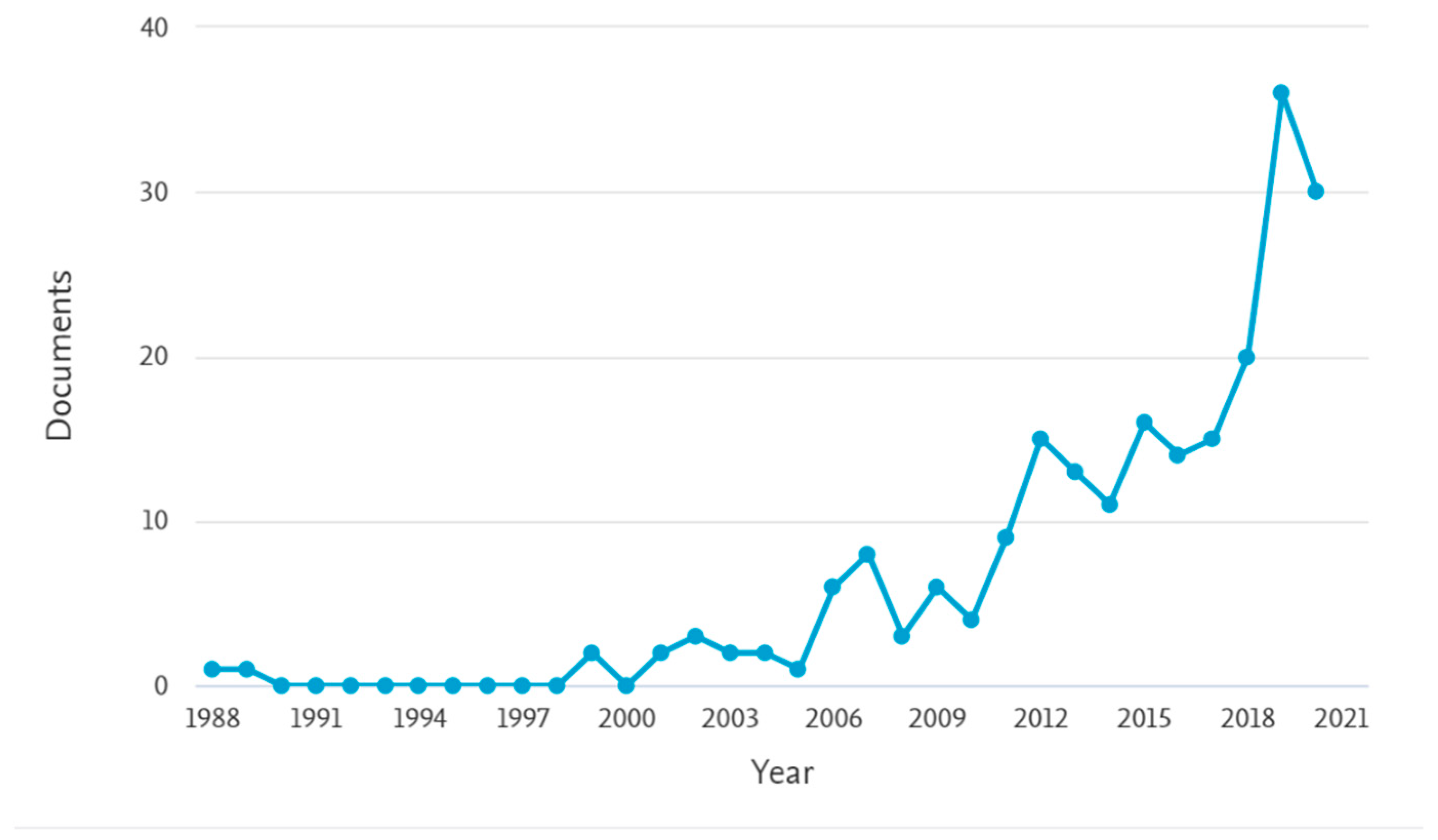
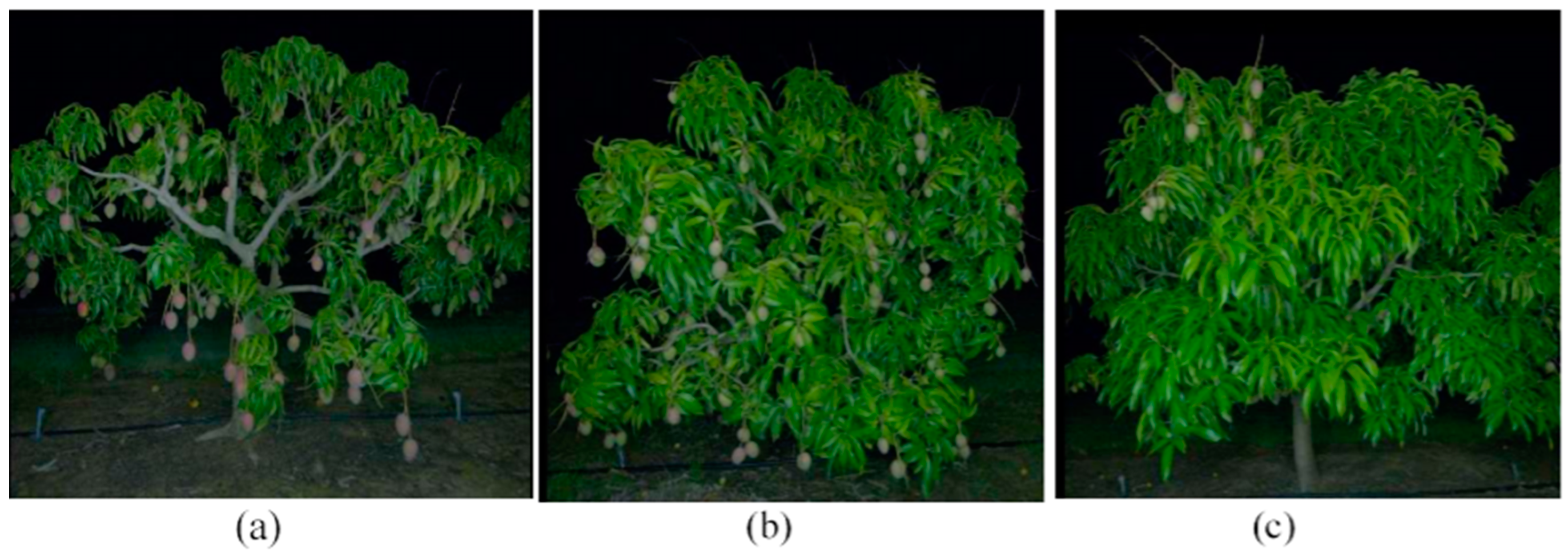
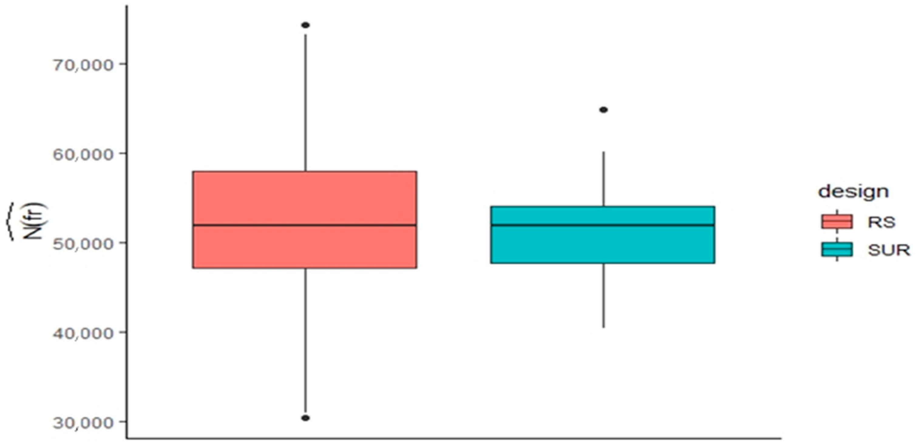
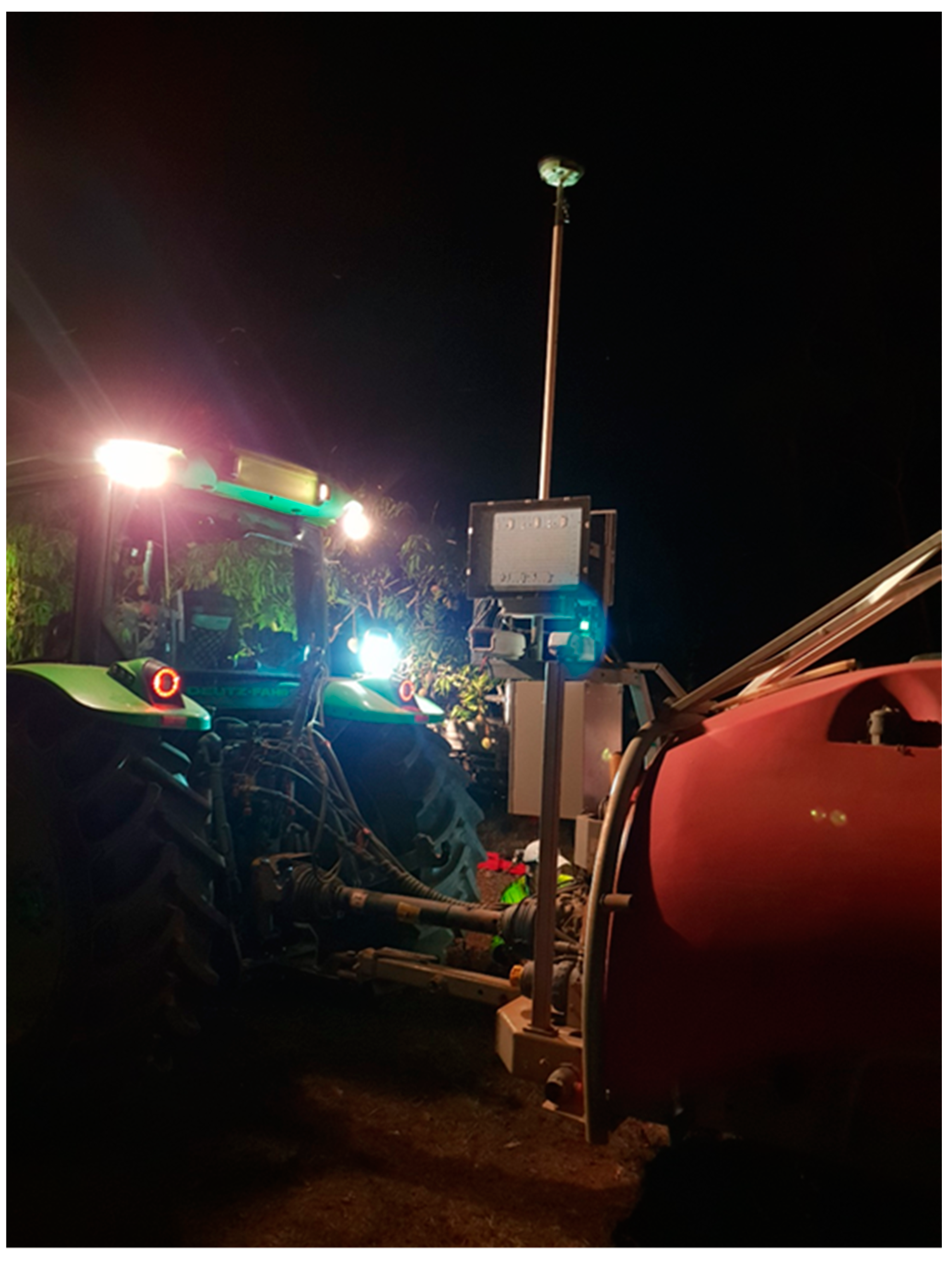
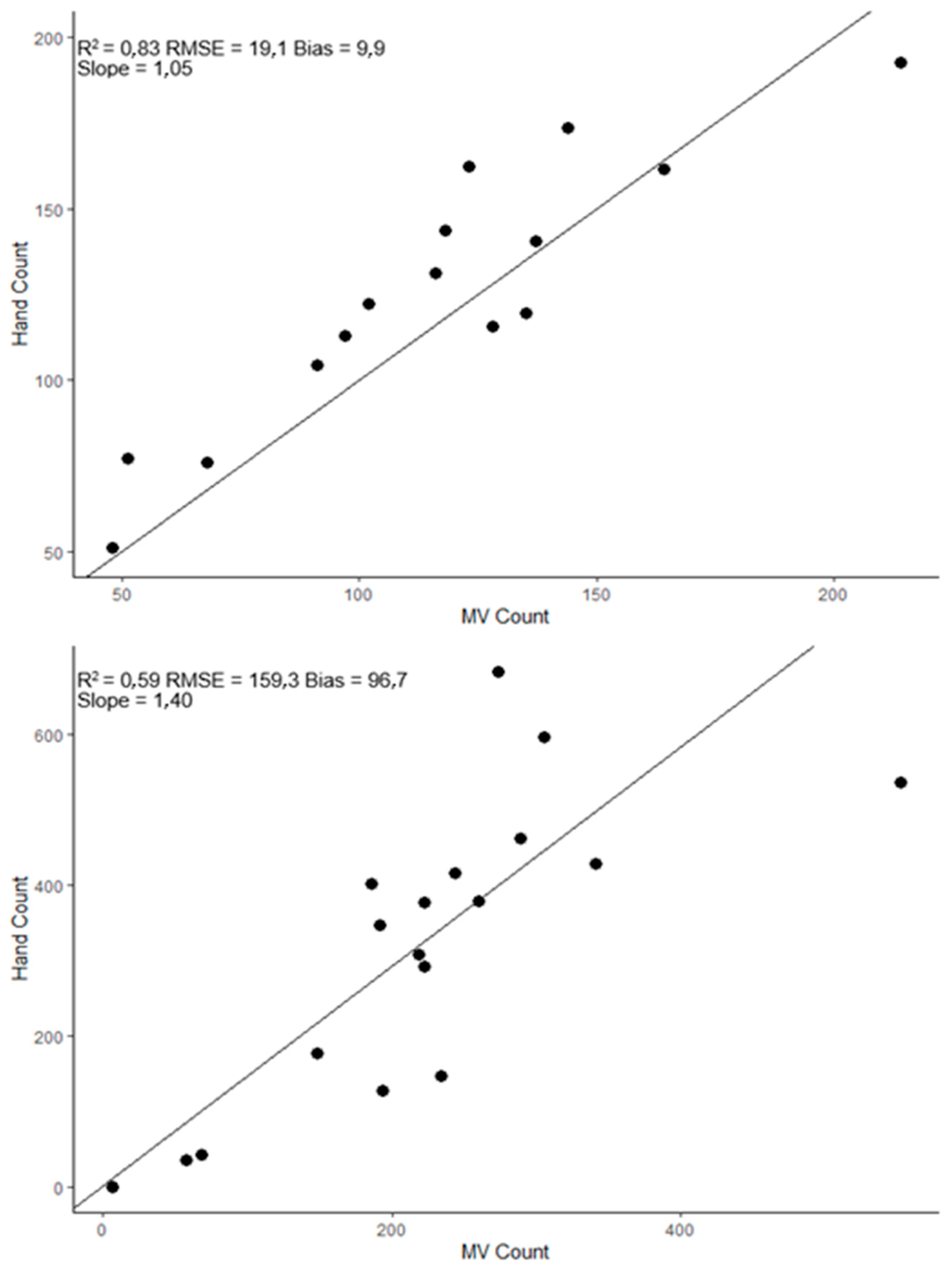
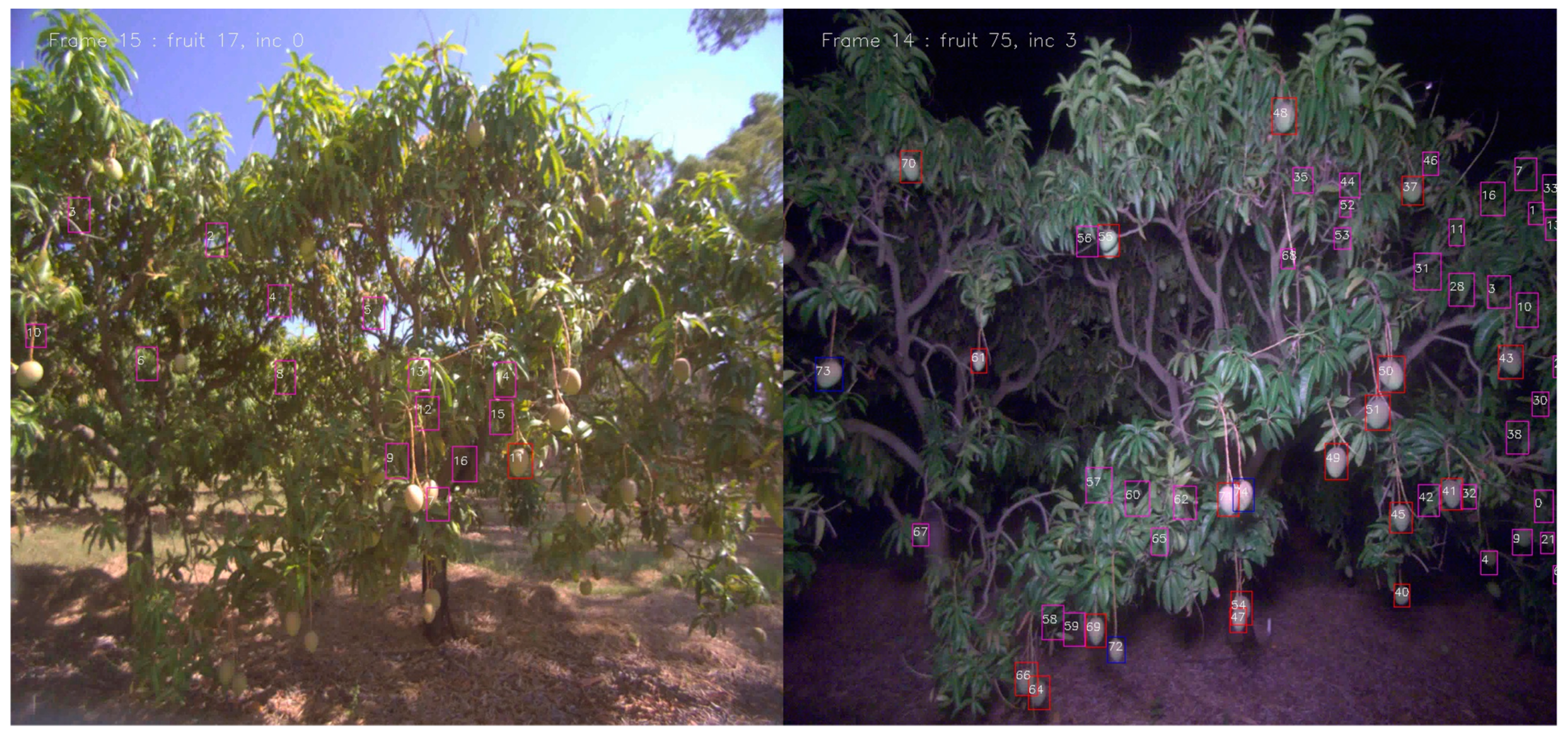
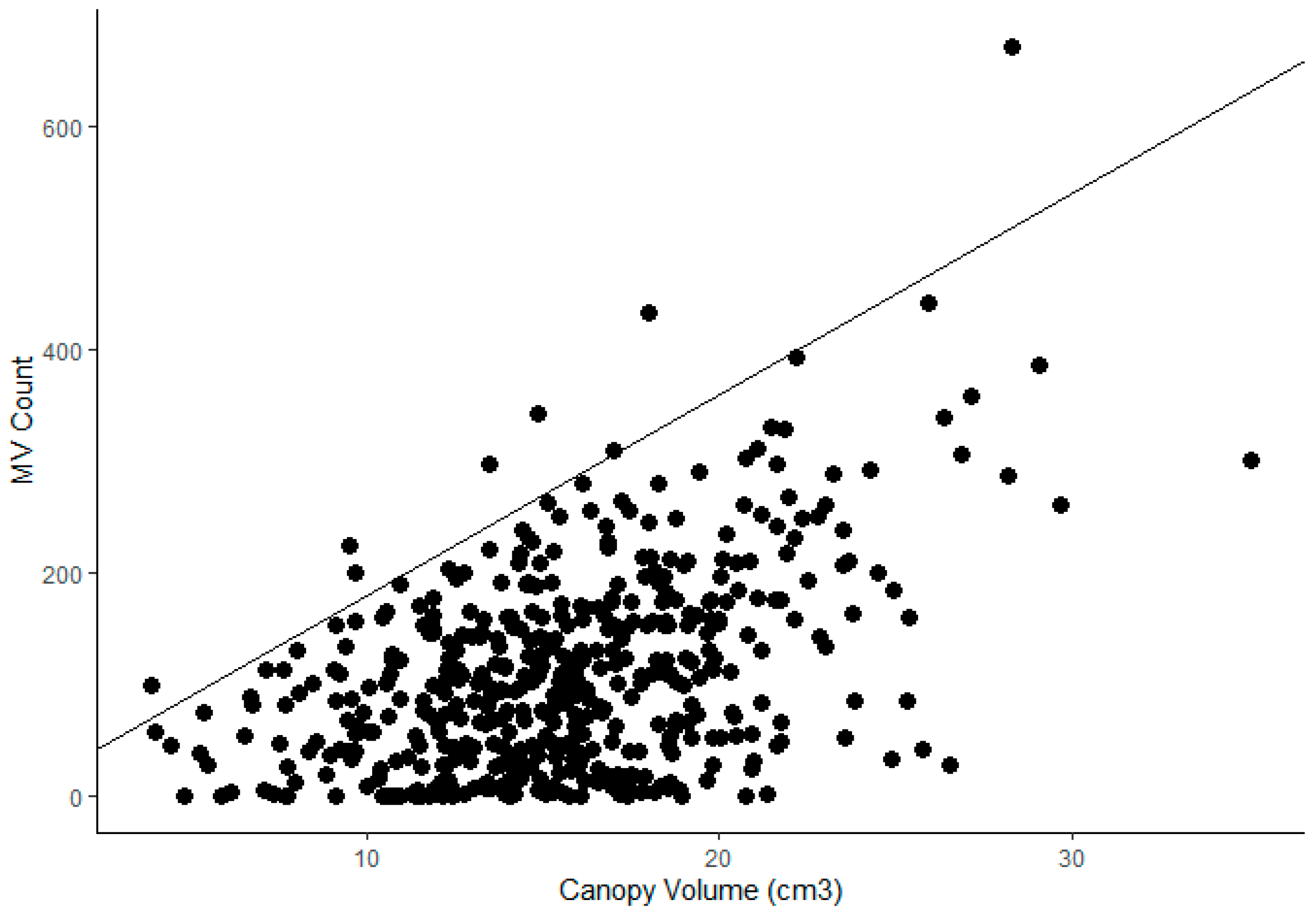
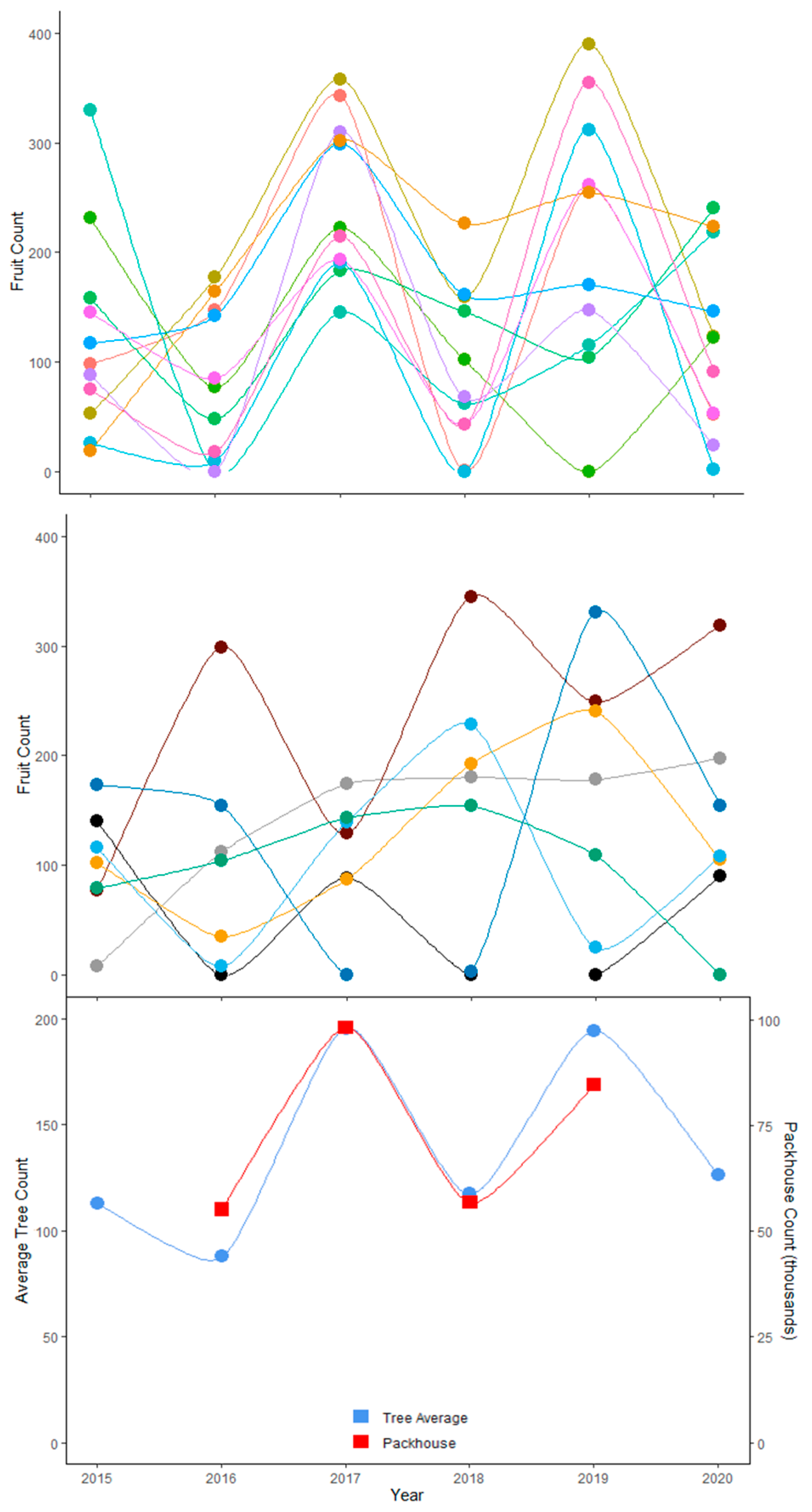
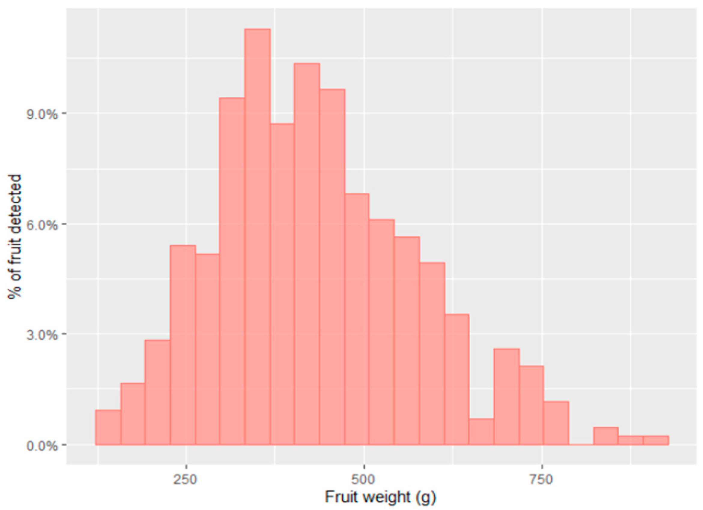
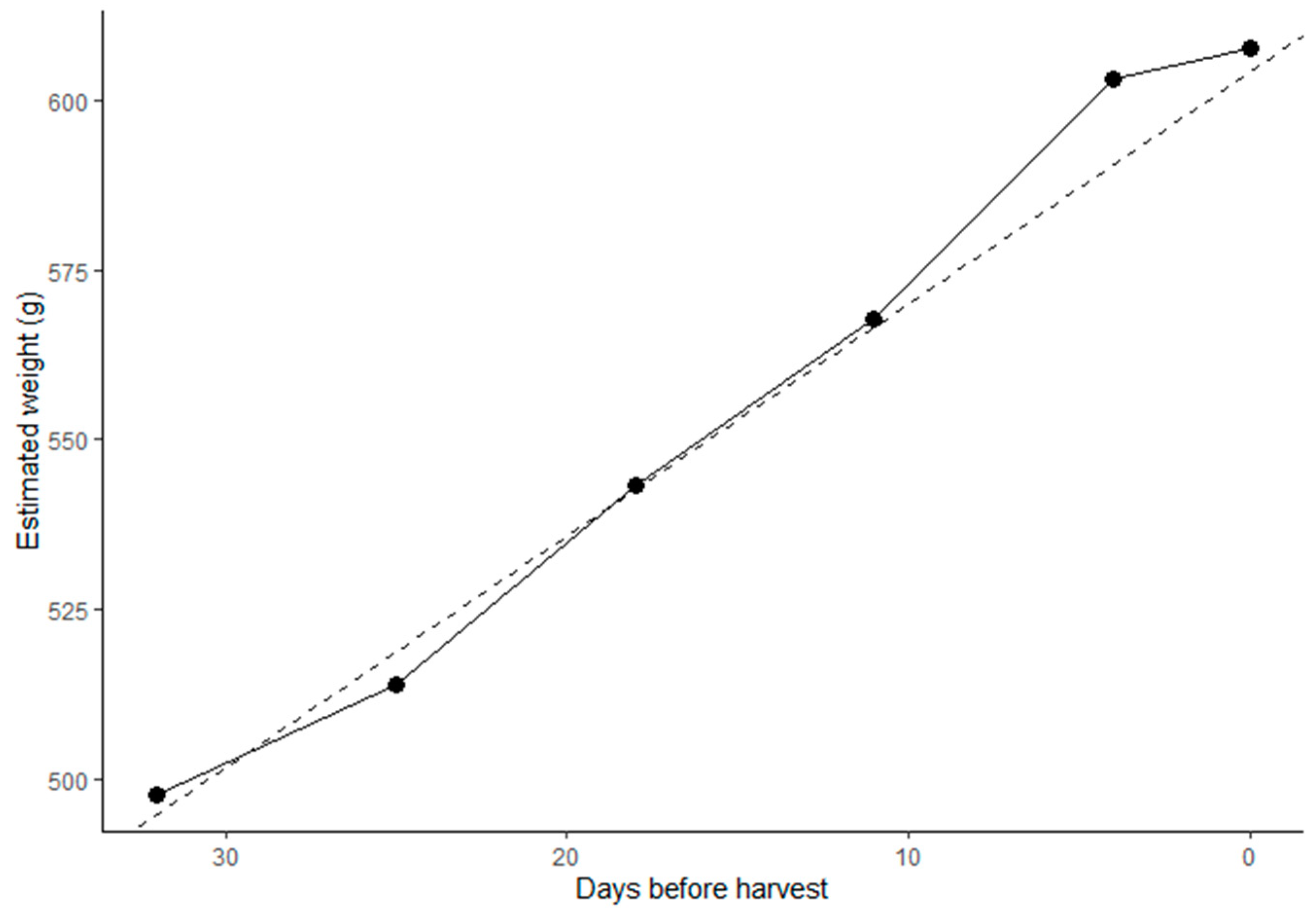
Table 1.
Literature base as indexed by Scopus records (doa 8/2/2021) for the keywords ‘fruit AND yield AND estimation’ for the years 2010–2021. # represents number.
Table 1.
Literature base as indexed by Scopus records (doa 8/2/2021) for the keywords ‘fruit AND yield AND estimation’ for the years 2010–2021. # represents number.
| Crop | # of Records | % | Country | # of Records | % |
|---|---|---|---|---|---|
| Apple | 32 | 33 | China | 38 | 21 |
| Mango | 19 | 20 | United States | 34 | 19 |
| Citrus | 17 | 18 | Spain | 29 | 16 |
| Other | 16 | 16 | Australia | 20 | 11 |
| Kiwi | 4 | 4 | India | 16 | 9 |
| Grape | 3 | 3 | Germany | 14 | 8 |
| Olive | 3 | 3 | Brazil | 11 | 6 |
| Tomato | 3 | 3 | France | 11 | 6 |
| Italy | 9 | 5 | |||
| Method | # of records | % | Estimation level | # of records | % |
| MV RGB | 65 | 59 | image | 36 | 38 |
| Satellite | 10 | 9 | tree | 28 | 30 |
| MV Hyperspectral | 8 | 7 | orchard | 19 | 20 |
| Proximal indirect | 8 | 7 | region | 11 | 12 |
| UAV | 7 | 6 | |||
| Historical/climate | 6 | 5 | |||
| Manual | 6 | 5 |
Table 2.
Definition of evaluation metrics.
| Term | Meaning | Equation |
|---|---|---|
| RMSE | The standard deviation of the prediction residuals | where is the estimated value, is the observed value and n is the sample size |
| RRMSE | RMSE relative to mean | |
| MSE | The average squared errors of prediction residuals | |
| R2 | The proportion of the variance of one variable that can be explained by the variance of the second variable | where is the mean of observed values |
| MAE | The average of the absolute values of prediction residuals | |
| MAPE | The average of the absolute values of prediction residuals divided by the actual values | |
| CCC | Interpreted similarly to R2, but used to compare two methods predictions or to measure repeatability of repeats of a single method | where represents the variability of either the observed value or another variable and and the variability and the mean of either the estimated value or another variable |
| RCV | The minimal significant difference between temporally different measurements | where is the quantile for the desired probability from a standard normal distribution |
| MCC | Measures the agreement of binary classifications | where TP is true positives, TN is true negatives, FP is false positives and FN is false negatives of binary classification |
Table 3.
Calculated sample sizes (Equation (3)) and adjusted sample size (Equation (4)) required for SRS with a 90% confidence and a PE of 10% based on an estimated from a preliminary sample taken from the population of trees. Data from Anderson et al. [16]. # represents number.
Table 3.
Calculated sample sizes (Equation (3)) and adjusted sample size (Equation (4)) required for SRS with a 90% confidence and a PE of 10% based on an estimated from a preliminary sample taken from the population of trees. Data from Anderson et al. [16]. # represents number.
| Site | (# Trees) | Average (# Fruit/Tree) | (# Fruit/Tree) | (# Trees) Equation (3) | (# Trees) Equation (4) | |
|---|---|---|---|---|---|---|
| 1 | 469 | 88 | 82 | 234 | 156 | 33 |
| 2 | 486 | 259 | 102 | 42 | 38 | 8 |
| 3 | 1017 | 240 | 160 | 120 | 107 | 11 |
| 4 | 1100 | 80 | 34 | 49 | 47 | 4 |
| 5 | 224 | 59 | 36 | 100 | 69 | 31 |
| 6 | 1205 | 97 | 65 | 121 | 110 | 9 |
| 7 | 1091 | 201 | 55 | 20 | 20 | 2 |
| 8 | 1818 | 106 | 51 | 62 | 60 | 3 |
| 9 | 1176 | 77 | 61 | 169 | 148 | 13 |
| 10 | 1115 | 85 | 40 | 60 | 57 | 5 |
Only half of the orchards required a sample size of 5% or less of the trees.
Table 4.
Example reported results of machine vision-based estimation of tree fruit load. Papers are ordered chronologically within commodities. Single view refers to collection of one image per tree and one row side only. Dual view (DV) refers to collection of one image per tree side from each interrow and multi view (MV) entails collection of several images in succession per tree side.
| Paper | Algorithm/Technique | Imaging Method | Validation Set | Result |
|---|---|---|---|---|
| Apple | ||||
| Gongal et al. [54] | Color and shape thresholding | DV on ground vehicle with row cover | 20 trees | 20% error on fruit in image, 18% error on fruits per tree |
| Bargoti and Underwood [58] | CNN | MV on ground vehicle, day imaging | 15 rows | 10.8% error on fruit counts per tree |
| Cheng et al. [53] | Color thresholding, neural network utilizing ancillary variables (foliage area, fruit area) | Single view on ground vehicle, day imaging | Multi season cross validations (2009–2011) 180 trees total. | 10.7 and 8.9% MAPE for estimations of fruit per tree after fruit drop and during ripening period, respectively |
| Linker [57] | Speeded Up Robust Features | DV (2014) and MV (2016 set) ground vehicle, night imaging | 10 grabs of 20 random trees (2014 and 2016 separately) | 2014: 4.8% error and 2016: 5.4% error (fruit/tree) |
| Kuznetsova et al. [59] | YOLOv3 | Single view on stationary platform | 552 images | 93% precision; 1% error on fruit count per image |
| Citrus | ||||
| Gan et al. [60] | FRCNN | Fusion of thermal and RGB, day imaging | 1658 images | 95.5% precision on fruit/image |
| Apolo-Apolo et al. [46] | FRCNN | DV on UAV | 20 trees, 3 seasons | 11.5, 4.3 and 5.8% error against harvested kg for 2016, 2017, and 2018, respectively |
| Grape | ||||
| Nuske et al. [52] | Shape, texture, color, occlusion correction | MV at 6 fps on ground vehicle; stereo camera for position | 1212 vines of 5 varieties on 4 trellis types, for 4 seasons. | 4% error in yield prediction with use of occlusion correction |
| Font et al. [55] | Color thresholding and area or volume modeling | Single view on ground vehicle | 25 bunches | 16–17% error on bunch weight. |
| Kiwifruit | ||||
| Wijethunga et al. [44] | Color thresholding | Single view on ground vehicle, night imaging | 78 gold 42 green images | 7.1 and 24.9% error for gold and green varieties, respectively, for fruit in image counts |
| Mango | ||||
| Stein et al. [37] | FRCNN | DV and MV on ground vehicle, day imaging | 16 trees | 1.4% error on fruit per tree (MV) |
| Qureshi et al. [56] | Texture and shape segmenting | DV ground vehicle, multiple light conditions | Multiple validations (10–74 trees) | Multiple validations from 0.5 to 40% error on fruit per tree estimate (mean = 18.6 and sd = 15.6%) |
| Anderson et al. [16] | FRCNN | DV and MV on ground vehicle, night imaging | 1 orchard | 9 and 6% error on packhouse count (DV and MV, respectively) |
| Koirala et al. [3] | MangoYOLOv3 | DV on ground vehicle; night imaging | 5 orchards | 3% error on packhouse count (5 orchards combined) |
Table 5.
Examples of allometric relations between fruit lineal dimensions and weight, and growth models for prediction of size at harvest, for several commodities. Abbreviations are: W, fruit weight (g) at a given time, e.g., W60 DAB; where DAB is days after full bloom; HW, weight of fruit at harvest (g), L, fruit length (mm), Wi, fruit width (mm), T, fruit thickness (mm).
| Publication | Commodity | Allometry between Weight and Lineal Dimensions | Prediction of Harvest Weight |
|---|---|---|---|
| Marini et al. [90] | Apple (Gala) | Quadratic W = 17.03 – (1.48 × d) + (0.046 × d2) R2 = 0.972 | Linear HW = −169.09 + (8.19 × W60 DAB) R2 = 0.79 |
| Lakso et al. [91] | Apple (Empire) | Linear 1.47 to 1.95 g/day | |
| Ortega-Farias et al. [92] | Apple (Granny Smith) | Logistic growth curve | |
| Verreynne [93] | Citrus (Navel Orange) | Linear 26.4 mm/day | |
| Ellis et al. [94] | Grape | Bayesian predicted double sigmoid growth curve | |
| Hall et al. [95] | Kiwifruit | Linear 0.42 mL/day from 50 DAB | |
| Spreer and Müller [96] | Mango (Chok Anan) | Linear W = 0.000539 × L × Wi × T R2 = 0.97 | |
| Wang et al. [97] | Mango (HoneyGold) | Linear W = 0.42 × L × Wi2 R2= 0.96 |
Publisher’s Note: MDPI stays neutral with regard to jurisdictional claims in published maps and institutional affiliations. |
© 2021 by the authors. Licensee MDPI, Basel, Switzerland. This article is an open access article distributed under the terms and conditions of the Creative Commons Attribution (CC BY) license (https://creativecommons.org/licenses/by/4.0/).
Share and Cite
MDPI and ACS Style
Anderson, N.T.; Walsh, K.B.; Wulfsohn, D. Technologies for Forecasting Tree Fruit Load and Harvest Timing—From Ground, Sky and Time. Agronomy 2021, 11, 1409. https://0-doi-org.brum.beds.ac.uk/10.3390/agronomy11071409
AMA Style
Anderson NT, Walsh KB, Wulfsohn D. Technologies for Forecasting Tree Fruit Load and Harvest Timing—From Ground, Sky and Time. Agronomy. 2021; 11(7):1409. https://0-doi-org.brum.beds.ac.uk/10.3390/agronomy11071409
Chicago/Turabian StyleAnderson, Nicholas Todd, Kerry Brian Walsh, and Dvoralai Wulfsohn. 2021. "Technologies for Forecasting Tree Fruit Load and Harvest Timing—From Ground, Sky and Time" Agronomy 11, no. 7: 1409. https://0-doi-org.brum.beds.ac.uk/10.3390/agronomy11071409
Note that from the first issue of 2016, this journal uses article numbers instead of page numbers. See further details here.