UAV-Based Hyperspectral and Ensemble Machine Learning for Predicting Yield in Winter Wheat

Abstract

Winter wheat is a widely-grown cereal crop worldwide. Using growth-stage information to estimate winter wheat yields in a timely manner is essential for accurate crop management and rapid decision-making in sustainable agriculture, and to increase productivity while reducing environmental impact. UAV remote sensing is widely used in precision agriculture due to its flexibility and increased spatial and spectral resolution. Hyperspectral data are used to model crop traits because of their ability to provide continuous rich spectral information and higher spectral fidelity. In this study, hyperspectral image data of the winter wheat crop canopy at the flowering and grain-filling stages was acquired by a low-altitude unmanned aerial vehicle (UAV), and machine learning was used to predict winter wheat yields. Specifically, a large number of spectral indices were extracted from the spectral data, and three feature selection methods, recursive feature elimination (RFE), Boruta feature selection, and the Pearson correlation coefficient (PCC), were used to filter high spectral indices in order to reduce the dimensionality of the data. Four major basic learner models, (1) support vector machine (SVM), (2) Gaussian process (GP), (3) linear ridge regression (LRR), and (4) random forest (RF), were also constructed, and an ensemble machine learning model was developed by combining the four base learner models. The results showed that the SVM yield prediction model, constructed on the basis of the preferred features, performed the best among the base learner models, with an R² between 0.62 and 0.73. The accuracy of the proposed ensemble learner model was higher than that of each base learner model; moreover, the R² (0.78) for the yield prediction model based on Boruta’s preferred characteristics was the highest at the grain-filling stage.

1. Introduction

Winter wheat is one of the three major cultivated cereals and is the most widely-grown cereal crop in the world [1]. Wheat plays a crucial role in global food production, trade, and food security [2]. Estimating wheat yield prior to harvest on a large scale not only offers a scientific foundation for local governments to establish production goals, but also ensures food security [3]. Therefore, the timely and accurate estimation of winter wheat yield is crucial for intelligent agricultural management and people’s livelihoods.

The traditional yield assessment of winter wheat involves destructive sampling in the field in order to determine yield, which is not only time consuming, less objective, and lacking in robustness and sustainability, but also fails to monitor the crop growth throughout its reproductive life [4]. The development of remote sensing technology in recent years has provided a non-destructive, rapid, and efficient way to monitor crop growth [5]. Remote sensing techniques include ground-based platforms, satellite-based platforms, and UAV-based platforms [6]. The data collection from the ground-based platforms requires a large amount of manpower and resources, the collection process can cause damage to the crop, and orthophotos of the crop cannot be obtained [7]. Satellite remote sensing, on the other hand, makes up for the shortcomings of the ground-based platforms and can monitor crops non-destructively and efficiently [8]. However, the satellite-based platform is more suitable for large-scale crop monitoring and may have some issues, such as low spatial and temporal resolution, long cycle time, and pixel mixing, which severely limit the quantitative assessment on a regional scale [9]. Unlike the satellite-based remote sensing, the low-altitude UAV remote sensing has the advantages of low cost, ease of operation, high efficiency, high spatial and temporal resolution, and flexibility. UAV-based remote sensing platforms that are equipped with various sensors can be used for water and fertilizer management in precision agriculture. [7,8]. UAV remote sensing has been widely used in agriculture for information acquisition and crop monitoring [9], although the flight of drones may sometimes require administrative authorization.

In recent years, many different types of sensors have been installed on UAV platforms for use in precision agriculture. Traditional RGB (red–green–blue) sensors with three bands are low-cost, relatively simple to process, and give high spatial resolution, and there has been a lot of research using these three bands or derived color indices, such as the green leaf algorithm index (GLA), to predict yields [10]. As a result of ongoing research, it has been found that plants often have strong reflectance properties in the near-infrared (NIR) band; therefore, multispectral cameras with NIR bands have received a lot of attention lately [11]. Vegetation indices, such as the ratio vegetation index (RVI), the normalized difference vegetation index (NDVI), and the canopy chlorophyll content index (CCCI), have been developed using NIR bands and have been successfully used for crop yield prediction, identification of soil salinity distribution, crop pest and disease monitoring, and the assessment of crop water and fertility status [12,13,14,15].

Hyperspectral cameras are known for their multiple wavelength bands, rich spectral information, high spectral resolution, and high recognition capability. Consequently, these cameras can acquire near-continuous spectral information of features for fast, nondestructive, and high-throughput detection of crops with large data volumes [16]. Therefore, hyperspectral images are widely used in precision agriculture, such as in the monitoring for pests and diseases, estimating crop biomass, and the monitoring of crop growth [17,18,19]. RGB images have red, green, and blue bands only, which are less informative and generally less accurate, and the accuracy of yield estimation models for winter wheat constructed using spectral parameters obtained from hyperspectral images is significantly higher than the accuracy of estimation models using RGB images [20]. For example, narrowband NDVI extracted from hyperspectral data explained more yield variability compared to multispectral data in sorghum yield prediction [21].

Typically, feature selection methods begin with a process of selecting a relevant subset of attributes in a dataset when developing a machine learning model, which can effectively avoid dimensional disasters, reduce the impact of noisy data with unknown irrelevant and redundant features on the prediction model, reduce computation time, improve the performance of the prediction model, and contribute to a better understanding of the dataset [22]. The Pearson correlation coefficient (PCC), a measure of linear correlation between variables, evaluates a subset of features through a proxy measure and is a filtering method for indirectly evaluating regression problems [23]. Wrapper methods are direct predictive models used to evaluate selected feature subsets and to find the best performing model by training the model for each subset. Boruta and RFE are popular wrapper methods in use today [24,25].

Machine learning algorithms are able to establish empirical relationships between independent and dependent variables and have the advantage of predicting yields without relying on individual crop-specific parameters [26]. Current machine learning algorithms that have been developed for crop yield prediction rely on a single predictive model [6,7,27]. Applying machine learning algorithms to training data with small sample sizes can have potential problems, such as bias, weak generalization, overfitting, and poor repeatability [26,28,29]. Most of the previous studies have focused on the mining of spectral information and the exploration of regression techniques based on machine learning algorithms [30,31], and there has been little discussion and research on model fusion. Therefore, the potential problems of small sample size and single machine learning algorithms can limit the application to winter wheat yield estimation in practical production. In order to address this issue, we introduced decision-level fusion (DLF) models in ensemble machine learning. The DLF models fuse multichannel/multiscale information and typically produce more consistent and better prediction performance than individual models, have good noise immunity, can handle high-dimensional data, provide complete and detailed object information, and are simple to implement and fast to train [32,33]. These models are extensively used in the fields of injury detection, artificial intelligence, and image processing [34,35,36]. Based on previous studies, machine learning and hyperspectral imagery have been used successfully in many applications, but the strategy based on DLF model fusion has not yet been applied to crop yield prediction [37,38].

The aim of this study was to estimate winter wheat yield using hyperspectral imagery from a UAV. The specific objectives included the following: (1) investigating the potential of hyperspectral imagery for winter wheat yield prediction, (2) evaluating the performance of winter wheat yield prediction models under different feature selection methods, and (3) building a DLF model based on individual machine learning algorithms in order to improve prediction performance.

2. Materials and Methods

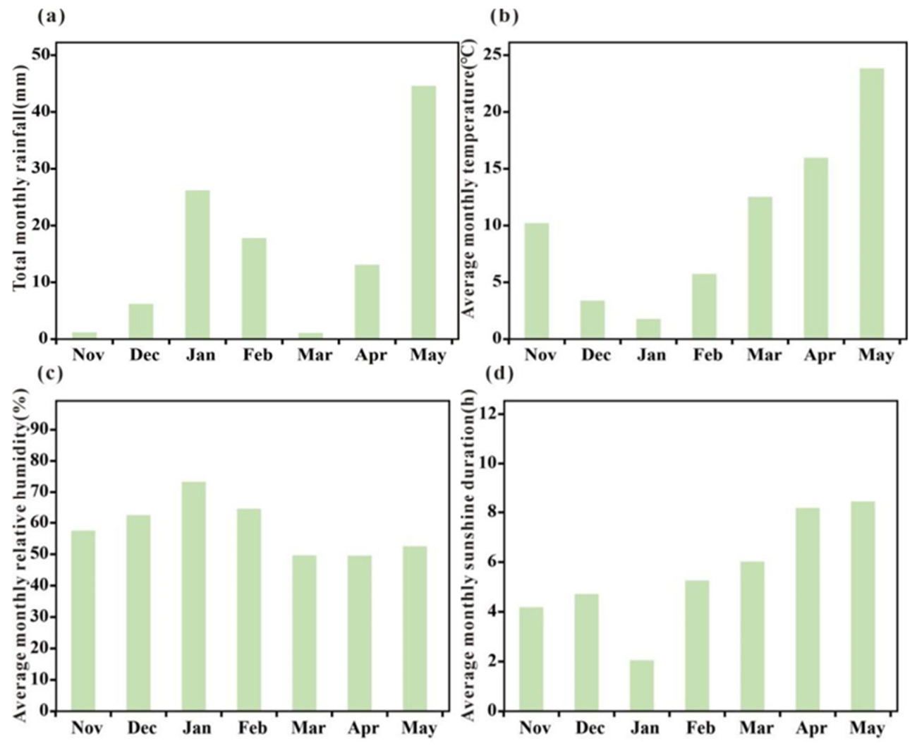
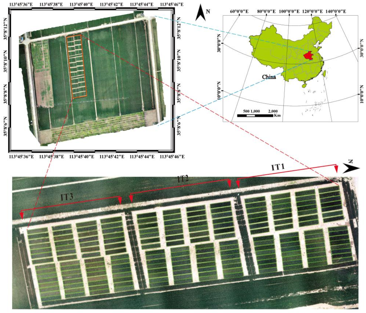
2.1. Experimental Design and Data Collection

This research trial was conducted in the 2019–2020 growing season at the experimental base of the Chinese Academy of Agricultural Sciences in Xinxiang, Henan Province (113°45′38″ N, 35°8′10″ E). During the winter wheat reproductive period (November 2019–June 2020), the total monthly rainfall, average monthly temperature, and average monthly sunshine hours all reached their maximums in May, while the monthly relative humidity reached its maximum in January (Figure 1). Rainfall was mainly concentrated in January, February, April, and May; temperature and sunshine hours both increased gradually from January onwards as the crop developed; and relative humidity was fairly constant throughout the season.

The trial area shown in Figure 2 consisted of 180 plots with three irrigation treatments set at high irrigation (irrigation treatment 1, IT1), moderate irrigation (irrigation treatment 2, IT2), and low irrigation (irrigation treatment 3, IT3) during the full growth period, using large sprinklers corresponding to a total irrigation water depth of 240 mm, 190 mm, and 145 mm, respectively. The irrigation schedule for each stage is shown in

Table 1. Summary of irrigation volumes for the three treatments at six stages of growth for winter wheat.

Growth Itage	High Irrigation (mm)	Moderate Irrigation (mm)	Low Irrigation (mm)
Tillering	35	35	35
Overwintering	35	35	35
Greening	35	25	20
Jointing	50	35	20
Heading	50	35	20
Grain filling	35	25	15
Total	240	190	145

. Each irrigation treatment had 60 plots, 8 m long and 1.4 m wide, with an area of 11.2 m². Thirty varieties of winter wheat were selected for this experiment, and each irrigation treatment was replicated twice in a group of 30 wheat varieties to ensure the objectivity of the experiment. For production fields, pesticide and fertilizer management was performed according to local management practices. At maturity (3 June 2020), winter wheat yields were collected using a plot combine.

2.2. Acquisition and Processing of Hyperspectral Data

The M600 Pro (SZ DJI Technology Co, Shenzhen, China) was used as the flight platform with an onboard Resonon Pika L nano-hyperspectral propulsion scanner to acquire hyperspectral data. The Resonon Pika L Nano-Hyperspec with meter-level accuracy is a lightweight (0.6 kg) hyperspectral sensor specifically designed for use on UAV platforms. This sensor has 300 spectral bands in the 400–1000 nm wavelength range with a band width of 2.1 nm, including the visible and near infrared regions. It is externally pushed and scanned with a choice of scanning angles (vertically downwards, horizontally, or at any angle). The Resonon Pika L Nano-Hyperspec features a focal length of 12 mm and offers a 22° field of view. Each scan line contains 640 pixels with a pixel pitch of 6 μm. The spectral resolution and resampling intervals are 6 nm and 2 nm, respectively. The sensor also includes a GPS/inertial measurement unit (GPS/IMU) navigation system, which enables the gathering of real-time altitude data from the UAV platform, allowing for better reflection calibration and geographic alignment. Depending on the environmental circumstances, certain criteria were established to fit the site size survey in this study. To ensure the quality of the data, hyperspectral data corresponding to the flowering (Zadok 65) and grain-filling (Zadok 85) stages of the wheat were acquired on 30 April 2020 and 13 May 2020, respectively. Both UAV flights were carried out between 10 a.m. and 2 p.m. in clear and cloudless weather conditions to minimize the effect of shadows. The UAV flew at a speed of 5 m/s at a height of 40 m, with a ground sampling distance of 2.5 cm. Three 0.25 m² reference panels that differed in brightness (95% white, 40% grey, and 5% black) were placed within the study area for postprocessing and measured with the spectrometer. In this study, 12 ground control points (GCPs) were evenly distributed across the field as precise georeferenced positions, and their centimeter-level positioning accuracy was obtained through the differential global positioning systems.

The acquired hyperspectral data was subjected to radiometric correction, atmospheric correction, and geometric correction. Hyperspectral images were acquired at an altitude of 50 m and under stable light conditions, so atmospheric correction was not required. SpectrononPro software (version 3.4.0, Resonon) was used for hyperspectral image correction. For hyperspectral radiometric corrections, empirical linear corrections were made using the measured images and field spectra of the wheat and reference panels. The hyperspectral image radiance data was converted to reflectance by the known reflectance of the white reference panel.

Three standard panels with different reflectance properties were placed in the flight area to derive the three parameters for atmospheric correction. Geographical correction used position and attitude parameters from the GPS/IMU and the relationship between the GPS/IMU and the imager. The parameters were converted between their respective coordinate systems. Noise in the image data can cause large differences at the beginning and end of the spectral range shown by the image and field spectra, so it is necessary to eliminate certain bands from the image data. The background (shadows and dirt) was eliminated from each plot by thresholding the NIR band at a wavelength of 800 nm. According to previous studies, vegetation usually has higher reflection values than the background in the NIR region, which is the reason behind our filtering method, setting the threshold at 30%, and removing noise bands below 440 nm and above 960 nm.

2.3. Acquisition of Spectral Indices

Hyperspectral data acquired using UAVs consists of hundreds of bands that contain a wealth of spectral information, and many of the adjacent bands are highly correlated with each other [39]. Sixty published spectral indices calculated using spectral reflectance were selected for predicting yield (

Table 2. Summary of the 60 spectral indices explored in this study.

Full Form	Spectral Index or Ratio	Formula	Application	Reference
Curvative index	CI	$\mathrm{R}675\times \mathrm{R}690/\mathrm{R}{683}^2$.	Chlorophyll	[40]
Chlorophyll index red-edge	CIre	$\mathrm{R}750/\mathrm{R}710-1$	Vegetation, chlorophyll	[41]
	Datt1	$\left(\mathrm{R}850-\mathrm{R}710\right)/\left(\mathrm{R}850-\mathrm{R}680\right)$	Vegetation, chlorophyll	[42]
	Datt4	$\mathrm{R}672/\left(\mathrm{R}550\times \mathrm{R}708\right)$
	Datt6	$\mathrm{R}860/\left(\mathrm{R}550\times \mathrm{R}708\right)$
Double difference index	DDI	$\left(\mathrm{R}749-\mathrm{R}720\right)-\left(\mathrm{R}701-\mathrm{R}672\right)$	Vegetation	[43]
Double peak index	DPI	$\left(\mathrm{R}688+\mathrm{R}710\right)/\mathrm{R}{697}^2$	Vegetation, chlorophyll	[44]
Gitelson2		$\left(\mathrm{R}750-\mathrm{R}800\right)/\left(\mathrm{R}695-\mathrm{R}740\right)-1$	Chlorophyll
Green normalized difference vegetation index	GNDVI	$\left(\mathrm{R}750-\mathrm{R}550\right)/\left(\mathrm{R}750+\mathrm{R}550\right)$	Vegetation, chlorophyll	[45]
Leaf chlorophyll index	LCI	$\left(\left|\mathrm{R}850| - |\mathrm{R}710\right|\right)/\left(\left|\mathrm{R}850| + |\mathrm{R}680\right|\right)$	Vegetation, chlorophyll	[46]
Modified chlorophyll absorption ratio index	MCARI	$\left[\left(\mathrm{R}700-\mathrm{R}670\right)-0.2\left(\mathrm{R}700-\mathrm{R}550\right)\right]\left(\mathrm{R}700/\mathrm{R}670\right)$	Vegetation, chlorophyll	[47]
	MCARI3	$[\left(\mathrm{R}750-\mathrm{R}710\right)-0.2(\mathrm{R}750-$$\mathrm{R}550\left)\right](\mathrm{R}750/\mathrm{R}715)$
Modified normalized difference	MND[680,800]	$\left(\mathrm{R}800-\mathrm{R}680\right)/\left(\mathrm{R}800+\mathrm{R}680-2\times \mathrm{R}445\right)$	Pigments	[48]
Modified normalized difference	MND[705,750]	$\left(\mathrm{R}750-\mathrm{R}705\right)/\left(\mathrm{R}750+\mathrm{R}705-2\times \mathrm{R}445\right)$
Modified simple ratio	mSR	$\left(\mathrm{R}800-\mathrm{R}445\right)/\left(\mathrm{R}680-\mathrm{R}445\right)$	Vegetation	[43]
Modified simple ratio 2	mSR2	$\left(\mathrm{R}750/\mathrm{R}705-1\right)/\left(\sqrt{\mathrm{R}750/\mathrm{R}705+1}\right)$		[44]
MERIS terrestrial chlorophyll index	MTCI	$\left(\mathrm{R}754-\mathrm{R}709\right)/\left(\mathrm{R}709-\mathrm{R}681\right)$	Vegetation, chlorophyll	[49]
Modified triangular vegetation index 1	MTVI1	$1.2\left[1.2\left(\mathrm{R}800-\mathrm{R}550\right)-2.5\left(\mathrm{R}670-\mathrm{R}550\right)\right]$	Vegetation	[50]
Modified triangular vegetation index 2	MTVI2	$\left(1.5\frac{1.2\left(\mathrm{R}800-\mathrm{R}550 \right)-2.5\left(\mathrm{R}670-\mathrm{R}550\right)}{\sqrt{\left(2\times \mathrm{R}800+1^2\right)-(6\times \mathrm{R}800-5\sqrt{\mathrm{R}670 )}-0.5}}\right)$
Normalized difference 550/531	ND[531,550]	$(\mathrm{R}550-\mathrm{R}531)/(\mathrm{R}550+\mathrm{R}531)$	Vegetation, chlorophyll	[44]
Normalized difference 682/553	ND[553,682]	(R682 − R553)/(R682 + R553)
Normalized difference chlorophyll	NDchl	(R925 − R710)/(R925 + R710)		[51]
New double difference index	DDn	$2\times \left(\mathrm{R}710-\mathrm{R}760-\mathrm{R}760\right)$	Chlorophyll
Normalized difference red-edge	NDRE	$\left(\mathrm{R}790-\mathrm{R}720\right)/\left(\mathrm{R}790+\mathrm{R}720\right)$	Vegetation	[52]
Normalized difference vegetation index	NDVI[650,750]	$\left(\mathrm{R}750-\mathrm{R}650\right)/\left(\mathrm{R}750+\mathrm{R}650\right)$	Vegetation, vitality	[53]
	NDVI[550,750]	$\left(\mathrm{R}750-\mathrm{R}550\right)/\left(\mathrm{R}750+\mathrm{R}550\right)$
	NDVI[710,750]	$\left(\mathrm{R}750-\mathrm{R}710\right)/\left(\mathrm{R}750+\mathrm{R}710\right)$
Normalized pigment chlorophyll index	NPCI	$(\mathrm{R}680-\mathrm{R}430)/(\mathrm{R}680+\mathrm{R}430)$	Vegetation, chlorophyll	[54]
Normalized difference pigment index	NPQI	(R415 − R435)/(R415 + R435)	Vegetation, chlorophyll	[55]
Optimized soil-adjusted vegetation index	OSAVI	$\left(1+0.16\right)\left(\mathrm{R}800-\mathrm{R}670\right)\left(\mathrm{R}800+\mathrm{R}670+0.16\right)$	Vegetation	[56]
Plant biochemical index	PBI	$\mathrm{R}810/\mathrm{R}560$	Vegetation	[57]
Plant pigment ratio	PPR	$\left(\mathrm{R}550-\mathrm{R}450\right)/\left(\mathrm{R}550+\mathrm{R}450\right)$	Vegetation	[58]
Physiological reflectance index	PRI	$\left(\mathrm{R}550-\mathrm{R}530\right)/\left(\mathrm{R}550+\mathrm{R}530\right)$	Vegetation	[59]
Pigment-specific normalized difference	PSNDb1	$\left(\mathrm{R}800-\mathrm{R}650\right)/\left(\mathrm{R}800+\mathrm{R}650\right)$	Vegetation, chlorophyll	[60]
	PSNDc1	$\left(\mathrm{R}800-\mathrm{R}500\right)/\left(\mathrm{R}800+\mathrm{R}500\right)$
	PSNDc2	$\left(\mathrm{R}800-\mathrm{R}470\right)/\left(\mathrm{R}800+\mathrm{R}470\right)$
Plant senescence reflectance index	PSRI	$\left(\mathrm{R}678-\mathrm{R}500\right)/\mathrm{R}750$	Vegetation	[61]
Pigment-specific simple ratio	PSSRc1	$\mathrm{R}800/\mathrm{R}500$	Vegetation, chlorophyll	[62]
	PSSRc2	$\mathrm{R}800/\mathrm{R}470$
Photosynthetic vigor ratio	PVR	$\left(\mathrm{R}550-\mathrm{R}650\right)/\left(\mathrm{R}550+\mathrm{R}650\right)$	Vegetation	[53]
Plant water index	PWI	$\mathrm{R}970/\mathrm{R}900$	Vegetation, water stress	[63]
Renormalized difference vegetation index	RDVI	$\left(\mathrm{R}800-\mathrm{R}670\right)/(\sqrt{\mathrm{R}800+\mathrm{R}670)}$	Vegetation	[64]
	RDVI2	$\left(\mathrm{R}833-\mathrm{R}658\right)/\left(\sqrt{\mathrm{R}833+\mathrm{R}658}\right)$
Reflectance at the inflexion point	Rre	$\left(\left|\mathrm{R}670| + |\mathrm{R}780\right|\right)/2$	Vegetation	[51]
Red-edge stress vegetation index	RVSI	$\left(\left(\mathrm{R}718+\mathrm{R}748\right)/2\right)-\mathrm{R}733$.	Vegetation	[65]
Soil-adjusted vegetation index	SAVI	$1.16\left(\left(\mathrm{R}800-\mathrm{R}670\right)/\left(\mathrm{R}800+\mathrm{R}670+0.16\right)\right)$	Vegetation	[66]
Structure intensive pigment index	SIPI	$\left(\mathrm{R}800-\mathrm{R}445\right)/\left(\mathrm{R}800-\mathrm{R}680\right)$.	Pigments	[46]
Spectral polygon vegetation index	SPVI	$0.4\left(3.7\left(\mathrm{R}800-\mathrm{R}670\right)-1.2\left|\mathrm{R}530-\mathrm{R}670\right|\right)$	Vegetation	[44]
Simple ratio	SR[430,680]	$\mathrm{R}430/\mathrm{R}680$	Vegetation	[67]
	SR[440,740]	$\mathrm{R}440/\mathrm{R}740$		[44]
	SR[550,672]	$\mathrm{R}550/\mathrm{R}672$
	SR[550,750]	$\mathrm{R}550/\mathrm{R}750$
Disease-water stress index 4	DSWI-4	$\mathrm{R}550/\mathrm{R}680$	Vegetation, water stress	[68]
Simple ratio pigment index	SRPI	$\mathrm{R}430/\mathrm{R}680$	Vegetation, chlorophyll	[69]
Transformed chlorophyll absorption ratio	TCARI	$3\left(\left(\mathrm{R}700-\mathrm{R}670\right)-0.2\left(\mathrm{R}700-\mathrm{R}550\right)\left(\mathrm{R}700/\mathrm{R}670\right)\right)$	Vegetation, chlorophyll	[45]
Triangular chlorophyll index	TCI	$1.2\left(\mathrm{R}700-\mathrm{R}550\right)-1.5\left(\mathrm{R}670-\mathrm{R}550\right)\times \sqrt{\mathrm{R}700/\mathrm{R}670}$	Vegetation, chlorophyll	[45]
Triangular vegetation index	TVI	$0.5\left(120\left(\mathrm{R}750-\mathrm{R}550\right)-200\left(\mathrm{R}670-\mathrm{R}550\right)\right)$	Vegetation	[69]
Water band index	WBI	$\mathrm{R}970/\mathrm{R}902$	Vegetation, water stress	[70]
Combined MCARI/MTVI2	MCARI/MTVI2	$\mathrm{MCARI}/\mathrm{MTVI}2$	Vegetation, chlorophyll	[45]
Combined TCARI/OSAVI	TCARI/OSAVI	$\mathrm{TCARI}/\mathrm{OSAVI}$	Vegetation, chlorophyll	[56]

), with each spectral index derived from two or more spectral bands. These spectral indices included the curvative index (CI), chlorophyll absorption index (CAI), normalized difference vegetation index (NDVI), simple ratio index (SR), pigment-specific normalized difference (Psnd), renormalized difference vegetation index (RDVI), triangular vegetation index (TVI), modified versions of these indices, such as the modified normalized difference (MND), modified simple ratio (MSR), normalized difference (ND), and their combinations MCARI/ MTVI2, among others. The majority of the bands utilized are in the red, NIR, and red-edge spectral regions.

2.4. Feature Selection Methods

The choice of input features is as important as the choice of the algorithm to be used when building the model. In supervised learning, feature selection is often used prior to model development to minimize the feature set dimensionality and thus gain performance improvements in the learning algorithm. In this study, 60 spectral indices were chosen, so it was ideal to select the most sensitive spectral indices to reduce the number of features. The following three common feature selection methods were used in this study to rank the importance of features: recursive feature elimination (RFE), Boruta, and the Pearson correlation coefficient (PCC).

Recursive feature elimination (RFE) [71] is a wrapper-based feature selection method that selects features with the help of a classification method. RFE requires training multiple classifiers to reduce the feature dimension, training time increases with the number of classifiers trained, and each part of the analysis can continue to be iterated, saving computational time. Low-weighted features are eliminated in each iteration, while equal weights are assigned to relevant attributes. RCE is performed in three steps, as follows: (1) an estimator is used to estimate the initial features’ importance scores, (2) the feature with the lowest significance score is eliminated, and (3) a rank in given to each deleted variable in the order in which it was removed.

The Boruta [72] algorithm is a wrapper method built around the random forest algorithm. It provides criteria for a number of important factors and captures the outcome variables for all relevant features in the dataset by scoring all candidate features as well as shaded features. The importance value of the shaded features depends on whether the candidate features are significantly correlated or not. The Boruta algorithm steps are as follows: (1) randomly disrupt the feature order to obtain the shadow feature matrix, (2) train the model with the shadow feature matrix as input, (3) take the maximum value in the shadow features and record the cumulative hits of the real features to mark the features as important or unimportant, and (4) remove the unimportant features and repeat the first three steps until all the features are marked.

The Pearson correlation coefficient (PCC) [73] is a measure of the correlation between two variables, and it varies between −1 and 1. The PCC(r_xy) may be calculated using the following equation:

$$r_{xy}=\frac{{{\displaystyle \sum }}_{i=1}^n\left(x_i-\overline{x}\right){{\displaystyle \sum }}_{i=1}^n\left(y_i-\overline{y}\right)}{\sqrt{{{\displaystyle \sum }}_{i=1}^n{\left(x_i-\overline{x}\right)}^2}\sqrt{{{\displaystyle \sum }}_{i=1}^n{\left(y_i-\overline{y}\right)}^2}}$$

(1)

where $\overline{x }=\frac{1}{n}{\displaystyle \sum }_{i=1}^n{x}_i$ and $\overline{y}=\frac{1}{y}{\displaystyle \sum }_{i=1}^n{y}_i$ denote the means of x and y, respectively, with n representing the sample size. The PCC is invariant to both linear and non-linear changes of the variables. The absolute value of PCC was used to compute the feature significance scores.

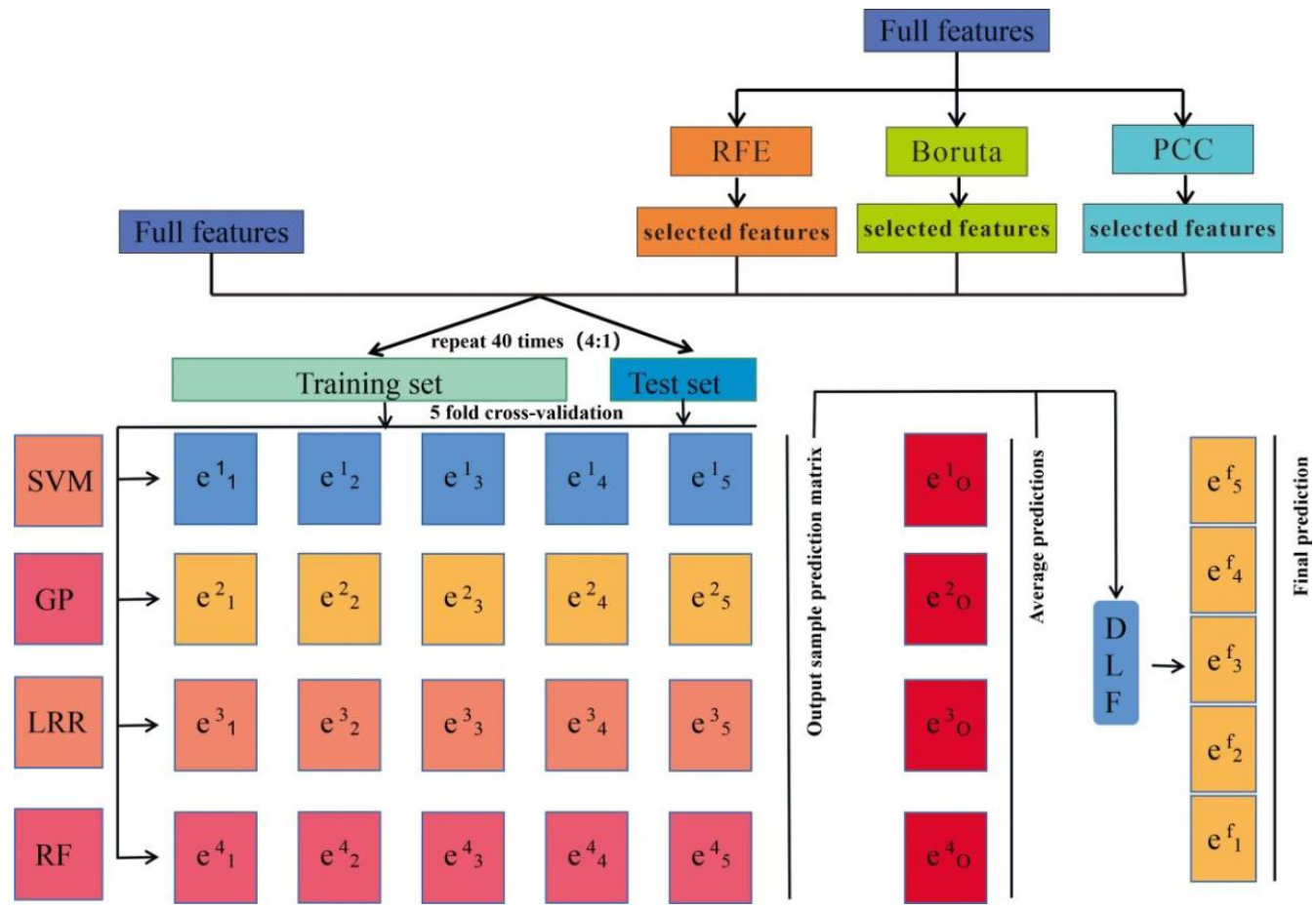
2.5. Decision-Level Fusion Model for Ensemble Learning

In this study, support vector machines (SVM), Gaussian process (GP), linear ridge regression (LRR), and random forest (RF) were the four regression models based on DLF for ensemble learning. The ‘caret’ R package in R4.0.2 was used to build the individual learner and DLF framework. The basic principle of DLF is shown in Figure 3. The hyperspectral index and winter wheat yield data pairs from 180 plots were randomly and uniformly divided into five groups, one group of which (n = 36) was randomly taken as the validation set and the remaining four groups (n = 144) as the training set. Predictions were made for each fold by training the model and five-fold cross-validation. In the five-fold cross-validation process, the winter wheat yield predictions were generated separately for each regression model, and the model effects could be observed by examining the results of the individual learners on the validation set. The m individual learners would get a prediction matrix of m × n dimensions after completing the above process (n was the number of samples in the training set and m was the number of individual learners), and the results of the prediction matrix were then used to train the DLF model to make the final prediction. Importantly, a five-fold cross-validation method was used in all of the models to ensure the reasonableness of the comparison between methods. To avoid uncertainty in the results, the process of dividing the data into training and validation sets using the five-fold cross-validation method was repeated 40 times to generate 200 models, and the mean prediction accuracy of the validation set of these 200 models was used as the final evaluation metric.

2.5.1. Regression Methods

Based on a survey of previous research, and in order to assess the effectiveness of different machine learning algorithms and to better comprehend the non-linear connection between the dependent and independent variables, the following four widely utilized machine learning models were selected and used for comparison: SVM, GP, LRR, and RF. The four machine learning algorithms are described below, as follows:

SVMs (support vector machines) [74], which benefit from statistical learning theory and the principle of minimal structural risk, are sparse and robust classifiers, mainly used for the classification and regression of high-dimensional samples. SVMs are increasingly popular in existing research areas because of their characteristics, such as good generalization ability and robustness to noise. SVMs are trained on sufficient samples in order to obtain a set of samples that approximate the hyperplane by fitting estimates of successive optimal output variables. The hyperplane is approximated by two important parameters, the kernel function and the loss function. The radial basis function was utilized as the kernel function in this research to change the regularization parameters using a cross-validation method.

GP (Gaussian process) [75] is a supervised learning process for estimating regression model parameters through sample learning. GP belongs to the stochastic process in probability theory and mathematical statistics, where any linear combination of random variables conforms to a normal distribution. GP is now widely used in modelling in the field of remote sensing, and therefore this algorithm was used in this study.

LRR (linear ridge regression) [76] is a biased estimation regression method dedicated to covariance data analysis. LRR obtains more objective regression coefficients by losing some information and reducing precision. Typically, LRR has a low R² and high regression coefficients, and is widely used in co-linear problems and research with a large amount of data. The LRR algorithm was used in this study to construct yield estimation models.

RF (random forest) [76] is an ensemble learning method that constructs multiple decision trees and can perform decision making and regression. RF is able to model the relationship between dependent and independent variables based on decision rules. It can handle a large number of input variables, assess the importance of variables while deciding on categories, produce higher accuracy, balance errors, and quickly mine the data. Therefore, the RF algorithm was used for modelling in this study.

The machine learning algorithms used in this study were all implemented independently. To improve the prediction accuracy of the models, we further processed these results to construct a DLF model [77], which is a model that fuses the results of different machine learning models by the training weights obtained. Based on previous research, a weighted prior (WP) approach was introduced to construct the DLF model, taking into account the estimated variance of each model. The DLF and WP can further improve the model accuracy and generalization ability and minimize the result bias. The procedure for this method is as follows [78]:

$${\epsilon }^{\left(i\right)}=y^{\left(i\right)}-y$$

(2)

where ${\epsilon }^{\left(i\right)}$ is the estimation variance,$y^{\left(i\right)}$ is the predicted value from the $i^{th}$ model, and $\mathrm{y}$ is the observed value.

$$var({\epsilon }^i)=\frac{1}{n}{\displaystyle \sum }_{j=1}^n({\epsilon }_j^{\left(i\right)}-\frac{1}{N}{\displaystyle \sum }_{j=1}^N{\epsilon }_J^{\left(i\right)}{)}^2$$

(3)

where N is the total number of samples in the training set.

$$w_i=\frac{1/var\left({\epsilon }^{\left(i\right)}\right)}{{{\displaystyle \sum }}_{k=1}^{l}1/var\left({\epsilon }^{\left(k\right)}\right)}$$

(4)

where $\mathrm{l}$ denotes the total number of models and $w_i$ denotes the weight of the $i^{th}$ model.

$$w_i^{\ast }=r{W}_i+\left(1-r\right)w_i$$

(5)

where $w_i^{\ast }$ is the final DLF weighting.

$$y^{\left(WP\right)}={\displaystyle \sum }_{i=1}^l{w}_i^{\ast }{y}^{\left(i\right)}$$

(6)

where $y^{WP}$ is the final result based on the WP method.

The individual machine learning models were used as input to build the DLF model.

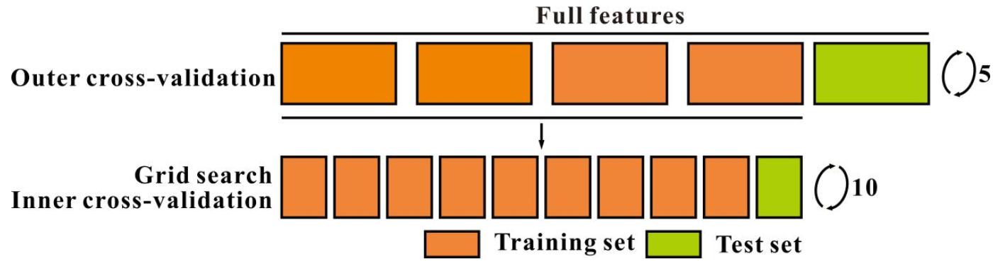
2.5.2. Cross-Validation and Parameter Optimization

A five-fold cross-validation was used to form the prediction matrix in the personal machine learning process of the DLF, which can be used as external cross-validation. In addition, internal random grid search cross-validation allows the fine-tuning of the hyperparameters of the individual learner shown in Figure 4. In external cross-validation, the original dataset is randomly divided into five equal parts (Figure 4), one of which is then used as the validation set and the remaining four as the training set each time. Each training set used for external cross-validation was also randomly divided into five equal parts, of which 1/5 was used as the validation set for internal cross-validation and the remaining 4/5 was used as the training set for internal cross-validation. The model was trained by setting different combinations of candidate hyperparameters for internal cross-validation, and the model was then validated on the internal cross-validation set. Each hyperparameter combination was validated five times, and after training model evaluation, the hyperparameter combination with the highest average validation accuracy was applied to the outer cross-validation to construct the ideal model.

2.6. Statistical Analysis

In this study, the regression model was evaluated in the four following ways: coefficient of determination (R²), root mean square error (RMSE), ratio of performance to interquartile distance (RPIQ), and ratio of performance to deviation (RPD). The criteria for evaluating models are yield estimation models with higher accuracy, and an RPD of >1.5 is usually considered to indicate a reliable prediction. The formulae for the four evaluation methods are as follows:

$${\mathrm{R}}^2=1-\frac{{{\displaystyle \sum }}_{i=1}^n{\left(\widehat{y_i}-y_i\right)}^2}{{{\displaystyle \sum }}_{i=1}^n{\left(y_i-\overline{y}\right)}^2}$$

(7)

$$\mathrm{RMSE}=\sqrt{\frac{{{\displaystyle \sum }}_{i=1}^n{\left(\widehat{y_i}-y_i\right)}^2}{\mathrm{N}}}$$

(8)

$$\mathrm{RPD}=\frac{\mathrm{SD}}{{\mathrm{RMSE}}_{\mathrm{p}}}$$

(9)

$$\mathrm{RPIQ}=\frac{{\mathrm{Q}}_3-{\mathrm{Q}}_1}{{\mathrm{RMSE}}_{\mathrm{p}}}$$

(10)

where $y_i$ is the measured value, $\widehat{y_i}$ is the predicted value, $\overline{y}$ is the mean of the measured values, N is the sample size, SD is the standard deviation of the measured value of the prediction set, $Q_3$ is the lower boundary of the third quartile, and $Q_1$ is the upper boundary of the first quartile.

3. Results

3.1. Descriptive Statistics

The yield of winter wheat in all of the test plots in this study was 6.55 t·ha⁻¹, and the mean yields differed for the three irrigation treatments. The yield statistics for the test plots under each irrigation treatment and all of the plots are shown in

Table 3. Descriptive statistics for the data sets from all test plots and the test plots from the three different irrigation treatments (t·ha⁻¹).

Category	N	Mean	SD	Min	Q25	Q50	Q75	Max	CV
All datasets	180	6.55	1.59	3.13	5.27	6.65	7.71	9.71	24.33%
IT1 dataset	60	7.97	1.01	5.58	7.43	7.97	8.65	9.71	12.68%
IT2 dataset	60	6.73	1.02	4.28	6.08	6.75	7.55	8.75	15.16%
IT3 dataset	60	4.94	0.96	3.13	4.31	4.89	5.55	7.54	19.50%

SD: standard deviation; Q25: lower quartile; Q50: median quartile; Q75: upper quartile; and CV: coefficient of variation.

. In general, the treatments with higher irrigation levels were associated with higher yields. IT1 had the highest average yield of 7.97 t·ha⁻¹, followed by IT2 at 6.73 t·ha⁻¹, and IT3 at 4.94 t·ha⁻¹. The data ranges, quantile statistics, standard deviations (SD), and coefficients of variation (CV) for the yield datasets for all of the plots and the three experimental treatments showed significant yield differences between the treatments and well separated datasets.

The simple linear regression coefficients of determination for each vegetation index at the flowering and the grain-filling stages are shown in

Table A1. The coefficients of determination for the 60 spectral indices under simple linear regression.

Full Form	Spectral Index or Ratio	R2
		Flowering	Grain Filling
Curvative index	CI	0.08	0.33
Chlorophyll index red-edge	CIre	0.21	0.40
	Datt1	0.30	0.31
	Datt4	0.14	0.41
	Datt6	0.05	0.29
Double difference index	DDI	0.24	0.26
Double peak index	DPI	0.14	0.30
Gitelson2		$0.21$	0.45
Green normalized difference vegetation index	GNDVI	$0.21$	0.40
Leaf chlorophyll index	LCI	$0.20$	0.42
Modified chlorophyll absorption ratio index	MCARI	$0.17$	0.41
	MCARI3	$0.22$	0.43
Modified normalized difference	MND[680,800]	$0.26$	0.45
Modified normalized difference	MND[705,750]	$0.20$	0.43
Modified simple ratio	mSR	$0.22$	0.32
Modified simple ratio 2	mSR2	$0.23$	0.41
MERIS terrestrial chlorophyll index	MTCI	$0.13$	0.31
Modified triangular vegetation index 1	MTVI1	$0.43$	0.40
Modified triangular vegetation index 2	MTVI2	$0.36$	0.47
Normalized difference 550/531	ND[531,550]	$0.13$	0.28
Normalized difference 682/553	ND[553,682]	0.41	0.48
Normalized difference chlorophyll	NDchl	0.23	0.36
New double difference index	DDn	0.45	0.39
Normalized difference red-edge	NDRE	$0.18$	0.36
Normalized difference vegetation index	NDVI[650,750]	$0.32$	0.47
	NDVI[550,750]	$0.23$	0.42
	NDVI[710,750]	$0.22$	0.43
Normalized pigment chlorophyll index	NPCI	$0.17$	0.35
Normalized difference pigment index	NPQI	0.13	0.31
Optimized soil-adjusted vegetation index	OSAVI	0.31	0.48
Plant biochemical index	PBI	0.20	0.37
Plant pigment ratio	PPR	0.09	0.25
Physiological reflectance index	PRI	0.40	0.48
Pigment-specific normalized difference	PSNDb1	0.31	0.46
	PSNDc1	0.28	0.44
	PSNDc2	$0.26$	0.43
Plant senescence reflectance index	PSRI	$0.24$	0.31
Pigment-pecific simple ratio	PSSRc1	$0.26$	0.39
	PSSRc2	$0.24$	0.38
Photosynthetic vigor ratio	PVR	$0.40$	0.48
Plant water index	PWI	$0.15$	0.28
Renormalized difference vegetation index	RDVI	$0.43$	0.44
	RDVI2	$0.42$	0.44
Reflectance at the inflexion point	Rre	$0.35$	0.14
Red-edge stress vegetation index	RVSI	$0.48$	0.49
Soil-adjusted vegetation index	SAVI	$0.31$	0.47
Structure intensive pigment index	SIPI	$0.44$	0.35
Spectral polygon vegetation index	SPVI	$0.44$	0.40
Simple ratio	SR[430,680]	$0.17$	0.34
	SR[440,740]	$0.31$	0.46
	SR[550,672]	$0.02$	0.25
	SR[550,750]	$0.01$	0.05
Disease-water stress index 4	DSWI-4	$0.43$	0.47
Simple ratio pigment index	SRPI	$0.17$	0.34
Transformed chlorophyll absorption ratio	TCARI	$0.01$	0.34
Triangular chlorophyll index	TCI	$0.08$	0.40
Triangular vegetation index	TVI	$0.43$	0.42
Water band index	WBI	$0.30$	0.31
Combined MCARI/MTVI2	MCARI/MTVI2	$0.13$	0.39
Combined TCARI/OSAVI	TCARI/OSAVI	$0.03$	0.10

. The results show that the R² of each spectral index in the grain-filling stage was mostly greater than that in the flowering stage. The RVSI index performed best at both stages, with R² values of 0.48 at the flowering stage, and 0.49 at the grain-filling stage. The poorest performing index was CI in the flowering stage, with an R² of 0.08, and the index with the poorest performance in the grain-filling stage was TCARI/OSAVI, with an R² of 0.1.

3.2. Feature Importance Ranking

In this study, RFE, Boruta, and PCC methods were used to rank the importance of 60 vegetation indices at the flowering and grain-filling stages. The results of the ranking of the importance of each vegetation index are shown in

Table A2. Ranking of all 60 features for the three feature selection methods at the flowering and grain-filling stages of winter wheat.

Ranking	Flowering Features			Grain-Filling Features
	RFE	Boruta	PCC	RFE	Boruta	PCC
1	RVSI	Gitelson2	RVSI	DSWI-4	Gitelson2	RVSI
2	RDVI	RVSI	DDn	ND[553,682]	RVSI	ND[553,682]
3	WBI	NDchl	SPVI	MTVI2	NDchl	PVR
4	NDVI[650,750]	ND[553,682]	SIPI	RVSI	ND[553,682]	OSAVI
5	PRI	OSAVI	MTVI1	Gitelson2	OSAVI	PRI
6	PWI	CIre	RDVI	PVR	CIre	NDVI[650,750]
7	DSWI-4	NDVI[710,750]	DSWI-4	CI	NDVI[710,750]	MTVI2
8	SR[440,740]	DPI	TVI	OSAVI	DPI	DSWI-4
9	SAVI	MSR2	RDVI2	NDchl	MSR2	SAVI
10	TCI	MTCI	ND[553,682]	Datt1	MTCI	SR[440,740]
11	MTVI1	DSWI-4	PRI	SR[450,550]	DSWI-4	PSNDb1
12	OSAVI	MND[705,750]	PVR	PPR	MND[705,750]	MND[680,800]
13	Datt4	MTVI2	MTVI2	CIre	MTVI2	Gitelson2
14	MSR	PVR	Rre	PRI	PVR	RDVI2
15	DDn	NDVI[650,750]	NDVI[650,750]	NPQI	NDVI[650,750]	RDVI
16	RDVI2	SAVI	SR[440,740]	SR[450,690]	SAVI	PSNDc1
17	MCARI	PRI	PSNDb1	Rre	PRI	MND[705,750]
18	ND[553,682]	Datt6	OSAVI	MSR2	Datt6	PSNDc2
19	PSNDb1	SR[440,740]	SAVI	TCARI/OSAVI	SR[440,740]	NDVI[710,750]
20	SIPI	DDI	WBI	DDI	DDI	MCARI3
21	Rre	PSNDb1	PSNDc1	MCARI	PSNDb1	NDVI[550,750]
22	TVI	LCI	PSNDc2	PSRI	LCI	LCI
23	Gitelson2	MND[680,800]	MND[680,800]	LCI	MND[680,800]	TVI
24	Datt1	NDRE	PSSRc1	Datt4	NDRE	MSR2
25	NDchl	PSSRc1	DDI	MCARI/MTVI2	PSSRc1	Datt4
26	TCARI	PSNDc1	PSSRc2	MTCI	PSNDc1	MCARI
27	MCARI3	NDVI[550,750]	PSRI	PSNDc2	NDVI[550,750]	CIre
28	MCARI/MTVI2	NPQI	NDVI[550,750]	WBI	NPQI	TCI
29	PSNDc2	MCARI3	MSR2	DPI	MCARI3	GNDVI
30	Datt6	CI	NDVI[710,750]	PWI	CI	MTVI1
31	SR[450,550]	ND[531,550]	MSR	MTVI1	ND[531,550]	SPVI
32	ND[531,550]	MCARI	GNDVI	PSNDb1	MCARI	DDn
33	PSNDc1	MCARI/MTVI2	CIre	MSR	MCARI/MTVI2	MCARI/MTVI2
34	CI	TCARI/OSAVI	PBI	MND[705,750]	TCARI/OSAVI	PSSRc1
35	SPVI	PBI	MND[705,750]	TCI	PBI	PSSRc2
36	NDRE	PSNDc2	LCI	MCARI3	PSNDc2	PBI
37	TCARI/OSAVI	PSSRc2	NDRE	NDVI[650,750]	PSSRc2	NDRE
38	PVR	PSRI	NPCI	PSNDc1	PSRI	NPCI
39	MTVI2	Datt1	SR[430,680]	SR[440,740]	Datt1	SIPI
40	PPR	SRPI	SRPI	Datt6	SRPI	TCARI
41	DDI	RDVI2	MCARI	TCARI	RDVI2	SR[430,680]
42	NPQI	GNDVI	PWI	SR[430,680]	GNDVI	SRPI
43	MND[680,800]	RDVI	Datt4	NDVI[710,750]	RDVI	CI
44	PSSRc1	NPCI	ND[531,550]	NDVI[550,750]	NPCI	MSR
45	PSRI	TVI	MTCI	ND[531,550]	TVI	WBI
46	PSSRc2	SR[450,550]	MCARI/MTVI2	PSSRc2	SR[450,550]	MTCI
47	MTCI	SR[430,680]	TCI	SIPI	SR[430,680]	PSRI
48	SR[450,690]	PPR	Datt1	NDRE	PPR	DPI
49	MND[705,750]	DDn	Datt6	SAVI	DDn	Datt6
50	GNDVI	MSR	DPI	NPCI	MSR	ND[531,550]
51	CIre	TCI	NPQI	PSSRc1	TCI	PWI
52	LCI	SR[450,690]	NDchl	RDVI2	SR[450,690]	DDI
53	NPCI	PWI	TCARI/OSAVI	SRPI	PWI	PPR
54	NDVI[550,750]	Datt4	PPR	SPVI	Datt4	SR[450,550]
55	SR[430,680]	SIPI	SR[450,550]	DDn	SIPI	NDchl
56	DPI	MTVI1	MCARI3	GNDVI	MTVI1	Rre
57	SRPI	SPVI	SR[450,690]	TVI	SPVI	TCARI/OSAVI
58	PBI	WBI	Gitelson2	PBI	WBI	SR[450,690]
59	MSR2	TCARI	TCARI	MND[680,800]	TCARI	NPQI
60	NDVI[710,750]	Rre	CI	RDVI	Rre	Datt1

of Appendix A. Comparing the ranking of feature importance at the flowering and grain-filling stages for the three feature selection methods revealed that RVSI ranked highly and performed consistently well overall. The ranking of each of the other vegetation indices for the different stages varied with the different feature selection methods. Of the 60 vegetation indices selected, 23 were composed of three or four bands, and about 15 of them were in the top 40 in order of importance. We also noted that two integer indices, MCARI/MTVI2 and TCARI/OSAVI, were ranked in the top 40 by both the RFE and Boruta trait-screening methods in both of the wheat growth stages. Both of the indices were ranked in the top 25 after RFE screening at the grain-filling stage. After the PPC trait-screening method, both of the indices were ranked outside of the top 40 at the flowering stage, and only MCARI/MTVI2 remained in the top 40 at the grain-filling stage.

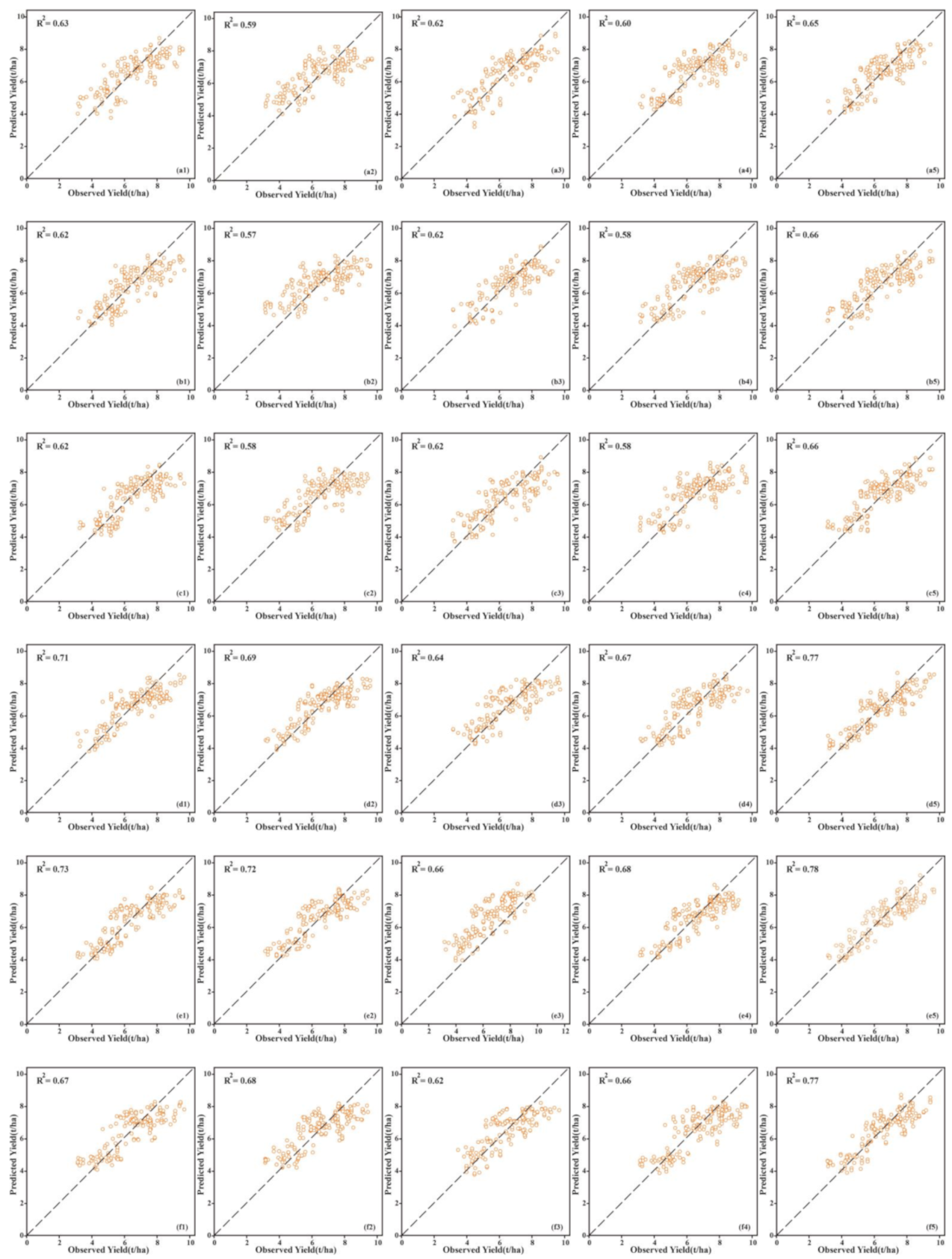
3.3. Comparison and Performance of Feature Selection Methods and Model Accuracy

In order to further explore the high-performance features, a total of 60 features were iteratively added to the machine learning model, starting with the first feature in each order, and updating the model training performance until all of the 60 features were included. The training accuracy was calculated for four base models (SVM, GP, LRR, and RF), obtained under three feature selection methods, for the two wheat growth stages (Figure 5). For the SVM model, the Boruta method performed best in both the flowering and grain-filling stages, followed by PCC and RFE, and the accuracy of the model improved as the number of features increased (Figure 5(a1,2)). For the GP model, the flowering stage was more accurate when using the Boruta method, followed by the PCC and RFE methods, and the grain-filling stage was better with the Boruta method and PCC compared to RFE (Figure 5(b1,2)). For the LRR model, the RFE method performed best at the flowering stage. The Boruta method performed the best at the grain-filling stage and PCC performed the worst (Figure 5(c1,2)). In the RF model, the best accuracy was achieved at the flowering and grain-filling stages when the Boruta method was used to rank the models, with the PCC and RFE methods performing in general agreement at the flowering stage and the results of the RFE method were the worst at the grain-filling stage (Figure 5(d1,2)). The combined results showed that the accuracy of all of the four models (SVM, GP, LRR, and RF) remained stable as the number of features increased after about 25 features. Therefore, this study used the top 25 features for the ensemble model development.

Comparing the R² of the four models constructed for the two growth stages showed that the LRR model had the lowest accuracy, with R² ranging from 0.48 to 0.54 at the flowering stage and 0.48 to 0.63 at the grain-filling stage, and after the input features were stable, the R² values were 0.54 and 0.59, respectively. The R² of the GP model ranged from 0.12 to 0.72 for the flowering stage, and 0.55–0.81 for the grain-filling stage. The RF model had the highest accuracy, with R² ranging from 0.76 to 0.94 at the flowering stage and 0.86–0.95 at the grain-filling stage, and when the input features were stabilized, the R² values were 0.93 and 0.95, respectively.

The five models (four base models and the DLF model) were trained using the full features of the training samples and selected features, and model performance was evaluated on the validation samples. The mean values of the validation accuracy obtained from 200 trials are shown in

Table 4. Test accuracies of the support vector machine (SVM), Gaussian process (GP), linear ridge regression (LRR), random forest (RF), and decision layer fusion (DLF) models in predicting winter wheat yield.

Feature	Model	Flowering				Grain Filling
		R2	RMSE(t/ha)	RPIQ	RPD	R2	RMSE(t/ha)	RPIQ	RPD
Selected features (RFE)	SVM	0.63	1.03	2.40	1.60	0.71	0.90	2.64	1.83
	GP	0.59	1.09	2.25	1.51	0.69	0.94	2.52	1.75
	LRR	0.62	1.03	2.38	1.59	0.64	1.00	2.36	1.64
	RF	0.60	1.05	2.35	1.57	0.67	0.94	2.51	1.74
	DLF	0.65	0.99	2.47	1.65	0.77	0.81	2.94	2.04
Selected features (Boruta)	SVM	0.62	1.03	2.31	1.60	0.73	0.87	2.74	1.90
	GP	0.57	1.11	2.12	1.48	0.72	0.89	2.65	1.84
	LRR	0.62	1.03	2.29	1.59	0.66	0.98	2.42	1.68
	RF	0.58	1.07	2.21	1.54	0.68	0.94	2.53	1.76
	DLF	0.66	0.98	2.40	1.67	0.78	0.79	2.99	2.08
Selected features (PCC)	SVM	0.62	1.03	2.29	1.61	0.67	0.94	2.52	1.74
	GP	0.58	1.11	2.12	1.49	0.68	0.96	2.49	1.71
	LRR	0.62	1.03	2.28	1.60	0.63	1.03	2.32	1.60
	RF	0.58	1.08	2.19	1.54	0.66	0.96	2.47	1.70
	DLF	0.66	0.99	2.39	1.68	0.77	0.82	2.91	2.01
Full features	SVM	0.59	1.05	2.25	1.56	0.68	0.95	2.51	1.73
	GP	0.56	1.10	2.14	1.48	0.67	0.97	2.45	1.69
	LRR	0.58	1.07	2.22	1.53	0.60	1.05	2.26	1.56
	RF	0.57	1.08	2.20	1.52	0.65	0.97	2.44	1.68
	DLF	0.63	1.00	2.36	1.63	0.75	0.84	2.84	1.96

. Among the base models constructed in this study, the validation accuracy of the SVM model constructed using the RFE method with the preferred spectral indices at the flowering stage was the highest (R² = 0.63, RMSE = 1.03 t·ha⁻¹, RPIQ = 2.40, RPD = 1.60), and the validation set accuracy of the SVM model constructed using the Boruta method with the preferred features at the grain-filling stage was the highest (R² = 0.73, RMSE = 0.87 t·ha⁻¹, RPIQ = 2.74, RPD = 1.90). Among the constructed DLF models, the best accuracy of the models constructed using the Boruta and PCC methods with the preferred features at the flowering stage achieved an R² of 0.66, and the highest accuracy of the models constructed using the Boruta method with the preferred features was at the grain-filling stage (R² = 0.78, RMSE = 0.79 t·ha⁻¹, RPIQ = 2.99, RPD = 2.08). Overall, all of the methods gave an R² of 0.56 or higher, indicating the effectiveness of these models in estimating the winter wheat yield. The DLF models outperformed all of the individual models. The R² values for the DLF models constructed using the preferred features were ≥0.65 for the flowering stage, and 0.63 for the DLF models constructed using all features. At the grain-filling stage, the R² values were ≥0.77 for the DLF models constructed using the preferred features, and 0.75 for the DLF models constructed using all of the features at the grain-filling stage. The accuracy of all of the feature selection methods was improved in this study relative to the full feature model, and the RFE method improved the most at the flowering stage. The R² values of the SVM, GP, LRR, RF, and DLF models improved by 0.04, 0.03, 0.04, 0.03, and 0.02, reaching 0.63, 0.59, 0.62, 0.60, and 0.65, respectively, at the flowering stage. The Boruta method improved the most at the grain-filling stage. The R² values for the five models increased by 0.05, 0.05, 0.06, 0.03, and 0.03, reaching 0.73, 0.72, 0.66, 0.68, 0.78, respectively. In addition, the accuracy of the models was higher at the grain-filling stage compared to the flowering stage.

Scatter plots (Figure A1) were used to better show the yield prediction performance of the models and the feature selection methods. In general, all of the models gave good results and performed well with all three of the feature selection methods. In addition, the accuracy of the DLF model varied by growth stage and feature selection method. The performance was stable across all of the feature selection methods at the different growth stages, indicating that it was more adaptable to different feature selection methods. Most of the observed and predicted yields obtained from the DLF model showed good agreement with each other, and it was good at simulating the high and low yields obtained at harvest for the different irrigation treatments.

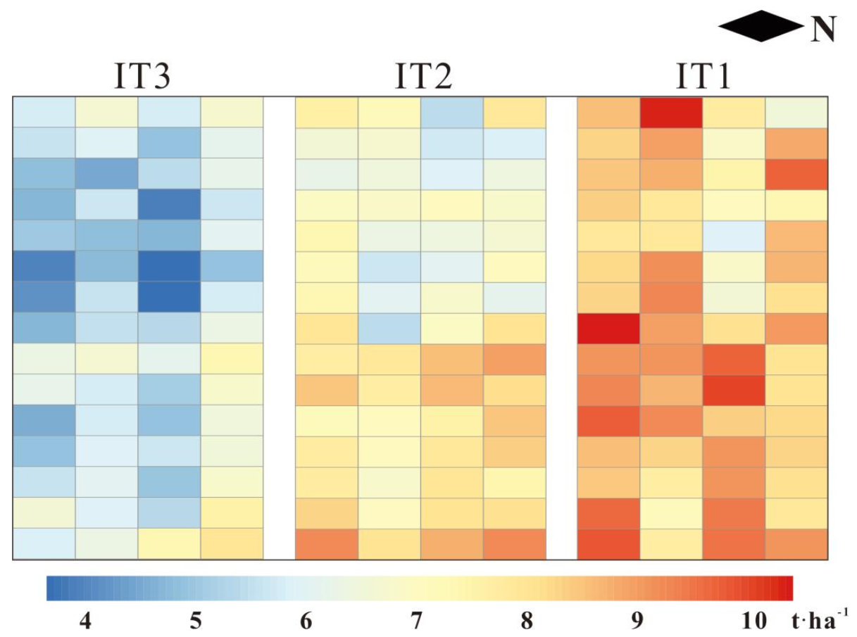
3.4. Yield Distribution

A comparison of all of the models used in this study revealed that the DLF model, constructed using the Boruta method for preferential feature selection at the grain-filling stage, achieved the best accuracy, and it was therefore used to generate a distribution of predicted yields (Figure 6). The results of the t-test analysis between the different irrigation treatments are shown in

Table 5. T-test results for pairwise comparisons of the three irrigation treatments.

Feature	t	p-Value
IT1 VS IT2	7.097	0.000
IT1 VS IT3	16.661	0.000
IT2 VS IT3	9.348	0.000

and indicate that the yield distribution differed significantly between the three treatments, in the order IT1 > IT2 > IT3. Overall, the predicted yield distribution in the IT1 treatment was in the range of 5 to 10 t·ha⁻¹. Based on the observed results, the IT1 treatment had the highest yield of 5 to 9 t·ha⁻¹, followed by the IT2 and IT3 treatments; this is consistent with the yield distribution predicted by the DLF model and demonstrates the feasibility of using a model to estimate yield.

4. Discussion

We selected 60 hyperspectral narrow-band indices for this study, of which approximately 74% were associated with red-rimmed bands. At the flowering stage, more than six indices associated with the red-edge band were in the top 10 after sorting by the RFE, Boruta, and PCC methods. These red-edge spectral indices all provided better prediction performance than other band indices, which agrees with the findings of previous studies [79,80,81]. For example, Xie et al. [82] analyzed the relationship between yield and canopy spectral reflectance of winter wheat at maturity under low-temperature stress and found that the red-edge region was associated with grain yield. However, there was a large variation in the ranking of the different indices, which may be due to the use of different feature selection methods or the different environments to which the vegetation indices apply. Some of the spectral indices performed consistently well among the different feature selection methods at the two wheat growth stages, such as the three spectral indices RVSI, DSWI-4, and ND_[553,682]. The RVSI index, which consists of three bands including the red-edge band, performed well in assessing wheat rust symptoms and constructing rice physiological trait models [83], and was in the top five in the different methodological feature rankings in this study. This could be because it provided more spectral information and was more sensitive to the yield of the different feature selection methods at the different growth stages. The DWSI-4 index, originally a variant of the plant disease-water stress index constructed using simple and normalized ratios, also had good stability and performance in crop disease prediction [84]. The ND_[553,682] index can be used to estimate the chlorophyll content and can minimize the effect of shading and leaf area index size [85,86]. Our study showed that these three spectral indices can be used for yield estimation. MCARI/MTVI2 and TCARI/OSAVI are integrated indices. In previous studies, their performance was better than the individual MCARI, MTVI2, and OSAVI indices, because the integrated indices had richer band information and effectively eliminate the background effects. [87,88]. The Boruta method was second to the RFE method for winter wheat at the flowering stage and performed best at the grain-filling stage, probably due to the difference in the performance between the two methods in the different environments. The Boruta method is a fully correlated feature selection method that aims to select features that are truly correlated with the dependent variable and can be used for prediction, rather than model-specific selection, and can help us to understand the characteristics of the dependent variable more comprehensively and make better and more effective feature selections [24,89]. The RFE method takes into account the correlation between the features, continuously builds models to find the best features, has good generalization ability, and is a suitable method for small sample data sets [90]. The PCC method, which performed the worst in this study, is very commonly used in sensitivity feature selection in the crop science community. It does not require any model training, but does not objectively represent correlations when the correlations between the variables are complex. There is also a risk of multicollinearity between features [91,92]. In this study, the accuracy of the model construction, based on the preferred features under feature selection, was better than that of the model under the full feature condition, which was consistent with the findings of Hsu et al. 2011 [93] and validated the effectiveness and generalizability of the feature selection method.

In this study, four individual machine learning algorithms were used to construct winter wheat yield estimation models based on a subset of spectral indices obtained after feature selection. The RF model had the highest accuracy and performed best when trained using the training set data, but the RF model was not the best performer in the validation set of the model, probably due to the overfitting phenomenon of the RF model in the training set [94]. In the model training set, the LRR models all performed the worst, but in the model validation set the GP models performed the worst at the flowering stage and the LRR models performed the worst at the grain-filling stage. LRR models tend to have a lower R² than the ordinary regression models but can generate a value on covariance problems [95]. The GP models use the full sample for prediction, and as the dimensionality of the data rises, the effectiveness decreases [96]. The SVM models did not perform well in the training set but had the highest accuracy in the validation. SVM is a machine learning method based on the inner product kernel function. The wrong choice of kernel hyperparameters may cause a decrease in the accuracy of the model training set estimation. However, the high accuracy of the SVM model validation set was due to its better robustness, suitability for small sample data regression, and the lack of sensitivity to kernel functions with the ability to avoid dimensional catastrophe problems. [97,98]. We also found that the accuracy of yield estimation models constructed using the four independent machine learning algorithms, SVM, GP, LRR, and RF, at the two developmental stages of winter wheat also differed greatly. Based on the model validation set, the accuracy of each model at the grain-filling stage was higher than that at the flowering stage under the different feature selections. This was due to the dry matter stored in the wheat seeds through carbon assimilation in the winter wheat during grain filling, indicating that this stage contains more spectral information that can be used to predict yield. In addition, the spectral information collected from the winter wheat was increased in order to provide a more comprehensive and accurate reflection of the yield of the winter wheat [2,99].

A DLF (decision-level fusion) model was developed based on the individual machine learning models used in this study. The results showed that the DLF model performed significantly better than each of the other models when all of the features or the selected features were used. When using the selected features, the DLF model performed best at the flowering and grain-filling stages, and the model accuracy was better than that of the individual models. In addition, using selected features obtained under the different feature selection methods, the DLF model produced R² values of >0.65 at the flowering stage and >0.77 at the grain-filling stage. Overall, the DLF model gave more satisfactory and better results than the individual models. This was the same conclusion reached in a previous study [33] where the DLF model was able to minimize the individual model bias and improve the accuracy of the inverse model. Taken together, the above description suggests that adequacy and diversity are two important principles in the selection of base models in the decision-level fusion process [100]. This requires that the different base learners should all have a good predictive performance and be able to minimize inter-model dependencies and act as complementary information [101,102]. This prerequisite requirement is justified by the fact that the DLF methods fuse the prediction results of different independent machine learners so that the final fusion results are all influenced by each base model [103]. Furthermore, fusion of models with similar high performance will yield limited prediction results [104]. Based on the requirements of DLF and the limitation problem, this study used the SVM, GP, LRR, and RF machine learning algorithms with completely different training mechanisms to construct the yield estimation models and improved the model performance through parameter optimization, and the experimental results provided further evidence of the effectiveness of the underlying models.

This study used the acquired hyperspectral image time series to predict the yield of winter wheat, and the yield prediction model constructed for the grain-filling period had a high accuracy rate. The use of hyperspectral data to construct yield estimation models has been widely used in previous yield estimation studies, and all have achieved high model accuracy, consistent with the findings of this paper [105,106]. For example, Chandel et al. (2019) [107] used hyperspectral indices to construct a yield prediction regression model and found that the yield of irrigated wheat was estimated with an accuracy of 96%. However, relying on hyperspectral data alone for yield estimation still has some limitations. In future research, we intend to integrate UAV RGB and multispectral image data into yield estimation models as well, in order to broaden the application area of yield estimation. In addition, we will also consider examining the effects of biotic (weeds, pests, and diseases) and abiotic (nutrients, temperature, and salinity) stresses based on UAV imagery and ground data. Finally, additional feature selection methods and integrated learning methods will be considered for yield estimation in order to further improve the prediction accuracy. Therefore, in the future, we will also analyze the impact of diseases, insects, and fertility on wheat yield.

5. Conclusions

In winter wheat production, real-time insight into yield conditions prior to harvesting can help to optimize crop management and guide the field practices. In this study, we developed a DLF-based machine learning model for winter wheat yield prediction using UAV-based hyperspectral imagery. The narrow-band hyperspectral indices were extracted, and the most important indices were selected for model development using each of the three feature selection methods. The results showed that the RFE-based method for feature selection at the flowering stage had a higher accuracy, the Boruta-based method for feature selection at the grain-filling stage had a higher accuracy, and the DLF model outperformed the base models and achieved the highest accuracy when using the preferred features. This study demonstrates the effectiveness of using hyperspectral images to build a model for yield estimation in winter wheat.

References

1. Nausheen, M.; Shirazi, S.A.; Stringer, L.C.; Sohail, M. Using UAV imagery to measure plant and water stress in winter wheat fields of drylands, south Punjab, Pakistan. Pak. J. Agric. Sci. 2021, 58, 1041–1050. [Google Scholar]
2. Fei, S.; Hassan, M.; He, Z.; Chen, Z.; Shu, M.; Wang, J.; Li, C.; Xiao, Y. Assessment of Ensemble Learning to Predict Wheat Grain Yield Based on UAV-Multispectral Reflectance. Remote Sens. 2021, 13, 2338. [Google Scholar] [CrossRef]
3. Yue, J.; Zhou, C.; Guo, W.; Feng, H.; Xu, K. Estimation of winter-wheat above-ground biomass using the wavelet analysis of unmanned aerial vehicle-based digital images and hyperspectral crop canopy images. Int. J. Remote Sens. 2021, 42, 1602–1622. [Google Scholar] [CrossRef]
4. Galan, R.J.; Bernal-Vasquez, A.; Jebsen, C.; Piepho, H.; Thorwarth, P.; Steffan, P.; Gordillo, A.; Miedaner, T. Integration of genotypic, hyperspectral, and phenotypic data to improve biomass yield prediction in hybrid rye. Theor. Appl. Genet. 2020, 133, 3001–3015. [Google Scholar] [CrossRef]
5. Yue, J.; Feng, H.; Li, Z.; Zhou, C.; Xu, K. Mapping winter-wheat biomass and grain yield based on a crop model and UAV remote sensing. Int. J. Remote Sens. 2021, 42, 1577–1601. [Google Scholar] [CrossRef]
6. Zhou, X.; Kono, Y.; Win, A.; Matsui, T.; Tanaka, T.S.T. Predicting within-field variability in grain yield and protein content of winter wheat using UAV-based multispectral imagery and machine learning approaches. Plant. Prod. Sci. 2020, 24, 137–151. [Google Scholar] [CrossRef]
7. Li, B.; Xu, X.; Zhang, L.; Han, J.; Bian, C.; Li, G.; Liu, J.; Jin, L. Above-ground biomass estimation and yield prediction in potato by using UAV-based RGB and hyperspectral imaging. ISPRS J. Photogramm. 2020, 162, 161–172. [Google Scholar] [CrossRef]
8. Wheeler, T.; von Braun, J. Climate Change Impacts on Global Food Security. Science 2013, 341, 508–513. [Google Scholar] [CrossRef]
9. Ma, B.L.; Dwyer, L.M.; Costa, C.; Cober, E.R.; Morrison, M.J. Early prediction of soybean yield from canopy reflectance measurements. Agron. J. 2001, 93, 1227–1234. [Google Scholar] [CrossRef] [Green Version]
10. Elsayed, S.; El-Hendawy, S.; Khadr, M.; Elsherbiny, O.; Al-Suhaibani, N.; Alotaibi, M.; Tahir, M.U.; Darwish, W. Combining Thermal and RGB Imaging Indices with Multivariate and Data-Driven Modeling to Estimate the Growth, Water Status, and Yield of Potato under Different Drip Irrigation Regimes. Remote Sens. 2021, 13, 1679. [Google Scholar] [CrossRef]
11. Fernandez-Manso, A.; Fernandez-Manso, O.; Quintano, C. SENTINEL-2A red-edge spectral indices suitability for discriminating burn severity. Int. J. Appl. Earth Obs. 2016, 50, 170–175. [Google Scholar] [CrossRef]
12. Jiao, C.; Zheng, G.; Xie, X.; Cui, X.; Shang, G. Prediction of Soil Organic Matter Using Visible-Short Near-Infrared Imaging Spectroscopy. Spectrosc. Spect. Anal. 2020, 40, 3277–3281. [Google Scholar]
13. Han, Y.; Liu, H.; Zhang, X.; Yu, Z.; Meng, X.; Kong, F.; Song, S.; Han, J. Prediction Model of Rice Panicles Blast Disease Degree Based on Canopy Hyperspectral Reflectance. Spectrosc. Spect. Anal. 2021, 41, 1220–1226. [Google Scholar]
14. Zhang, Y.; Tian, Y.; Sun, W.; Mu, X.; Gao, P.; Zhao, G. Effects of Different Fertilization Conditions on Canopy Spectral Characteristics of Winter Wheat Based on Hyperspectral Technique. Spectrosc. Spect. Anal. 2020, 40, 535–542. [Google Scholar]
15. Liu, Y.; Sun, Q.; Feng, H.; Yang, F. Estimation of Above-Ground Biomass of Potato Based on Wavelet Analysis. Spectrosc. Spect. Anal. 2021, 41, 1205–1212. [Google Scholar]
16. Galan, R.J.; Bernal-Vasquez, A.; Jebsen, C.; Piepho, H.; Thorwarth, P.; Steffan, P.; Gordillo, A.; Miedaner, T. Early prediction of biomass in hybrid rye based on hyperspectral data surpasses genomic predictability in less-related breeding material. Theor. Appl. Genet. 2021, 134, 1409–1422. [Google Scholar] [CrossRef]
17. Guo, W.; Qiao, H.; Zhao, H.; Zhang, J.; Pei, P.; Liu, Z. Cotton Aphid Damage Monitoring Using UAV Hyperspectral Data Based on Derivative of Ratio Spectroscopy. Spectrosc. Spect. Anal. 2021, 41, 1543–1550. [Google Scholar]
18. Liu, Y.; Feng, H.; Huang, J.; Yang, F.; Wu, Z.; Sun, Q.; Yang, G. Estimation of Potato Above-Ground Biomass Based on Hyperspectral Characteristic Parameters of UAV and Plant Height. Spectrosc. Spect. Anal. 2021, 41, 903–911. [Google Scholar]
19. Wang, L.; Chen, S.; Li, D.; Wang, C.; Jiang, H.; Zheng, Q.; Peng, Z. Estimation of Paddy Rice Nitrogen Content and Accumulation Both at Leaf and Plant Levels from UAV Hyperspectral Imagery. Remote Sens. 2021, 13, 2956. [Google Scholar] [CrossRef]
20. Nidamanuri, R.R.; Zbell, B. Use of field reflectance data for crop mapping using airborne hyperspectral image. ISPRS J. Photogramm. Remote Sens. 2011, 66, 683–691. [Google Scholar] [CrossRef]
21. Yang, C.; Everitt, J.H.; Fernandez, C.J. Comparison of airborne multispectral and hyperspectral imagery for mapping cotton root rot. Biosyst. Eng. 2010, 107, 131–139. [Google Scholar] [CrossRef]
22. Almugren, N.; Alshamlan, H. A Survey on Hybrid Feature Selection Methods in Microarray Gene Expression Data for Cancer Classification. IEEE Access 2019, 7, 78533–78548. [Google Scholar] [CrossRef]
23. Jebli, I.; Belouadha, F.; Kabbaj, M.I.; Tilioua, A. Prediction of solar energy guided by Pearson correlation using machine learning. Energy 2021, 224, 124109. [Google Scholar] [CrossRef]
24. Miron, B.K.; Witold, R.R. Feature Selection with the Boruta Package. J. Stat. Softw. 2010, 36, 11. [Google Scholar]
25. Zhao, J.; Karimzadeh, M.; Masjedi, A.; Wang, T.; Ebert, D.S. FeatureExplorer: Interactive Feature Selection and Exploration of Regression Models for Hyperspectral Images. In Proceedings of the 2019 IEEE Visualization Conference (VIS), Vancouver, BC, Canada, 20–25 October 2019; pp. 161–165. [Google Scholar]
26. Feng, L.; Zhang, Z.; Ma, Y.; Du, Q.; Williams, P.; Drewry, J.; Luck, B. Alfalfa Yield Prediction Using UAV-Based Hyperspectral Imagery and Ensemble Learning. Remote Sens. 2020, 12, 2028. [Google Scholar] [CrossRef]
27. Pal, M. Ensemble Learning with Decision Tree for Remote Sensing Classification. Pro. World Acad. Sci. Eng. Technol. 2007, 26, 735–737. [Google Scholar]
28. Jiang, H.; Tao, C.; Dong, Y.; Xiong, R. Robust low-rank multiple kernel learning with compound regularization. Eur. J. Oper. Res. 2021, 295, 634–647. [Google Scholar] [CrossRef]
29. Peterson, K.T.; Sagan, V.; Sidike, P.; Hasenmueller, E.A.; Sloan, J.J.; Knouft, J.H. Machine Learning-Based Ensemble Prediction of Water-Quality Variables Using Feature-Level and Decision-Level Fusion with Proximal Remote Sensing. Photogramm. Eng. Rem. S. 2019, 85, 269–280. [Google Scholar] [CrossRef]
30. Liang, L.; Yang, M.; Deng, K.; Zhang, L.; Lin, H.; Liu, Z. A new hyperspectral index for the estimation of nitrogen contents of wheat canopy. Acta Ecol. Sin. 2011, 31, 6594–6605. [Google Scholar]
31. Ye, X.; Sakai, K.; He, Y. Development of Citrus Yield Prediction Model Based on Airborne Hyperspectral Imaging. Spectrosc. Spect. Anal. 2010, 30, 1295–1300. [Google Scholar]
32. Xu, B.; Wen, G.; Su, Y.; Zhang, Z.; Chen, F.; Sun, Y. Application of multi-level information fusion for wear particle recognition of ferrographic images. Opt. Precis. Eng. 2018, 26, 1551–1560. [Google Scholar]
33. Tewary, S.; Mukhopadhyay, S. HER2 Molecular Marker Scoring Using Transfer Learning and Decision Level Fusion. J. Digit. Imaging 2021, 34, 667. [Google Scholar] [CrossRef]
34. Teng, S.; Chen, G.; Liu, Z.; Cheng, L.; Sun, X. Multi-Sensor and Decision-Level Fusion-Based Structural Damage Detection Using a One-Dimensional Convolutional Neural Network. Sensors 2021, 21, 3950. [Google Scholar] [CrossRef]
35. Zhao, P.; Li, Z.Y.; Wang, C.K. Wood Species Recognition Based on Visible and Near-Infrared Spectral Analysis Using Fuzzy Reasoning and Decision-Level Fusion. J. Spectrosc. 2021, 2021, 1–16. [Google Scholar] [CrossRef]
36. Attard, L.; Debono, C.J.; Valentino, G.; Di Castro, M. Vision-Based Tunnel Lining Health Monitoring via Bi-Temporal Image Comparison and Decision-Level Fusion of Change Maps. Sensors 2021, 21, 4040. [Google Scholar] [CrossRef]
37. Yu, R.; Luo, Y.; Zhou, Q.; Zhang, X.; Wu, D.; Ren, L. A machine learning algorithm to detect pine wilt disease using UAV-based hyperspectral imagery and LiDAR data at the tree level. Int. J. Appl. Earth Obs. 2021, 101, 102363. [Google Scholar] [CrossRef]
38. Ma, H.; Huang, W.; Dong, Y.; Liu, L.; Guo, A. Using UAV-Based Hyperspectral Imagery to Detect Winter Wheat Fusarium Head Blight. Remote Sens. 2021, 13, 3024. [Google Scholar] [CrossRef]
39. Ashourloo, D.; Mobasheri, M.R.; Huete, A. Evaluating the Effect of Different Wheat Rust Disease Symptoms on Vegetation Indices Using Hyperspectral Measurements. Remote Sens. 2014, 6, 5107–5123. [Google Scholar] [CrossRef] [Green Version]
40. Singh, K.D.; Duddu, H.S.N.; Vail, S.; Parkin, I.; Shirtliffe, S.J. UAV-Based Hyperspectral Imaging Technique to Estimate Canola (Brassica napus L.) Seedpods Maturity. Can. J. Remote Sens. 2021, 47, 33–47. [Google Scholar] [CrossRef]
41. Zarco-Tejada, P.J.; Pushnik, J.C.; Dobrowski, S.; Ustin, S.L. Steady-state chlorophyll a fluorescence detection from canopy derivative reflectance and double-peak red-edge effects. Remote Sens. Environ. 2003, 84, 283–294. [Google Scholar] [CrossRef]
42. Vergara-Diaz, O.; Zaman-Allah, M.A.; Masuka, B.; Hornero, A.; Zarco-Tejada, P.; Prasanna, B.M.; Cairns, J.E.; Araus, J.L. A Novel Remote Sensing Approach for Prediction of Maize Yield Under Different Conditions of Nitrogen Fertilization. Front. Plant. Sci. 2016, 7, 666. [Google Scholar] [CrossRef] [Green Version]
43. Datt, B. A new reflectance index for remote sensing of chlorophyll content in higher plants: Tests using Eucalyptus leaves. J. Plant. Physiol. 1999, 154, 30–36. [Google Scholar] [CrossRef]
44. le Maire, G.; Francois, C.; Dufrene, E. Towards universal broad leaf chlorophyll indices using PROSPECT simulated database and hyperspectral reflectance measurements. Remote Sens. Environ. 2004, 89, 1–28. [Google Scholar] [CrossRef]
45. Main, R.; Cho, M.A.; Mathieu, R.; O’Kennedy, M.M.; Ramoelo, A.; Koch, S. An investigation into robust spectral indices for leaf chlorophyll estimation. ISPRS J. Photogramm. 2011, 66, 751–761. [Google Scholar] [CrossRef]
46. Hunt, E.R., Jr.; Daughtry, C.S.T.; Eitel, J.U.H.; Long, D.S. Remote Sensing Leaf Chlorophyll Content Using a Visible Band Index. Agron. J. 2011, 103, 1090–1099. [Google Scholar] [CrossRef] [Green Version]
47. Pu, R.; Gong, P.; Yu, Q. Comparative analysis of EO-1 ALI and Hyperion, and Landsat ETM+ data for mapping forest crown closure and leaf area index. Sensors 2008, 8, 3744–3766. [Google Scholar] [CrossRef] [Green Version]
48. Herrmann, I.; Karnieli, A.; Bonfil, D.J.; Cohen, Y.; Alchanatis, V. SWIR-based spectral indices for assessing nitrogen content in potato fields. Int. J. Remote Sens. 2010, 31, 5127–5143. [Google Scholar] [CrossRef]
49. Jurgens, C. The modified normalized difference vegetation index (mNDVI)—a new index to determine frost damages in agriculture based on Landsat TM data. Int. J. Remote Sens. 1997, 18, 3583–3594. [Google Scholar] [CrossRef]
50. Dash, J.; Curran, P.J. The MERIS terrestrial chlorophyll index. Int. J. Remote Sens. 2004, 25, 5403–5413. [Google Scholar] [CrossRef]
51. Haboudane, D.; Miller, J.R.; Pattey, E.; Zarco-Tejada, P.J.; Strachan, I.B. Hyperspectral vegetation indices and novel algorithms for predicting green LAI of crop canopies: Modeling and validation in the context of precision agriculture. Remote Sens. Environ. 2004, 90, 337–352. [Google Scholar] [CrossRef]
52. le Maire, G.; Francois, C.; Soudani, K.; Berveiller, D.; Pontailler, J.; Breda, N.; Genet, H.; Davi, H.; Dufrene, E. Calibration and validation of hyperspectral indices for the estimation of broadleaved forest leaf chlorophyll content, leaf mass per area, leaf area index and leaf canopy biomass. Remote Sens. Environ. 2008, 112, 3846–3864. [Google Scholar] [CrossRef]
53. Richardson, A.D.; Duigan, S.P.; Berlyn, G.P. An evaluation of noninvasive methods to estimate foliar chlorophyll content. New Phytol. 2002, 153, 185–194. [Google Scholar] [CrossRef] [Green Version]
54. Metternicht, G. Vegetation indices derived from high-resolution airborne videography for precision crop management. Int. J. Remote Sens. 2003, 24, 2855–2877. [Google Scholar] [CrossRef]
55. Aparicio, N.; Villegas, D.; Royo, C.; Casadesus, J.; Araus, J.L. Effect of sensor view angle on the assessment of agronomic traits by ground level hyper-spectral reflectance measurements in durum wheat under contrasting Mediterranean conditions. Int. J. Remote Sens. 2004, 25, 1131–1152. [Google Scholar] [CrossRef]
56. Royo, C.; Aparicio, N.; Villegas, D.; Casadesus, J.; Monneveux, P.; Araus, J.L. Usefulness of spectral reflectance indices as durum wheat yield predictors under contrasting Mediterranean conditions. Int. J. Remote Sens. 2003, 24, 4403–4419. [Google Scholar] [CrossRef]
57. Wu, C.; Niu, Z.; Tang, Q.; Huang, W. Estimating chlorophyll content from hyperspectral vegetation indices: Modeling and validation. Agric. For. Meteorol. 2008, 148, 1230–1241. [Google Scholar] [CrossRef]
58. Rao, N.R.; Garg, P.K.; Ghosh, S.K.; Dadhwal, V.K. Estimation of leaf total chlorophyll and nitrogen concentrations using hyperspectral satellite imagery. J. Agric. Sci. 2008, 146, 65–75. [Google Scholar]
59. Ceccato, P.; Gobron, N.; Flasse, S.; Pinty, B.; Tarantola, S. Designing a spectral index to estimate vegetation water content from remote sensing data: Part 1—Theoretical approach. Remote Sens. Environ. 2002, 82, 188–197. [Google Scholar] [CrossRef]
60. Penuelas, J.; Gamon, J.A.; Fredeen, A.L.; Merino, J.; Field, C.B. Reflectance indices associated with physiological changes in nitrogen- and water-limited sunflower leaves. Remote Sens. Environ. 1994, 48, 135–146. [Google Scholar] [CrossRef]
61. Blackburn, G.A. Spectral indices for estimating photosynthetic pigment concentrations: A test using senescent tree leaves. Int. J. Remote Sens. 1998, 19, 657–675. [Google Scholar] [CrossRef]
62. Sims, D.A.; Gamon, J.A. Relationships between leaf pigment content and spectral reflectance across a wide range of species, leaf structures and developmental stages. Remote Sens. Environ. 2002, 81, 337–354. [Google Scholar] [CrossRef]
63. Galvao, L.S.; Formaggio, A.R.; Tisot, D.A. Discrimination of sugarcane varieties in southeastern Brazil with EO-1 hyperion data. Remote Sens. Environ. 2005, 94, 523–534. [Google Scholar] [CrossRef]
64. Underwood, E.; Ustin, S.; DiPietro, D. Mapping nonnative plants using hyperspectral imagery. Remote Sens. Environ. 2003, 86, 150–161. [Google Scholar] [CrossRef]
65. Clevers, J.; De Jong, S.M.; Epema, G.F.; Van der Meer, F.D.; Bakker, W.H.; Skidmore, A.K.; Scholte, K.H. Derivation of the red edge index using the MERIS standard band setting. Int. J. Remote Sens. 2002, 23, 3169–3184. [Google Scholar] [CrossRef] [Green Version]
66. Azadbakht, M.; Ashourloo, D.; Aghighi, H.; Radiom, S.; Alimohammadi, A. Wheat leaf rust detection at canopy scale under different LAI levels using machine learning techniques. Comput. Electron. Agric. 2019, 156, 119–128. [Google Scholar] [CrossRef]
67. Wu, J.; Wang, D.; Bauer, M.E. Assessing broadband vegetation indices and QuickBird data in estimating leaf area index of corn and potato canopies. Field Crop. Res. 2007, 102, 33–42. [Google Scholar] [CrossRef]
68. Lichtenthaler, H.K. Vegetation stress: An introduction to the stress concept in plants. J. Plant. Physiol. 1996, 148, 4–14. [Google Scholar] [CrossRef]
69. Gitelson, A.A.; Merzlyak, M.N. Remote estimation of chlorophyll content in higher plant leaves. Int. J. Remote Sens. 1997, 18, 2691–2697. [Google Scholar] [CrossRef]
70. Broge, N.H.; Leblanc, E. Comparing prediction power and stability of broadband and hyperspectral vegetation indices for estimation of green leaf area index and canopy chlorophyll density. Remote Sens. Environ. 2001, 76, 156–172. [Google Scholar] [CrossRef]
71. Guyon, I.; Weston, J.; Barnhill, S.; Vapnik, V. Gene selection for cancer classification using support vector machines. Mach. Learn. 2002, 46, 389–422. [Google Scholar] [CrossRef]
72. Ramendra, P.; Ravinesh, C.D.; Yan, L.; Tek, M. Weekly soil moisture forecasting with multivariate sequential, ensemble empirical mode decomposition and Boruta-random forest hybridizer algorithm approach. Catena 2019, 177, 149–166. [Google Scholar]
73. Gholami, H.; Mohammadifar, A.; Golzari, S.; Kaskaoutis, D.G.; Collins, A.L. Using the Boruta algorithm and deep learning models for mapping land susceptibility to atmospheric dust emissions in Iran. Aeolian Res. 2021, 50, 100682. [Google Scholar] [CrossRef]
74. Wang, L.; Zhou, X.; Zhu, X.; Dong, Z.; Guo, W. Estimation of biomass in wheat using random forest regression algorithm and remote sensing data. Crop. J. 2016, 4, 212–219. [Google Scholar] [CrossRef] [Green Version]
75. Zhai, Y.; Cui, L.; Zhou, X.; Gao, Y.; Fei, T.; Gao, W. Estimation of nitrogen, phosphorus, and potassium contents in the leaves of different plants using laboratory-based visible and near-infrared reflectance spectroscopy: Comparison of partial least-square regression and support vector machine regression methods. Int. J. Remote Sens. 2013, 34, 2502–2518. [Google Scholar]
76. Chlingaryan, A.; Sukkarieh, S.; Whelan, B. Machine learning approaches for crop yield prediction and nitrogen status estimation in precision agriculture: A review. Comput. Electron. Agric. 2018, 151, 61–69. [Google Scholar] [CrossRef]
77. Chen, C.C.; Schwender, H.; Keith, J.; Nunkesser, R.; Mengersen, K.; Macrossan, P. Methods for Identifying SNP Interactions: A Review on Variations of Logic Regression, Random Forest and Bayesian Logistic Regression. IEEE ACM Trans. Comput. Bi. 2011, 8, 1580–1591. [Google Scholar] [CrossRef]
78. Wang, J.; Shi, T.; Yu, D.; Teng, D.; Ge, X.; Zhang, Z.; Yang, X.; Wang, H.; Wu, G. Ensemble machine-learning-based framework for estimating total nitrogen concentration in water using drone-borne hyperspectral imagery of emergent plants: A case study in an arid oasis, NW China. Environ. Pollut. 2020, 266, 115412. [Google Scholar] [CrossRef]
79. Xianxian, G.; Mao, W.; Mingming, J.; Wenqing, W. Estimating mangrove leaf area index based on red-edge vegetation indices: A comparison among UAV, WorldView-2 and Sentinel-2 imagery. Int. J. Appl. Earth Obs. 2021, 103, 102493. [Google Scholar]
80. Yu, Z.; Jian-wen, W.; Li-ping, C.; Yuan-yuan, F.U.; Hong-chun, Z.; Hai-kuan, F.; Xin-gang, X.U.; Zhen-hai, L.I. An entirely new approach based on remote sensing data to calculate the nitrogen nutrition index of winter wheat. J. Integr. Agric. 2021, 20, 2535–2551. [Google Scholar]
81. Zhu, Y.; Liu, K.; Liu, L.; Myint, S.W.; Wang, S.; Liu, H.; He, Z. Exploring the Potential of WorldView-2 Red-Edge Band-Based Vegetation Indices for Estimation of Mangrove Leaf Area Index with Machine Learning Algorithms. Remote Sens. 2017, 9, 1060. [Google Scholar] [CrossRef] [Green Version]
82. Xie, Y.; Wang, C.; Yang, W.; Feng, M.; Qiao, X.; Song, J. Canopy hyperspectral characteristics and yield estimation of winter wheat (Triticum aestivum) under low temperature injury. Sci. Rep. 2020, 10, 109–119. [Google Scholar] [CrossRef] [PubMed] [Green Version]
83. Li, G.; Xiang-Nan, L.; Cheng-Qi, C. Research on hyperspectral information parameters of chlorophyll content of rice leaf in Cd-polluted soil environment. Guang Pu Xue Yu Guang Pu Fen Xi 2009, 29, 2713–2716. [Google Scholar]
84. Apan, A.; Held, A.; Phinn, S.; Markley, J. Detecting sugarcane ‘orange rust’ disease using EO-1 Hyperion hyperspectral imagery. Int. J. Remote Sens. 2004, 25, 489–498. [Google Scholar] [CrossRef] [Green Version]
85. Padalia, H.; Sinha, S.K.; Bhave, V.; Trivedi, N.K.; Kumar, A.S. Estimating canopy LAI and chlorophyll of tropical forest plantation (North India) using Sentinel-2 data. Adv. Space Res. 2020, 65, 458–469. [Google Scholar] [CrossRef]
86. Cui, B.; Zhao, Q.; Huang, W.; Song, X.; Ye, H.; Zhou, X. Leaf chlorophyll content retrieval of wheat by simulated RapidEye, Sentinel-2 and EnMAP data. J. Integr. Agric. 2019, 18, 1230–1245. [Google Scholar] [CrossRef]
87. Lin, W.; Huang, J.; Hu, X.; Zhao, M. Crop Yield Forecast Based On Modis Temperature-Vegetation Angel Index. J. Infrared Millim. W. 2010, 29, 476–480. [Google Scholar]
88. Cao, S.; Liu, X.; Liu, M.; Cao, S.; Yao, S. Estimation of Leaf Area Index by Normalized Composite Vegetation Index Fusing the Spectral Feature of Canopy Water Content. Spectrosc. Spect. Anal. 2011, 31, 478–482. [Google Scholar]
89. Kursa, M.B.; Jankowski, A.; Rudnicki, W.R. Boruta—A System for Feature Selection. Fund. Inform. 2010, 101, 271–285. [Google Scholar] [CrossRef]
90. Paul, J.; Ambrosio, R.D.; Dupont, P. Kernel methods for heterogeneous feature selection. Neurocomputing 2015, 169, 187–195. [Google Scholar] [CrossRef] [Green Version]
91. Salleh, F.H.M.; Arif, S.M.; Zainudin, S.; Firdaus-Raih, M. Reconstructing gene regulatory networks from knock-out data using Gaussian Noise Model and Pearson Correlation Coefficient. Comput. Biol. Chem. 2015, 59, 3–14. [Google Scholar] [CrossRef]
92. Jain, D.K.A.; Shetty, N.; Naveen Kumar, L.; Sundaresh, D.C. Assessment of Usefulness of Anthropometric Data for Predicting the Scaphoid and the Screw Length: A New Technique. J. Hand Surg. Asian-Pac. Volume 2017, 22, 435–440. [Google Scholar] [CrossRef]
93. Hsu, H.; Hsieh, C.; Lu, M. Hybrid feature selection by combining filters and wrappers. Expert Syst. Appl. 2011, 38, 8144–8150. [Google Scholar] [CrossRef]
94. Ge, X.; Ding, J.; Wang, J.; Sun, H.; Zhu, Z. A New Method for Predicting Soil Moisture Based on UAV Hyperspectral Image. Spectrosc. Spect. Anal. 2020, 40, 602–609. [Google Scholar]
95. Joris, T.; Jaak, S.; Karl, M.; Yves, M. Two-level preconditioning for Ridge Regression. Numer. Linear Algebr. 2021, 28, 2371. [Google Scholar]
96. Yuanyuan, L.; Qianqian, Z.; Won, Y.S. Gaussian process regression-based learning rate optimization in convolutional neural networks for medical images classification. Expert Syst. Appl. 2021, 184, 115357. [Google Scholar]
97. Elbeltagi, A.; Azad, N.; Arshad, A.; Mohammed, S.; Mokhtar, A.; Pande, C.; Etedali, H.R.; Bhat, S.A.; Islam, A.R.M.T.; Deng, J. Applications of Gaussian process regression for predicting blue water footprint: Case study in Ad Daqahliyah, Egypt. Agric. Water Manag. 2021, 255, 107052. [Google Scholar] [CrossRef]
98. Shafaei, M.; Kisi, O. Predicting river daily flow using wavelet-artificial neural networks based on regression analyses in comparison with artificial neural networks and support vector machine models. Neural Comput. Appl. 2017, 28, 15–28. [Google Scholar] [CrossRef]
99. Jurečka, F.; Fischer, M.; Hlavinka, P.; Balek, J.; Semerádová, D.; Bláhová, M.; Anderson, M.C.; Hain, C.; Žalud, Z.; Trnka, M. Potential of water balance and remote sensing-based evapotranspiration models to predict yields of spring barley and winter wheat in the Czech Republic. Agric. Water Manag. 2021, 256, 107064. [Google Scholar] [CrossRef]
100. Bhavya, D.N.; Chethan, H.K. Feature and Decision Level Fusion in Children Multimodal Biometrics. Int. J. Recent Technol. Eng. (IJRTE). 2020, 8, 2522–2527. [Google Scholar]
101. Fu, H.; Cui, G.; Li, X.; She, W.; Cui, D.; Zhao, L.; Su, X.; Wang, J.; Cao, X.; Liu, J.; et al. Estimation of ramie yield based on UAV (Unmanned Aerial Vehicle) remote sensing images. Acta Agron. Sin. 2020, 46, 1448–1455. [Google Scholar]
102. Yuri, S.; Robert, D.; Peter, T. Integrating satellite imagery and environmental data to predict field-level cane and sugar yields in Australia using machine learning. Field Crop. Res. 2021, 260, 107984. [Google Scholar]
103. Shen, B.; Liu, Y.; Fu, J. An Integrated Model for Robust Multisensor Data Fusion. Sensors 2014, 14, 19669–19686. [Google Scholar] [CrossRef] [Green Version]
104. Verrelst, J.; Muñoz, J.; Alonso, L.; Delegido, J.; Rivera, J.P.; Camps-Valls, G.; Moreno, J. Machine learning regression algorithms for biophysical parameter retrieval: Opportunities for Sentinel-2 and-3. Remote Sens. Environ. 2012, 118, 127–139. [Google Scholar] [CrossRef]
105. Garriga, M.; Romero-Bravo, S.; Estrada, F.; Mendez-Espinoza, A.M.; Gonzalez-Martinez, L.; Matus, I.A.; Castillo, D.; Lobos, G.A.; Del Pozo, A. Estimating carbon isotope discrimination and grain yield of bread wheat grown under water-limited and full irrigation conditions by hyperspectral canopy reflectance and multilinear regression analysis. Int. J. Remote Sens. 2021, 42, 2848–2871. [Google Scholar] [CrossRef]
106. Zhang, X.; Zhao, J.; Yang, G.; Liu, J.; Cao, J.; Li, C.; Zhao, X.; Gai, J. Establishment of Plot-Yield Prediction Models in Soybean Breeding Programs Using UAV-Based Hyperspectral Remote Sensing. Remote Sens. 2019, 11, 2752. [Google Scholar] [CrossRef] [Green Version]
107. Chandel, N.S.; Tiwari, P.S.; Singh, K.P.; Jat, D.; Gaikwad, B.B.; Tripathi, H.; Golhani, K. Yield prediction in wheat (Triticum aestivum L.) using spectral reflectance indices. Curr. Sci. 2019, 116, 272–278. [Google Scholar] [CrossRef]
Figure 1. Meteorological conditions during the wheat growth period from November to May: (a) total monthly rainfall, (b) average monthly temperature, (c) average monthly humidity, and (d) average monthly sunshine hours.
Agronomy 12 00202 g001
Figure 2. Distribution of test sites and test plots. IT1: high irrigation; IT2: moderate irrigation; IT3: low irrigation.
Agronomy 12 00202 g002
Figure 3. Workflow of a DLF (decision-level fusion) model for grain yield prediction; the model included SVM (support vector machine), GP (Gaussian process), LRR (linear ridge regression), and RF (random forest). The “e” is the model prediction.
Agronomy 12 00202 g003
Figure 4. Five-fold cross-validation internal and external cross-validation strategies.
Agronomy 12 00202 g004
Figure 5. The relationships between model training accuracy and number of features. (a1,a2), SVM model at the flowering and grain-filling stages, respectively; (b1,b2), GP model at flowering and grain-filling stages, respectively; (c1,c2) LRR model at flowering and grain-filling stages, respectively; (d1,d2) RF model at flowering and grain-filling stages, respectively.
Agronomy 12 00202 g005
Figure 6. Yield distribution chart for the three irrigation treatments. The color scale from blue to red indicates the increasing grain yield from 4 to 10 t ha−1.
Agronomy 12 00202 g006