Daily Prediction and Multi-Step Forward Forecasting of Reference Evapotranspiration Using LSTM and Bi-LSTM Models

Abstract

Precise forecasting of reference evapotranspiration (ET₀) is one of the critical initial steps in determining crop water requirements, which contributes to the reliable management and long-term planning of the world’s scarce water sources. This study provides daily prediction and multi-step forward forecasting of ET₀ utilizing a long short-term memory network (LSTM) and a bi-directional LSTM (Bi-LSTM) model. For daily predictions, the LSTM model’s accuracy was compared to that of other artificial intelligence-based models commonly used in ET0 forecasting, including support vector regression (SVR), M5 model tree (M5Tree), multivariate adaptive regression spline (MARS), probabilistic linear regression (PLR), adaptive neuro-fuzzy inference system (ANFIS), and Gaussian process regression (GPR). The LSTM model outperformed the other models in a comparison based on Shannon’s entropy-based decision theory, while the M5 tree and PLR models proved to be the lowest performers. Prior to performing a multi-step-ahead forecasting, ANFIS, sequence-to-sequence regression LSTM network (SSR-LSTM), LSTM, and Bi-LSTM approaches were used for one-step-ahead forecasting utilizing the past values of the ET₀ time series. The results showed that the Bi-LSTM model outperformed other models and that the sequence of models in ascending order in terms of accuracies was Bi-LSTM > SSR-LSTM > ANFIS > LSTM. The Bi-LSTM model provided multi-step (5 day)-ahead ET₀ forecasting in the next step. According to the results, the Bi-LSTM provided reasonably accurate and acceptable forecasting of multi-step-forward ET₀ with relatively lower levels of forecasting errors. In the final step, the generalization capability of the proposed best models (LSTM for daily predictions and Bi-LSTM for multi-step-ahead forecasting) was evaluated on new unseen data obtained from a test station, Ishurdi. The model’s performance was assessed on three distinct datasets (the entire dataset and the first and the second halves of the entire dataset) derived from the test dataset between 1 January 2015 and 31 December 2020. The results indicated that the deep learning techniques (LSTM and Bi-LSTM) achieved equally good performances as the training station dataset, for which the models were developed. The research outcomes demonstrated the ability of the developed deep learning models to generalize the prediction capabilities outside the training station.

1. Introduction

Water conservation in irrigated agriculture has been a significant concern, as agriculture consumes the majority of the world’s freshwater reserves. A considerable amount of water can be saved through accurate quantification of crop water requirements, which depends on the precise estimation of evapotranspiration (ET), one of the vital elements in computational frameworks of water balance equations. Being an essential element of the surface energy balances and water budgets, ET plays a central role in controlling interactions among soil, vegetation, and the atmosphere [1]. As such, proper design and efficient management of irrigation techniques and reliable planning for the allocation of scarce water resources largely depend on the accurate estimation of the ET [2]. The values of ET can be obtained through direct measurement techniques, including lysimeter methods, eddy covariance techniques, and the Bowen ratio–energy balance approach [3,4,5], which are expensive and deemed unavailable in many countries [6,7]. Alternatively, ET can be estimated indirectly utilizing a set of accessible climatological variables to determine reference evapotranspiration (ET₀). This indirect approach has been extensively used in many parts around the globe in which either unavailability or budgetary constraints prohibit direct estimation of ET. One of the most stable and well-established techniques of ET₀ computation is the FAO-56 Penman–Monteith (FAO-56 PM) equation [6]. It is also utilized to validate alternative ET₀ computation methods, as the equation was validated using lysimeter methods in different climates [8]. ET₀ computation using the FAO-56 PM equation requires a few climatological variables, including maximum and minimum air temperatures, wind speed, relative humidity, and solar radiation. Upon estimation of ET₀, crop evapotranspiration can be obtained by utilizing estimated ET₀ values and crop coefficient values for a particular crop.

Machine learning algorithms have recently been recognized as reliable tools in the prediction and future forecasting of ET₀. They have been used extensively in providing a reasonably accurate forecast of ET₀ in various hydrologic and climatic settings. The first implementation of ET₀ prediction modeling was based on the usage of artificial neural networks (ANN) [9,10,11,12,13]. Later, different variants of ANN and other machine learning algorithms have attained the researchers’ interests. These include the usage of generalized regression neural networks [14,15], neural network with optimum time lags [16], adaptive neuro-fuzzy inference system (ANFIS) [17,18,19,20,21,22,23], random forests (RF) [14,24,25], CatBoost [26], hybrid extreme gradient boosting grey wolf optimizer (GWO) [27], extreme learning machine (ELM) [15,17,28,29,30,31], support vector regression (SVR) [23,24,25,31,32,33], multivariate relevance vector regression [34], genetic programming (GP) [35], Gaussian process regression (GPR) [36], multivariate adaptive regression splines (MARS) [2,9], M5 model tree (M5Tree) [2], radial basis M5Tree [37], gene-expression programming (GEP) [12,18,38,39,40,41,42,43,44,45], hierarchical fuzzy systems (HFS) [46], coupled extreme gradient boosting-whale optimization algorithm [47], coupled natural-extreme gradient boosting [48], hybrid model based on variational mode decomposition-GWO-SVM [49], and inter-model ensemble approaches [50]. Apart from machine learning approaches, there are other approaches of ET estimation, including the application of Sentinel-2 spectral information [51], comparison of different empirical methods [52], utilizing NASA POWER Reanalysis Products [53], and using lysimeter data [54]. Recently, Bellido-Jiménez et al. [55] examined several machine learning approaches to improve ET₀ estimations, considering only the temperature-based data (EnergyT and Hourmin) as inputs, and they determined that ELM outperformed the others. In another study, Vásquez et al. [56] proposed several methods based on maximum and minimum temperatures to enhance ET₀ computation under scarce data situations in the high tropical Andes. Nourani et al. [57] proposed one-, two-, and three-step-ahead predictions of ET₀ using ensembles of ANFIS, ANN, and MLR models in various climatic stations. This study evaluates deep learning algorithms’ daily prediction and multi-step (5 steps)-ahead forecasting abilities.

The deep machine learning (DL) technique has attained substantial attention in recent years, being considered an advanced version of machine learning techniques. The DL technique has been successfully utilized in various research domains, including time series prediction [58,59,60], computer vision [61], classification of images [62], recognition of speech [63], language processing [64], forecasting of groundwater levels [65,66], and prediction of water quality parameters [67]. The DL techniques are primarily based on the recurrent neural networks (RNN), which, for their ability to preserve and utilize memory from the previous network states, are superior candidates for predicting and forecasting time series data [68,69,70]. Nevertheless, despite the ability to capture the trends of the time series data, the standard RNN model structures face difficulties in retaining the longer-term dependence among the variables and suffer from vanishing and exploding gradients-related issues [71]. Due to these two inherent problems of the standard RNN, network training becomes unrealistic as the network weights may either become zero or unnecessarily large during network training. The two most important criteria that ensure better network training are retaining necessary information and eluding redundant or unnecessary information among various network states. A long short-term memory (LSTM) network possesses these characteristics to overcome the training shortfall of RNNs. The LSTMs are the variants of standard RNNs and have widely been used in various research domains such as financial time series and language processing [72], traffic congestion, and traveling [73], including the application in the hydrologic time series prediction [74,75,76,77].

The application of DL-based models in predicting pan evaporation, reference evapotranspiration, and crop evapotranspiration in different climatic conditions have been found in recent literature. These include daily pan evaporation prediction using deep LSTM model [78], evapotranspiration computation estimation using deep neural network [79], daily reference evapotranspiration prediction using convolutional neural network (CNN) [80], one-step-ahead forecasting of reference evapotranspiration using LSTM [81], multi-step-ahead forecasting of daily reference evapotranspiration using LSTM and CNN-LSTM [82], multi-week-ahead forecasting of ET₀ using CNN-gated recurrent unit optimized with ant colony optimization [83], ET₀ estimation using deep learning-multilayer perceptrons [84], and short-term actual ET prediction using LSTM and NARX [85]. Despite the ET₀ prediction and forecasting application, the DL-based models, especially LSTM models, need to be evaluated for different combinations of input variables that provide better prediction accuracy. Recently, Zhang et al. [26] used only eight input combinations of different meteorological variables to estimate reference crop evapotranspiration using the CatBoost model. Another study by Maroufpoor et al. [86] used optimal input combinations to estimate reference evapotranspiration using a hybridized ANN model. Another study [87] used 29 different combinations of input variables from various meteorological variables to forecast daily reference evapotranspiration using ANN, SVR, and ELM. To the best of our knowledge, none of the previous studies evaluated all possible combinations of available input climatological variables to provide daily and multi-step forward ET₀ estimation using DL-based LSTM models. This is the first effort that has used various possible combinations of input variables using a deep learning model to predict daily and forecast multi-step-ahead reference evapotranspiration.

Another critical aspect of predictive modeling with the machine or deep learning approaches is evaluating the established models’ ability to anticipate and forecast data from other meteorological stations. However, the generalization capabilities of the developed models for predicting and forecasting ET₀ in other meteorological stations have been given relatively little attention. For daily prediction of ET₀, Wang et al. [44] investigated the generalization capability of RF- and GEP-based machine learning tools, while Roy et al. [46] evaluated the potential of HFS models in generalizing the outputs using data from another meteorological station. For one-step-ahead forecasting of ET₀, Roy [81] utilized LSTM models; however, the study did not evaluate the generalization capability of the developed LSTM models for a new unseen test dataset. Nevertheless, model generalization has not been used for multi-step-ahead ET₀ forecasting using different combinations of input variables as well as using various machine and deep learning algorithms. To the best of our understanding, this study was the first attempt at providing daily prediction and multi-step-forward forecasting of ET₀ using LSTM and Bi-LSTM models.

Therefore, the prime objective and focus of this research were to (1) explore the capability of DL-based techniques, LSTM, and Bi-LSTM in predicting daily and forecasting multi-step (5 day)-ahead ET₀ estimates in the selected study areas in Bangladesh; (2) compare the prediction and forecasting skill of the proposed LSTM and Bi-LSTM models with that of the commonly used machine learning algorithms; and (3) assess the generalization capability of the proposed LSTM and Bi-LSTM models to predict and forecast ET₀ at a nearby station, at which the models were neither trained nor validated.

2. Material and Methods

2.1. Study Area and the Data

The study area consists of two upazillas (administrative units) in Gazipur and Pabna districts: Gazipur Sadar Upazilla and Ishurdi Upazilla (Figure 1). Meteorological data, including minimum and maximum daily temperatures, relative humidity, wind speed, and duration of sunshine, were acquired from two weather stations (Gazipur Sadar and Ishurdi). The climatic variables were gathered from different weather stations, as illustrated in Figure 1. A silicon photodiode type global solar radiation recorder (Licor-200SZ, LI-COR Biosciences, USA; accuracy = ±5%; range = 0.3–4 µm; measurement height = 2 m) was used to measure the amount of sunshine along with length of the day. The maximum and minimum temperatures were measured employing the maximum and minimum thermometers (Zeal P1000, G. H. Zeal Ltd., London SW19 3UU, UK; accuracy = ±0.2 °C; range and resolution = −50 to +70 °C, 0.1 °C; measurement height = 2 m). Relative humidity was measured using a capacitive-type hygrometer (R. M. Young Company, Traverse City, MI 49686, USA; accuracy = ±3%; range and resolution = 0–100%, 1%; measurement height = 2 m). The measurement of wind speed was performed using a rotating cup anemometer (Cup Anemometer 4.3018.10.000, Adolf Thies GmbH and Co. KG, Hauptstraße 76, 37083 Göttingen, Germany; accuracy = 1.2 m/s; range and resolution = 0.5–60 m/s, 0.1 m/s; measurement height = 10 m). It is noted that performing a thorough quality assurance procedure is often desirable to ensure the quality of climatic datasets, which enhances the reliability of ET₀ estimations using machine learning tools [88]. Although a detailed quality assurance procedure was not performed, the quality of the obtained climatic data was checked thoroughly for its correctness and completeness. The missing entries (less than 1%) were imputed using the ‘movmedian’ (Matlab MATLAB 2021a) approach of data imputation. Nevertheless, a few adjustments were performed to obtain the FAO-56 PM equation appropriate for local conditions following the recommendations provided in [89]. For instance, the wind speeds obtained at 10 m height (from the weather stations) were converted to wind speeds at the height of 2 m (keeping a lower limit of 0.5 m/s).

The weather station in Gazipur Sadar Upazilla was utilized as the training station for developing the proposed models, whereas data from the weather station in Ishurdi were used to evaluate the produced models’ performance (testing station). The position of the weather station at Gazipur Sadar Upazilla is at 24.00° N latitude and 90.43° E longitude, being located 8.4 m above mean sea level (MSL). On the other hand, the test station is placed between 24.12° N latitude and 89.08° E longitude with an altitude of 18 m from the MSL. The weather data for the training station were obtained for a duration of 15.5 years (from 1 January 2004 to 30 June 2019). Descriptive statistics of the acquired weather data for the training station are presented in

Table 1. Descriptive statistics of the weather data for the training station (Gazipur Sadar Upazilla).

Climatic Variables	Min	Max	Mean	Standard Deviation	Skewness	Kurtosis
Data Range: 1 January 2004 to 30 June 2019 (5660 Daily Entries)
Minimum temperature, °C	4.40	34.50	21.17	5.64	−0.63	−0.88
Maximum temperature, °C	12.00	53.00	30.93	3.92	−1.10	2.11
Relative humidity, %	38.00	89.00	80.22	8.20	−0.63	0.75
Wind speed, m/s	0.68	5.06	2.79	1.05	−0.06	−1.32
Sunshine duration, h	0.00	11.40	5.54	3.09	−0.40	−1.04

.

The weather data for the test station were obtained for a duration of around 5.5 years (from 1 June 2015 to 31 December 2020). Descriptive statistics of the acquired weather data for the test station are presented in

Table 2. Descriptive statistics of the entire, first half, and the second half of the weather data for the test station (Ishurdi Upazilla).

Climatic Variables	Mean	Standard Deviation	Skewness	Kurtosis
Entire dataset (1 June 2015 to 31 December 2020: 2041 daily entries)
Minimum temperature, °C	21.37	5.98	−0.73	−0.76
Maximum temperature, °C	31.46	4.16	−0.83	0.28
Relative humidity, %	78.89	12.18	−1.23	1.93
Wind speed, m/s	1.43	0.23	0.07	0.22
Sunshine duration, h	5.90	3.19	−0.41	−0.71
First half data (1 June 2015 to 3 October 2018: 1221 daily entries)
Minimum temperature, °C	21.06	6.08	−0.65	−0.92
Maximum temperature, °C	31.27	4.21	−0.71	0.26
Relative humidity, %	80.06	11.30	−1.24	2.25
Wind speed, m/s	1.43	0.23	0.06	0.35
Sunshine duration, h	5.75	3.18	−0.42	−0.98
Second half data (4 October 2018 to 31 December 2020: 820 daily entries)
Minimum temperature, °C	21.69	5.87	−0.83	−0.56
Maximum temperature, °C	31.66	4.11	−0.95	0.35
Relative humidity, %	77.71	12.89	−1.18	1.54
Wind speed, m/s	1.44	0.23	0.09	0.08
Sunshine duration, h	6.05	3.19	−0.39	−0.44

.

Weather data acquired from the two weather stations for the specified duration were used to calculate the daily ET₀ values employing the FAO-56 PM equation (Equation (1)). The climatological variables (acquired weather data) and corresponding ET₀ values (computed using FAO-56 PM equation) were used as inputs and outputs from the proposed LSTM, Bi-LSTM, and other machine learning-based models. This approach of estimating ET₀ indirectly using the climatological variables has been a widely accepted method in situations where obtaining ET₀ directly becomes infeasible due to technical and budgetary constraints [6,15,90]. The FAO-56 PM equation is represented by

$${\mathrm{ET}}_0=\frac{0.408\mathsf{\Delta }\left({\mathrm{R}}_{\mathrm{n}}-\mathrm{G}\right)+\mathsf{\gamma }\frac{900}{{\mathrm{T}}_{\mathrm{mean}}+273}{\mathrm{u}}_2\left({\mathrm{e}}_{\mathrm{s}}-{\mathrm{e}}_{\mathrm{a}}\right)}{\mathsf{\Delta }+\mathsf{\gamma }\left(1+0.34{\mathrm{u}}_2\right)}$$

(1)

where ${\mathrm{ET}}_0$ denotes reference evapotranspiration, $\mathrm{mm}/\mathrm{d}$; ${\mathrm{R}}_{\mathrm{n}}$ represents the net radiation at the crop surface, $\mathrm{MJ}/{\mathrm{m}}^2/\mathrm{d}$; $\mathrm{G}$ indicates heat flux density of soil, $\mathrm{MJ}/{\mathrm{m}}^2/\mathrm{d}$; $\mathsf{\Delta }$ represents the slope of the saturation vapor pressure curve, ${\mathrm{kP}}_{\mathrm{a}}/°\mathrm{C}$;$\mathsf{\gamma }$ denotes psychometric constant, ${\mathrm{kP}}_{\mathrm{a}}/°\mathrm{C}$;${ \mathrm{e}}_{\mathrm{s}}$ represents the saturation vapor pressure, ${\mathrm{kP}}_{\mathrm{a}}$; ${\mathrm{e}}_{\mathrm{a}}$ indicates the actual vapor pressure, ${\mathrm{kP}}_{\mathrm{a}}$; ${\mathrm{u}}_2$ is the wind speed at the height of 2 m, $\mathrm{m}/\mathrm{s}$; and ${\mathrm{T}}_{\mathrm{mean}}$ is the mean air temperature at 2.0 m height, °C.

The computed ET₀ values at the training station (Gazipur Sadar Upazilla) ranged between 0.92 and 8.02 mm/d, with the mean, standard deviation, skewness, and kurtosis values of 3.80 mm/d, 1.32 mm/d, 0.30, and −0.67, respectively. For the test station (Ishurdi), the computed ET₀ time series was divided into three sub-time series to test the generalization capability of the proposed modeling approach at different regions of the time series. The first time series considered was the entire dataset for which the ET₀ values had the mean, standard deviation, skewness, and kurtosis values of 3.67 mm/d, 1.24 mm/d, 0.28, and −0.62, respectively. The values of the mean, standard deviation, skewness, and kurtosis of the calculated ET₀ for the first half of the dataset were 3.57 mm/d, 1.25 mm/d, 0.35, and −0.62, respectively. The second half of the ET₀ time series contained the mean, standard deviation, skewness, and kurtosis values of 3.76 mm/d, 1.23 mm/d, 0.22, and −0.59, respectively.

For daily ET₀ prediction, meteorological variables and calculated ET₀ values using the FAO-56 PM equation were used as inputs and outputs. On the other hand, calculated ET₀ time series were used to develop the proposed models for one- and multi-step-ahead predictions by obtaining time-lagged characteristics from the time series data. For training the models, the entire dataset was divided into three parts: training data (40% of the entire dataset: 2264 daily entries—from 1 January 2004 to 13 March 2010), validation data (40% of the entire dataset: 2264 daily entries—from 14 March 2010 to 24 May 2016), and test data (remaining 20% of the total dataset: 1132 daily entries—from 25 May 2016 to 30 June 2019). To test the generalization capability of the proposed models, we partitioned the data from the test station as follows: entire dataset (2021 ET₀ values and associated meteorological variables ranging from 1 June 2015 to 31 December 2020), the first half of the entire dataset (1221 ET₀ values and associated meteorological variables ranging from 1 June 2015 to 3 October 2018), and the first half of the entire dataset (820 ET₀ values and associated meteorological variables ranging from 4 October 2018 to 31 December 2020).

2.2. Prediction Models

2.2.1. Long Short-Term Memory (LSTM) Networks

An LSTM is a variant of the neural network-based modeling approach, an upgraded version of RNNs capable of learning long-term dependence that exists at various steps in the sequential time series data. LSTMs safeguard against the vanishing and exploding gradient issues commonly observed in a standard RNN architecture, making an LSTM an ideal modeling tool to predict and forecast sequential time series data. To eliminate vanishing and exploding gradient problems, an LSTM integrates two important parameters called ‘state dynamics’ and ‘gating functions’ [91]. An LSTM network architecture is made up of several interconnected memory blocks that are connected to each other in a number of layers, each of which consists of many recurrently connected memory cells. The memory cells of LSTM architectures are comprised of three gates [92]: (a) input, (b) forget, and (c) output. For performing a regression task, an LSTM model employs four layers: a sequence input layer, an LSTM layer, a fully connected layer, and a regression layer. The input and fully connected layers correspond to the number of input and output variables, respectively. The LSTM layer accommodates the number of hidden units, whereas the regression layer performs the regression task. The sequence input and LSTM layers are the most important components of a fundamental LSTM network. The input layer is responsible for inputting the sequence data, e.g., time-series data to the network, whereas the LSTM layer facilitates learning long-term dependence among various time-steps of a sequential time series data. A comprehensive explanation of the LSTM model architecture is presented by Roy [81] and is not repeated in this effort. A bidirectional LSTM network (Bi-LSTM) architecture is similar to an LSTM network except that a Bi-LSTM network is associated with bidirectional long-term dependence among various time-steps of a sequential time series data.

In this study, both networks (LSTM and Bi-LSTM) have three hidden layers, each of which is followed by a dropout layer that is employed to prevent model overfitting. Each of the three hidden layers has a large number of hidden neurons. The first, second, and third hidden layers each had 100, 50, and 20 hidden neurons, respectively. In contrast, the dropout rates assigned for the associated dropout layers were chosen as 0.4, 0.3, and 0.2, respectively. The optimum numbers of hidden layers, hidden neurons, and dropout rates are determined by conducting a series of trials. Numerous combinations of varying numbers of these parameters are tested until a stable network is obtained. In addition, the best training options are selected upon conducting several trials, and similar training options are used for training both the LSTM and Bi-LSTM models for consistency. The training options used for training the LSTM and Bi-LSTM networks are provided in

Table 3. Training options and the associated parameter values.

Training Options	Corresponding Parameter Values
Solver for optimization	‘adam’
Maximum number of epochs	1000
Gradient threshold value	1
Preliminary learning rate	0.01
Minimum size of the batch	150
Length of sequence	1000

.

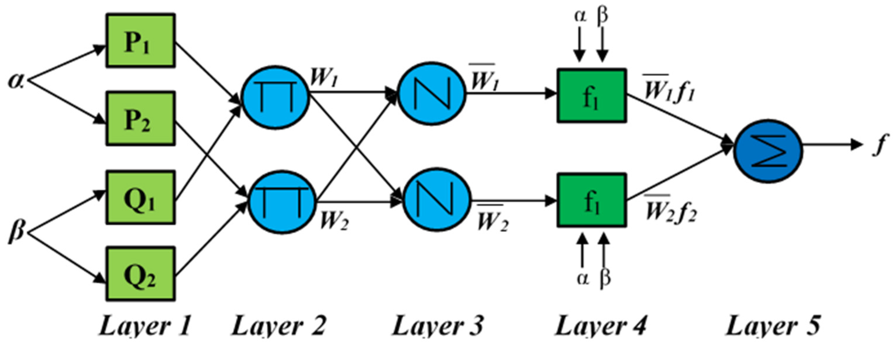
2.2.2. Adaptive Neuro-Fuzzy Inference System (ANFIS)

ANFIS, a variant of fuzzy inference systems (FIS), is adaptive in nature, incorporating fuzziness and ambiguity of input variables in developing input–output relationships of nonlinear systems [93]. An ANFIS grab holds the advantageous features of both the artificial neural networks and fuzzy set theory into an adaptive framework to model nonlinear and complex systems quite efficiently and effectively [94,95]. Due to less complexity and better learning ability [93], a Sugeno-type FIS is used to develop the ANFIS model utilizing a fuzzy c-means clustering (FCM) [96] algorithm to reduce the dimensionality of input variables. Detailed descriptions of ANFIS model structures are provided in Jang et al. [93] and are not repeated in this effort. Figure 2 presents an ANFIS model structure derived from a Sugeno-type FIS. The ANFIS models were developed in a MATLAB [97] environment.

2.2.3. Gaussian Process Regression (GPR)

A GPR is a nonparametric modeling algorithm that is derived from the theories of probability and Gaussian process [99]. Following a Gaussian distribution, a GPR model provides the output, $\mathrm{Y}$ from the input variables, and $\mathrm{X}\left(\mathrm{i}\right)$ through developing a functional relationship, which can be mathematically represented as [100]

$$\mathrm{Y}=\mathrm{f}\left(\mathrm{X}\left(\mathrm{i}\right)\right)+\mathsf{\epsilon }$$

(2)

where $\epsilon$ is a Gaussian noise, the variance of which is denoted by ${\mathsf{\sigma }}_{\mathrm{n}}^2$.

The mean, $\mathrm{m}\left({\mathrm{x}}_{\mathrm{i}}\right)$, and covariance, $\mathrm{k}\left({\mathrm{x}}_{\mathrm{i}},{\mathrm{x}}_{\mathrm{j}}\right)$, functions are the two important functional components of a typical GPR model. They can be mathematically expressed as [99]

$$\mathrm{m}\left({\mathrm{x}}_{\mathrm{i}}\right)=\mathrm{E}\left[\mathrm{f}\left({\mathrm{x}}_{\mathrm{i}}\right)\right]$$

(3)

$$\mathrm{k}\left({\mathrm{x}}_{\mathrm{i}},{\mathrm{x}}_{\mathrm{j}}\right)=\mathrm{E}\left[\left(\mathrm{f}\left({\mathrm{x}}_{\mathrm{i}}\right)-\mathrm{m}\left({\mathrm{x}}_{\mathrm{i}}\right)\right)\left(\mathrm{f}\left({\mathrm{x}}_{\mathrm{j}}\right)-\mathrm{m}\left({\mathrm{x}}_{\mathrm{j}}\right)\right)\right]$$

(4)

On the basis of these two key functions, the functional relationship using Gaussian process theory is established by the following equation:

$$\mathrm{f}\left(\mathrm{x}\right)~\mathrm{gp}\left(\mathrm{m}\left({\mathrm{x}}_{\mathrm{i}}\right),\mathrm{k}\left({\mathrm{x}}_{\mathrm{i}},{\mathrm{x}}_{\mathrm{j}}\right)\right)$$

(5)

The prediction probability distribution of a GPR model is governed by the free parameters or hyperparameters, which are in essence the parameters of the mean and covariance functions. The values of free parameters or hyperparameters depend on the training dataset’s log-likelihood function values. The GPR models were developed by utilizing the commands and functions of MATLAB [97].

2.2.4. M5 Model Trees (M5 Tree)

The development of the M5 tree is derived from the philosophies associated with the M5 technique [101,102] in building standalone trees. The prediction capabilities of M5 trees were demonstrated and well documented in various research domains [103,104]. In the M5 tree modeling approach, a complex modeling task is sub-divided into numerous sub-tasks via the divide-and-conquer technique, and the final result is the integration of solutions from all the sub-tasks [103]. This splitting technique results in a hierarchy of model trees in which non-terminal nodes are associated with splitting rules, whereas expert models are represented by the tree leaves [104]. Model development using the M5 tree technique is performed using three stepwise procedures: (1) development of an initial tree, (2) pruning of the tree, and (3) smoothing of the tree [105]. In the MATLAB environment, a toolbox “M5PrimeLab” [106] was used to develop M5 trees for predicting daily reference ET₀ values.

2.2.5. Multivariate Adaptive Regression Spline (MARS)

MARS [107] is a nonparametric modeling technique that is adaptive in nature and is believed to be a flexible and rapid approach to developing regression models. The MARS approach partitions the entire decision space into several input parameters on which standalone basis functions or splines are fitted to obtain the final MARS model [108]. Both a forward procedure and a backward procedure are utilized, i.e., MARS initially builds a comparatively complex model using the user-specified maximum number of basis functions in the forward step. In contrast, in the backward step, MARS parsimoniously selects the most significant input variables in predicting the output variable [109]. The backward step eliminates redundant input variables and assists in simplifying the final model while avoiding over-or under-fitting. The relationship between the input and output variables can be represented by the following equation [110]:

$${\mathrm{BF}}_{\mathrm{i}}\left(\mathrm{x}\right)=\max \left(0,{\mathrm{x}}_{\mathrm{j}}-\mathsf{\alpha }\right){ \mathrm{OR} \mathrm{BF}}_{\mathrm{i}}\left(\mathrm{x}\right)=\max \left(0,\mathsf{\alpha }-{\mathrm{x}}_{\mathrm{j}}\right)$$

(6)

$$\mathrm{y}=\mathrm{f}\left(\mathrm{x}\right)=\mathsf{\beta }\pm {\mathsf{\gamma }}_{\mathrm{k}}\times {\mathrm{BF}}_{\mathrm{i}}\left(\mathrm{x}\right)$$

(7)

where $\mathrm{i}$ represents the index of Basis functions, $\mathrm{j}$ denotes the index of input variables, ${\mathrm{BF}}_{\mathrm{i}}$ symbolizes the ${\mathrm{i}}^{\mathrm{th}}$ Basis function, ${\mathrm{x}}_{\mathrm{j}}$ is the ${\mathrm{j}}^{\mathrm{th}}$ input variable, $\mathsf{\alpha }$ is a threshold value used by the MARS model during model building, $\mathsf{\beta }$ is a constant, ${\mathsf{\gamma }}_{\mathrm{k}}$ indicates the respective coefficient of ${\mathrm{BF}}_{\mathrm{i}}\left(\mathrm{x}\right)$, and $\mathrm{y}$ denotes the model prediction (output variable).

A MATLAB toolbox ‘ARESLab’ [106] was employed to build MARS-based ET₀ prediction models. This study used both piecewise-linear and piecewise-cubic modeling approaches to predict daily ET₀ values.

2.2.6. Probabilistic Linear Regression (PLR)

PLR utilizes Bayesian inference techniques to develop prediction models through probabilistically performing linear regression. The PLR approach is often referred to as empirical Bayesian linear regression, using either an expectation-maximization (EM) algorithm [111] or a Mackay fixpoint iteration method [112]. The EM algorithm is generally utilized to formulate the PLR models. As such, the present study used the EM algorithm in developing PLR-based ET₀ prediction models. Mo Chen [113] developed a MATLAB toolbox in this research to develop PLR models.

2.2.7. Support Vector Regression (SVR)

SVRs are derived from the principles of the support vector machine (SVM) algorithm [114], which has been attaining significant attention in recent years for its capability to solve a diversified range of regression and classification problems [115]. SVRs are developed via a nonlinear mapping technique that utilizes required data from the input space to a high-dimensional feature space on which linear regressions are executed [116]. An elaborated explanation of the theory of the SVR approach has been provided in Chevalier et al. [117], and only a brief account of the SVR theorem is presented in this effort. The following equation symbolizes the training dataset in developing a linear SVR model:

$$\left\{\left(\overline{{\mathrm{x}}_1},{ \mathrm{y}}_1\right),\left(\overline{{\mathrm{x}}_2},{ \mathrm{y}}_2\right),\dots ,\left(\overline{{\mathrm{x}}_{\mathrm{l}}},{ \mathrm{y}}_{\mathrm{l}}\right)\right\}$$

(8)

$$\overline{{\mathrm{x}}_{\mathrm{i}}}\in {\mathrm{R}}^{\mathrm{d}},{ \mathrm{y}}_{\mathrm{i}}\in \mathrm{R}, \mathrm{and\; l\; =\; number\; of\; data\; entries}$$

In this case, the solution function can be expressed as

$$\mathrm{f}\left(\overline{\mathrm{x}}\right)={\displaystyle \sum }_{\mathrm{i}=1}^{\mathrm{l}}\left({\mathsf{\alpha }}_{\mathrm{i}}-{\mathsf{\alpha }}_{\mathrm{i}}^{*}\right)<\overline{{\mathrm{x}}_{\mathrm{i}}},\overline{\mathrm{x}}>+\mathrm{b}$$

(9)

where $<.,.>$ denotes dot product, and ${\mathsf{\alpha }}_{\mathrm{i}}$, ${\mathsf{\alpha }}_{\mathrm{i}}^{*}$, and $\mathrm{b}$ represent coefficients computed by the SVR model.

A data transformation step is performed to build nonlinear SVR models, including a nonlinear mapping function $\varnothing$ [118] that transforms low-dimensional input space into a high-dimensional feature space. The computation $\varnothing$ becomes challenging during progressive mapping of the input–output data into higher dimensions. This limitation is handled using the Mercers theorem, which can be represented by the following equation:

$$<\varnothing \left(\overline{\mathrm{u}}\right),\varnothing \left(\overline{\mathrm{v}}\right)>=\mathrm{k}\left(\overline{\mathrm{u}},\overline{\mathrm{v}}\right)$$

(10)

For a particular mapping $\varnothing$, the Mercers theorem introduces the concept of using a kernel function $\mathrm{k}$, which is used to calculate the dot product of any two points ($\overline{\mathrm{u}},\overline{\mathrm{v}}$), and the computation of dot products in this approach bypasses the explicit calculation of high-dimensional and nonlinear mapping. The prediction performance of nonlinear SVR models depends on the kernel function, which is regarded as one of the most important parameters in SVR modeling.

2.3. Ranking of the ET₀ Prediction Models: Shannon’s Entropy

ET₀ prediction models were ranked using performance-based weights assigned to standalone models using Shannon’s entropy principle. For this, a decision matrix of prediction models ($\mathrm{m}$) and performance indices ($\mathrm{PI})$ is formulated, which can be represented in the form of the following equation [119]:

$${\mathrm{ET}}_{\mathrm{ij}}=\left[\begin{array}{ccc}\begin{array}{c}{\mathrm{ET}}_{11}\\ {\mathrm{ET}}_{12}\\ \begin{array}{c}⋮\\ {\mathrm{ET}}_{1\mathrm{PI}}\end{array}\end{array}& \begin{array}{c}{\mathrm{ET}}_{21}\\ {\mathrm{ET}}_{22}\\ \begin{array}{c}⋮\\ {\mathrm{ET}}_{2\mathrm{PI}}\end{array}\end{array}& \begin{array}{cc}\begin{array}{c}\cdots \\ \cdots \\ \begin{array}{c}⋮\\ \cdots \end{array}\end{array}& \begin{array}{c}{\mathrm{ET}}_{\mathrm{m}1}\\ {\mathrm{ET}}_{\mathrm{m}2}\\ \begin{array}{c}⋮\\ {\mathrm{ET}}_{\mathrm{mPI}}\end{array}\end{array}\end{array}\end{array}\right]$$

(11)

To reduce the adverse impacts of index dimensionality, we standardized the performance index values between 0 and 1$\{{\mathrm{S}}_{\mathrm{ij}}\in \left[0,1\right], \mathrm{i}=1,2,\dots ,\mathrm{m};\mathrm{j}=1,2,\dots ,\mathrm{PI}\}$. The standardization component ${\mathrm{S}}_{\mathrm{ij}}$ was performed using the following equation [119]:

$${\mathrm{S}}_{\mathrm{ij}}=\{\begin{array}{cc}\frac{{\mathrm{ET}}_{\mathrm{ij}}}{\max \left({\mathrm{ET}}_{\mathrm{i}1},{\mathrm{ET}}_{\mathrm{i}2},\dots ,{\mathrm{ET}}_{\mathrm{iPI}}\right)},& \mathrm{for} \mathrm{benefit} \mathrm{indexes}\\ \frac{{\mathrm{X}}_{\mathrm{ij}}}{\min \left({\mathrm{ET}}_{\mathrm{i}1},{\mathrm{ET}}_{\mathrm{i}2},\dots ,{\mathrm{ET}}_{\mathrm{iPI}}\right)},& \mathrm{for} \cos \mathrm{t} \mathrm{indexes}\end{array}$$

(12)

Shannon’s entropy-based ranking was performed using a five-step stepwise procedure described in Roy et al. [21], which was not repeated here.

2.4. Selection of Input Variables for Daily Predictions

All possible combinations of the five input variables (minimum temperatures, maximum temperatures, relative humidity, wind speed, and sunshine hours) were used. A total of 31 models were developed on the basis of the 31 combinations (single, two-input combinations, three-input combinations, four-input combinations, and all five inputs) of input variables. Two-, three-, and four-input combinations are presented in

Table 4. Different combinations of two-, three-, and four-input combinations.

Two-Input Combinations	Three-Input Combinations	Four-Input Combinations
Min temp, max temp	Min temp, max temp, humidity	Min temp, max temp, humidity, wind speed
Min temp, humidity	Min temp, max temp, wind speed	Min temp, max temp, humidity, sunshine hours
Min temp, wind speed	Min temp, max temp, sunshine hours	Min temp, max temp, wind speed, sunshine hours
Min temp, sunshine hours	Min temp, humidity, wind speed	Min temp, humidity, wind speed, sunshine hours
Max temp, humidity	Min temp, humidity, sunshine hours	Max temp, humidity, wind speed, sunshine hours
Max temp, wind speed	Min temp, wind speed, sunshine hours
Max temp, sunshine hours	Max temp, humidity, wind speed
Humidity, wind speed	Max temp, humidity, sunshine hours
Humidity, sunshine hours	Max temp, wind speed, sunshine hours
Wind speed, sunshine hours	Humidity, wind speed, sunshine hours

.

These combinations of input variables were evaluated for two deep learning algorithms (LSTM and Bi-LSTM). The 62 models (31 LSTM + 31 Bi-LSTM) developed were ranked on the basis of their prediction accuracies using Shannon’s entropy by incorporating a number of benefit (correlation coefficient, Nash–Sutcliffe efficiency coefficient, Willmott’s index of agreement) and cost (normalized or relative root mean squared error, maximum absolute error, median absolute deviation) performance evaluation indices. The best-input combinations thus obtained were used to develop the other shallow machine learning algorithms.

2.5. Model Performance Evaluation

The performances of the proposed models were evaluated using various statistical evaluation indices as follows:

-

Correlation coefficient, R

$$\mathrm{R}=\frac{{{\displaystyle \sum }}_{\mathrm{i}=1}^{\mathrm{n}}\left({\mathrm{ET}}_{\mathrm{i},\mathrm{a}}-\overline{{\mathrm{ET}}_{\mathrm{a}}}\right)\left({\mathrm{ET}}_{\mathrm{i},\mathrm{a}}-\overline{{\mathrm{ET}}_{\mathrm{p}}}\right)}{\sqrt{{{\displaystyle \sum }}_{\mathrm{i}=1}^{\mathrm{n}}{\left({\mathrm{ET}}_{\mathrm{i},\mathrm{a}}-\overline{{\mathrm{ET}}_{\mathrm{a}}}\right)}^2}\sqrt{{{\displaystyle \sum }}_{\mathrm{i}=1}^{\mathrm{n}}{\left({\mathrm{ET}}_{\mathrm{i},\mathrm{p}}-\overline{{\mathrm{ET}}_{\mathrm{p}}}\right)}^2}}$$

(13)

-

Nash–Sutcliffe efficiency coefficient, NS [120]

$$\mathrm{NS}=1-\frac{{{\displaystyle \sum }}_{\mathrm{i}=1}^{\mathrm{n}}{\left({\mathrm{ET}}_{\mathrm{i},\mathrm{a}}-{\mathrm{ET}}_{\mathrm{i},\mathrm{p}}\right)}^2}{{{\displaystyle \sum }}_{\mathrm{i}=1}^{\mathrm{n}}{\left({\mathrm{ET}}_{\mathrm{i},\mathrm{a}}-\overline{{\mathrm{ET}}_{\mathrm{a}}}\right)}^2}$$

(14)

-

Index of agreement, IOA [121]

$$\mathrm{IOA}=1-\frac{{{\displaystyle \sum }}_{\mathrm{i}=1}^{\mathrm{n}}{\left({\mathrm{ET}}_{\mathrm{i},\mathrm{a}}-{\mathrm{ET}}_{\mathrm{i},\mathrm{p}}\right)}^2}{{{\displaystyle \sum }}_{\mathrm{i}=1}^{\mathrm{n}}{\left(\left|{\mathrm{ET}}_{\mathrm{i},\mathrm{p}}-\overline{{\mathrm{ET}}_{\mathrm{a}}}\right|+\left|{\mathrm{ET}}_{\mathrm{i},\mathrm{a}}-\overline{{\mathrm{ET}}_{\mathrm{a}}}\right|\right)}^2}$$

(15)

-

Root mean square error, RMSE [122]

$$\mathrm{RMSE}=\sqrt{\frac{1}{\mathrm{n}}{\displaystyle \sum }_{\mathrm{i}=1}^{\mathrm{n}}{\left({\mathrm{ET}}_{\mathrm{i},\mathrm{a}}-{\mathrm{ET}}_{\mathrm{i},\mathrm{p}}\right)}^2}$$

(16)

-

Normalized RMSE, NRMSE

$$\mathrm{NRMSE}=\frac{\mathrm{RMSE}}{\overline{{\mathrm{ET}}_{\mathrm{a}}}}$$

(17)

-

Maximum absolute error, MAE

$$\mathrm{MAE}=\max \left[\left|{\mathrm{ET}}_{\mathrm{i},\mathrm{a}}-{\mathrm{ET}}_{\mathrm{i},\mathrm{p}}\right|\right]$$

(18)

-

Median absolute deviation, MAD

$$\begin{gathered} \mathrm{MAD}\left({\mathrm{ET}}_{\mathrm{a}},{\mathrm{ET}}_{\mathrm{p}}\right)=\mathrm{median}\left(\left|{\mathrm{ET}}_{1,\mathrm{a}}-{\mathrm{ET}}_{1,\mathrm{p}}\right|,\left|{\mathrm{ET}}_{2,\mathrm{a}}-{\mathrm{ET}}_{2,\mathrm{p}}\right|,\dots , \left|{\mathrm{ET}}_{\mathrm{n},\mathrm{a}}-{\mathrm{ET}}_{\mathrm{n},\mathrm{p}}\right|\right) \\ \mathrm{for} \mathrm{i}=1,2,\dots ,\mathrm{n} \end{gathered}$$

(19)

where ${\mathrm{ET}}_{\mathrm{i},\mathrm{a}}$ and ${\mathrm{ET}}_{\mathrm{i},\mathrm{p}}$ are ${\mathrm{ET}}_0$ quantities at the ${\mathrm{i}}^{\mathrm{th}}$ data points acquired from the FAO-56 PM computed and model predicted values, respectively; $\overline{{\mathrm{ET}}_{\mathrm{a}}}$ represents the arithmetic mean of the FAO-56 PM computed ${\mathrm{ET}}_0$ values; and $\mathrm{n}$ is the amount of input–output data.

3. Results and Discussion

3.1. Daily Prediction of ET₀ Using Various Machine Learning Algorithms at the Training Station (Gazipur Sadar)

To determine the optimum numbers of input variables combinations, we used 31 possible combinations of five input variables to develop 31 LSTM and 31 Bi-LSTM models. Learning (training) and testing of the ET₀ models were performed simultaneously. Prediction errors on the test dataset in terms of RMSE criterion for the 31 developed models are presented in

Table 5. Prediction errors of deep learning-based ET₀ models (LSTM and Bi-LSTM) with different input combinations on the test dataset.

Model No.	Different Input Combinations	Test RMSE, mm/d
		LSTM	Bi-LSTM
Single Input Combinations
M1	Min temp	0.880	0.964
M2	Max temp	0.775	0.781
M3	Humidity	1.124	1.211
M4	Wind speed	1.177	1.105
M5	Sunshine hours	0.732	0.807
Two Inputs combinations
M6	Min temp, max temp	0.765	0.779
M7	Min temp, humidity	0.729	0.751
M8	Min temp, wind speed	1.004	1.049
M9	Min temp, sunshine hours	0.527	0.514
M10	Max temp, humidity	0.634	0.602
M11	Max temp, wind speed	0.734	0.743
M12	Max temp, sunshine hours	0.501	0.430
M13	Humidity, wind speed	0.727	0.760
M14	Humidity, sunshine hours	0.531	0.983
M15	Wind speed, sunshine hours	0.527	0.627
Three Inputs Combinations
M16	Min temp, max temp, humidity	0.570	0.574
M17	Min temp, max temp, wind speed	0.729	0.722
M18	Min temp, max temp, sunshine hours	0.512	0.447
M19	Min temp, humidity, wind speed	0.726	0.723
M20	Min temp, humidity, sunshine hours	0.337	0.377
M21	Min temp, wind speed, sunshine hours	0.470	0.501
M22	Max temp, humidity, wind speed	0.567	0.566
M23	Max temp, humidity, sunshine hours	0.300	0.239
M24	Max temp, wind speed, sunshine hours	0.409	0.394
M25	Humidity, wind speed, sunshine hours	0.337	0.333
Four Inputs Combinations
M26	Min temp, max temp, humidity, wind speed	0.577	0.561
M27	Min temp, max temp, humidity, sunshine hours	0.262	0.229
M28	Min temp, max temp, wind speed, sunshine hours	0.382	0.404
M29	Min temp, humidity, wind speed, sunshine hours	0.271	0.238
M30	Max temp, humidity, wind speed, sunshine hours	0.107	0.116
All Inputs
M31	Min temp, max temp, humidity, wind speed, sunshine hours	0.081	0.087

RMSE = root mean squared error, LSTM = long short-term memory networks, Bi-LSTM = bi-directional long-short term memory networks. The numbers in boldface indicate the best performance, whereas the numbers in boldface and italicized represent the worst performance.

. As evidenced by the numerical values presented in Table 5, the LSTM model predictions were slightly better than those of the Bi-LSTM models when the RMSE criterion was used as a deciding factor. It was also observed that both the LSTM- and Bi-LSTM-based ET₀ prediction models produced the lowest RMSE values (best daily ET₀ predictions) when all five variables were used. The performance of LSTM (RMSE = 0.081 mm/d) was slightly better than that of the Bi-LSTM (RMSE = 0.087 mm/d) model. However, in situations where adequate data are not available, the use of fewer input variables may be employed to achieve a realistically precise prediction of ET₀ values. For instance, four climatological variables (a combination of maximum temperature, relative humidity, wind speed, and sunshine hours) could be used to obtain sufficiently accurate daily ET₀ predictions using LSTM (test error in terms of RMSE value equals 0.107 mm/d) and Bi-LSTM (test error in terms of RMSE value equals 0.116 mm/d) models. Other combinations of four meteorological variables, e.g., (minimum temperature, maximum temperature, relative humidity, sunshine hours) and (minimum temperature, relative humidity, wind speed, sunshine hours) provided reasonably accurate daily ET₀ predictions (Table 5). In addition, combinations of three meteorological variables (relative humidity, wind speed, sunshine hours) and (minimum temperature, relative humidity, sunshine hours) produced reasonable accurate predictions, with test RMSE values ranging between 0.333 and 0.377 mm/d.

Nonetheless, decision making in such situations is challenging, as the RMSE criterion alone is insufficient as a decision-making tool. To assist in the decision-making process, we used three benefit (the higher numeric values indicate better model performances: R, NS, IOA) and three cost (the lower the numeric values, the better the model performance: NRMSE, MAE, MAD) performance evaluation indices in the decision-making process with the aid of Shannon’s entropy. On the testing dataset, we computed the R, NS, IOA, NRMSE, MAE, and MAD criteria for all 31 LSTM and 31 Bi-LSTM models. These evaluation indices were used to rank proposed models using Shannon’s entropy-based decision theory.

Table 6. Ranking of the LSTM and Bi-LSTM models using Shannon’s entropy.

Sl. No.	LSTM		Bi-LSTM
	Model	Ranking Value	Model	Ranking Value
1	M31	0.996	M31	0.966
2	M30	0.906	M30	0.913
3	M27	0.702	M27	0.704
4	M23	0.687	M23	0.696
5	M20	0.657	M29	0.688
6	M29	0.652	M25	0.642
7	M25	0.640	M20	0.621
8	M28	0.604	M24	0.600
9	M24	0.600	M28	0.594
10	M21	0.584	M12	0.581
11	M12	0.563	M18	0.576
12	M18	0.561	M21	0.563
13	M14	0.560	M26	0.557
14	M22	0.558	M9	0.555
15	M26	0.556	M22	0.551
16	M15	0.555	M16	0.551
17	M9	0.555	M10	0.535
18	M16	0.554	M15	0.522
19	M10	0.535	M17	0.488
20	M11	0.496	M19	0.485
21	M17	0.493	M11	0.482
22	M19	0.491	M7	0.478
23	M13	0.491	M13	0.475
24	M7	0.483	M6	0.462
25	M5	0.482	M2	0.460
26	M6	0.470	M5	0.451
27	M2	0.470	M14	0.384
28	M1	0.415	M1	0.376
29	M8	0.364	M8	0.336
30	M3	0.306	M4	0.311
31	M4	0.209	M3	0.256

shows the ranking results together with the corresponding ranking values.

It is perceived from the results presented in Table 6 that models that used all five input variables (M31) were the top-ranked predictors, followed by M30, M27, and M23 for both LSTM and Bi-LSTM algorithms. Models M3 and M4 appeared to be the worst performers when using LSTM or Bi-LSTM algorithms for model development. The findings are in accordance with the work of Kisi et al. [37], who indicated that considering all input variables greatly increased the accuracy of the prediction model (radial basis M5Tree) for the data acquired from the three weather stations. Therefore, the results suggest that all input variables would be employed to better predict the daily ET₀ for the meteorological data and the corresponding ET₀ values presented in this study. Consequently, to arrange for an impartial comparison, we developed other prediction modeling algorithms (ANFIS, GPR, M5Tree, MARS, PLR, and SVR) using all five input variables available for the study area. Similar evaluation indices were computed for all the other prediction modeling algorithms proposed in this research. The prediction results are presented in

Table 7. Performance indices of the developed ET₀ prediction models for the testing dataset.

Model	Performance Evaluation Indices
	R	NS	IOA	NRMSE	MAE, mm/d	MAD, mm/d
LSTM	0.998	0.995	0.999	0.021	0.666	0.025
Bi-LSTM	0.998	0.995	0.999	0.023	0.582	0.027
ANFIS	0.991	0.981	0.995	0.043	0.706	0.061
GPR	0.993	0.985	0.996	0.038	0.650	0.052
M5 Tree	0.985	0.970	0.993	0.054	1.153	0.062
MARS_C	0.992	0.983	0.996	0.041	0.869	0.054
MARS_L	0.992	0.983	0.996	0.040	0.760	0.054
PLR	0.973	0.943	0.985	0.075	1.489	0.114
SVR	0.993	0.985	0.996	0.038	0.676	0.050

MARS_C = piecewise cubic, MARS_L = piecewise linear.

.

The prediction results in Table 7 indicated that all ET₀ prediction models are reasonably accurate at predicting daily ET₀ values, as evidenced by the different performance indices computed on the testing dataset. While no standalone model exhibited the best performance for all evaluation indices, the individual prediction models provided the estimates of daily ET₀ values superior to others. All ET₀ models had satisfactory prediction accuracy as all models had better (higher) values R, NS, and IOA and lower NRMSE, MAE, and MAD values. LSTM and Bi-LSTM models had superior performance in comparison with others according to all performance evaluation indices. PLR was found to be the worst-performing model.

To provide an additional evaluation regarding the prediction capabilities of the proposed machine learning algorithms (ET₀ prediction models), we presented and compared the absolute error boxplots. Figure 3 illustrates the absolute error boxplots for all the developed models. Absolute error boxplots represent a relative assessment of the statistical distributions of the absolute errors between the FAO-56 PM-computed and model-predicted ET₀ values and supports the evaluation of the degree of general distributions of the inaccuracies provided by the models. The horizontal lines inside the boxplots represent the median values of the absolute errors, whereas the black circles mark the mean (average) of the absolute errors. Absolute error boxplots also demonstrated the superior performance of the LSTM- and Bi-LSTM-based models.

As far as the two best models are considered, the LSTM model performed better than Bi-LSTM when NRMSE and MAD criteria were considered. In contrast, Bi-LSTM outperformed the LSTM model according to the MAE criterion. On the other hand, both LSTM and Bi-LSTM performed equally well with respect to R, NS, and IOA criteria. Therefore, it is concluded that ET₀ prediction models showed differing precisions depending on the model evaluation indices calculated on the FAO-56 PM and model predicted ET₀ values, which indicated an inconsistency in the model performance when divergent or non-identical evaluation indices were employed. Decision making in this situation is extremely arduous and can be smoothed by employing a decision theory that integrates a number of different model evaluation indices in decision making. This study employed Shannon’s entropy as a decision-making tool.

The ranking of the proposed ET₀ models computed using Shannon’s entropy is presented in

Table 8. Shannon’s entropy values for different models and their corresponding ranks.

Model	Shannon’s Entropy Value	Rank
LSTM	0.979	1
Bi-LSTM	0.978	2
ANFIS	0.807	6
GPR	0.839	3
M5 tree	0.734	8
MARS_C	0.794	7
MARS_L	0.810	5
PLR	0.665	9
SVR	0.836	4

. The greater the values of Shannon’s entropy, the better the model’s performance. Table 8 suggests that LSTM was the top-performing model followed by Bi-LSTM, although the difference between the ranking values of these two models was negligible.

The performance index values for the best model (LSTM) are as follows (Table 7): R = 0.998, NS = 0.995, IOA = 0.999, NRMSE = 0.021, MAE = 0.666 mm/d, and MAD = 0.025 mm/d. Although an explicit comparison between the findings of this research and other studies is not possible due to variations in study conditions (modeling tools and geographical locations), the numeric values of various performance indices were observed as being comparable to or even better than those found in the recent literature on ET₀ modeling. For instance, the present study’s findings are superior to those obtained by Tao et al. [123], who obtained NRMSE and R² values of 0.043 and 0.97, respectively, using an optimization algorithm-tuned ANFIS model to predict ET₀ in the Bur Dedougou, Burkina Faso. The LSTM model proposed in this study also shows better performance than the optimization algorithm tuned SVR model developed in Ahmadi et al. [32], who obtained the following performance indices at various stations: RMSE = 0.540 mm/d and R = 0.983 at Mashhad station; RMSE = 0.404 mm/d and R = 0.980 at Arak station; RMSE = 0.299 mm/d and R = 0.989 at Shiraz station; RMSE = 0.559 mm/d and R = 0.978 at Tehran station; RMSE = 0.457 mm/d and R = 0.962 at Bandar Abbas station; and RMSE = 0.399 mm/d and R = 0.986 at Yazd station. The present study’s findings are also in good agreement with the findings presented in Chia et al. [124], who obtained RMSE and R² values of 0.001–0.197 mm/d and 1.000–0.949, respectively, at three stations using an optimization algorithm-tuned ELM model. The findings are also compared with those presented in Mohammadi and Mehdizadeh [125] that are based on RMSE and R² criteria. Our proposed LSTM model shows superior performance over the best models developed with the daily data in Ferreira and da Cunha [80], who reported NS values of 0.69 to 0.84 and R² values of 0.79 to 0.88. The present study’s findings are superior to the optimization algorithm-tuned ELM model developed by Wu et al. [30] that reported R² and NRMSE values of 0.993 and 0.0554, respectively. Elbeltagi et al. [126] reported R values of 0.94, 0.95, and 0.95 at the Ad Daqahliyah, Kafr ash Shaykh, and Ash Sharqiyah regions, respectively, using the DNN model. These R values were lower than the R-value obtained using the proposed LSTM model in the present study (R = 0.998). The NS value of the present study (NS = 0.995) is also superior to the NS value (NS = 0.959) presented in Gao et al. [127], indicating the better performance of the proposed LSTM model. The findings of our study are also comparable to those presented in Chia et al. [50], who reported minimum MAE and RMSE values of 0.444 mm/d and 0.543 mm/d, respectively.

Nevertheless, an apple-to-apple comparison can be performed between the findings obtained from the LSTM model presented in this effort with the models investigated in Roy et al. [21] (an ensemble of ANFIS models) and in Roy et al. [20] (optimization algorithm tuned ANFIS model). With the optimization algorithm-tuned ANFIS model for the same study area, Roy et al. [20] obtained the following performance indices: R = 0.993, NS = 0.986, IOA = 0.996, MAD = 0.054 mm/d, NRMSE = 0.038. Our proposed LSTM model performed better than the ANFIS model presented by Roy et al. [20] with respect to all of these performance indices (R = 0.998, NS = 0.995, IOA = 0.999, NRMSE = 0.021, and MAD = 0.025 mm/d in the present study). Statistical indices provided by the LSTM model (R = 0.998, NS = 0.995, IOA = 0.999, and MAD = 0.025 mm/d) proposed in this research also appeared to be superior than those presented by Roy et al. [21] using ensemble of ANFIS models (R = 0.993, NS = 0.985, IOA = 0.996, and MAD = 0.054 mm/d). Furthermore, the proposed LSTM model’s performance is superior to the performance of the optimization algorithm tune hierarchical fuzzy systems (HFS) presented by Roy et al. [46] with respect to R (LSTM = 0.998, HFS = 0.987), NRMSE (LSTM = 0.021, HFS = 0.052), and MAD (LSTM = 0.025 mm/d, HFS = 0.068 mm/d) criteria.

3.2. One-Step-Ahead Prediction of ET₀ Using Different Modeling Approaches at the Training Station (Gazipur Sadar)

3.2.1. One-Step-Ahead Forecast Using Sequence to Sequence Regression LSTM (SSR-LSTM) Network

An SSR-LSTM network-based model was trained by employing the historical ET₀ dataset (time series) computed using the FAO-56 PM equation from the meteorological variables. In an SSR-LSTM model, the outputs from the model correspond to the training sequences (ET₀ time series) with ET₀ values moved to a one-time step ahead. At every time step of the ET₀ sequence, an SSR-LSTM network learns how to predict ET₀ values for the next time step. For training the proposed SSR-LSTM model, the historical ET₀ time series was partitioned into training and test sets (90% of the entire data was used for training, whereas the remaining 10% was used for testing the model). Model parameters including the number of hidden layers and neurons were decided upon by conducting several trials. An SSR-LSTM model with one hidden layer having 200 hidden neurons in the hidden layer provided the best results for both the model training and testing phases. The optimal values of other model parameters were solver = ‘adam’, number of epochs = 250, gradient threshold = 1, initial learning rate = 0.005, and multiplying factor for the learn rate dropping = 0.2. Model performance is presented in Figure 4.

It is observed from Figure 4 that even though the SSR-LSTM model adequately apprehended the trends of the ET₀ time series for the test set of the data (Figure 4b), the SSR-LSTM forecasts were comparatively flat compared to the original ET₀ time-series data (Figure 4a). This necessitates the improvement in the forecasting performance of the initial SSR-LSTM model. One way of improving performance is to update the SSR-LSTM network state using the observed ET₀ values instead of the predicted ET₀ values. Resetting the network’s state is used in this study to prevent previous predictions from impacting the results.

This was performed by resetting the network state in order to prevent previous predictions from affecting the predictions on the new dataset. The forecasting results obtained from the updated network state of the SSR-LSTM model are presented in Figure 5.

3.2.2. One-Step-Ahead Forecast Using ANFIS, LSTM, and Bi-LSTM Models

For developing ANFIS, LSTM, and Bi-LSTM models to provide one-step-ahead forecasts, we computed PACF functions to obtain time-lagged information from the daily ET₀ time series. This information obtained from the PACF functions was employed to assess the time-based dependences between ET₀ for a present day (${\mathrm{ET}}_{\mathrm{t}}$) and the ET₀ values at a particular day in a prior period (e.g., at a lag time of ${\mathrm{ET}}_{\mathrm{t}-1},{ \mathrm{ET}}_{\mathrm{t}-2},{ \mathrm{ET}}_{\mathrm{t}-3},{ \mathrm{ET}}_{\mathrm{t}-4},{ \mathrm{and} \mathrm{ET}}_{\mathrm{t}-5}$). These time-based dependences in the ET₀ time series were assessed for 50 time lags (e.g., ${\mathrm{ET}}_{\mathrm{t}-1}$ to ${\mathrm{ET}}_{\mathrm{t}-50}$), as shown in Figure 6. In Figure 6, the blue lines indicate the 95% confidence band, whereas the red vertical lines represent the corresponding values of ACF and PACF. Time-lagged ET₀ values serve as the inputs to the ANFIS, LSTM, and Bi-LSTM models to forecast one-day-ahead ET₀ values (outputs from the models). The optimal sets of time-lagged ET₀ inputs for model development were selected carefully after observing the PACF functions.

A careful observation of the PACF plot shown in Figure 6 determines the following time-lagged ET₀ values as inputs to the developed models:

$${\mathrm{ET}}_{\mathrm{t}},{ \mathrm{ET}}_{\mathrm{t}-1},{ \mathrm{ET}}_{\mathrm{t}-2},{ \mathrm{ET}}_{\mathrm{t}-3},{ \mathrm{ET}}_{\mathrm{t}-4},{ \mathrm{ET}}_{\mathrm{t}-5},{ \mathrm{ET}}_{\mathrm{t}-6},{ \mathrm{ET}}_{\mathrm{t}-7},{ \mathrm{ET}}_{\mathrm{t}-8},{ \mathrm{ET}}_{\mathrm{t}-9},{ \mathrm{ET}}_{\mathrm{t}-10},{ \mathrm{ET}}_{\mathrm{t}-11}$$

The outputs from the developed models were ${\mathrm{ET}}_{\mathrm{t}+1}$(one-day-ahead ET₀ values).

ANFIS outputs: The results of the one-step-ahead forecast using the ANFIS model are presented in Figure 7 and

Table 9. Performance indices of the one-day-ahead ET₀ prediction models for the testing dataset.

Model	Performance Evaluation Indices
	R	NS	IOA	NRMSE	MAE, mm/d	MAD, mm/d
ANFIS	0.755	0.567	0.858	0.207	2.710	0.308
Bi-LSTM	0.999	0.998	0.999	0.014	0.491	0.017
LSTM	0.698	0.429	0.833	0.237	3.047	0.334
SSR-LSTM	0.818	0.666	0.898	0.184	2.687	0.279

. Figure 7 presents ANFIS forecasts through scatter plots and hydrographs, whereas Table 8 shows model prediction capabilities based on several statistical performance evaluation indices. Hydrographs and scatterplots presented in Figure 7 demonstrate the reasonable precision of the one-day-ahead ET₀ forecasts by the ANFIS model. It is observed from Figure 7 that the training and test RMSE (0.759 and 0.789 mm/d, respectively, for the training and testing phases) did not vary considerably, which indicates a better model fit without model over- or under-fitting. Figure 7 also indicates acceptable values of training and test R-values (0.825 and 0.755, respectively, for the training and testing phases). As far as other performance evaluation indices are considered, the ANFIS model produced the following values of performance measures computed on the test dataset: NS = 0.567, IOA = 0.858, NRMSE = 0.207 mm/d, MAE = 2.710 mm/d, and MAD = 0.308 mm/d.

LSTM and Bi-LSTM outputs: Comparison of FAO-56 PM-calculated and model-predicted ET₀ values, error plots, and projected (one-step-ahead) ET₀ values produced by the LSTM and Bi-LSTM models are presented in Figure 8 and Figure 9, respectively. It is noticed from Figure 8 and Figure 9 that both LSTM and Bi-LSTM models captured the trend of the ET₀ time series precisely and that Bi-LSTM model forecasts were superior to those of the LSTM model. The performance evaluation results based on several statistical performance evaluation indices are presented in Table 9. The LSTM model produced the following values of performance measures computed on the test dataset: R = 0.698, NS = 0.698, IOA = 0.429, NRMSE = 0.237 mm/d, MAE = 3.047 mm/d, and MAD = 0.334 mm/d. On the other hand, the Bi-LSTM model produced the following values of performance measures computed on the test dataset: R = 0.999, NS = 0.998, IOA = 0.999, NRMSE = 0.014 mm/d, MAE = 0.491 mm/d, and MAD = 0.017 mm/d.

It is observed from Table 9 that the Bi-LSTM model provided a superior performance compared to the other models (SSR-LSTM, ANFIS, and LSTM) according to the statistical indices computed on the test dataset. It is noted that the prediction results with respect to the calculated performance indices did not demonstrate a considerable inconsistency. However, to reach a solid conclusion regarding the best-performing model, we applied the concept of Shannon’s entropy to provide a performance ranking (

Table 10. Shannon’s entropy-based model ranking for one-day-ahead ET₀ forecasts.

Model	Shannon’s Entropy Value	Rank
Bi-LSTM	1.00	1
SSR-LSTM	0.30	2
ANFIS	0.27	3
LSTM	0.24	4

). It is observed from Table 10 that Bi-LSTM appeared to be the best performer, while SSR-LSTM, ANFIS, and LSTM held the second, third, and fourth positions, respectively. Therefore, according to the performance results for one-step-ahead forecasting, the best-performing Bi-LSTM model was employed to provide multi-step (5 day)-ahead forecasting.

3.3. Multi-Step (5 Day-Ahead) Forecasting Using the Bi-LSTM Model

The forecasting performance of the developed ET₀ prediction model using the Bi-LSTM algorithm was evaluated using several statistical performance indices on the test dataset. However, to ascertain that no model over- or under-fitting occurred, we quantitatively evaluated the results obtained from both the training and validation phases. Five Bi-LSTM models were developed to forecast 1, 2, 3, 4, and 5 day-ahead ET₀ values. For all models, the selected time-lagged variables were served as inputs to the Bi-LSTM models.

Table 11. Training and validation performances of the developed Bi-LSTM models at Gazipur station.

Forecasting Horizon	Training RMSE, mm/d	Validation RMSE, mm/d
1 day	0.08	0.11
2 days	0.12	0.17
3 days	0.09	0.18
4 days	0.10	0.22
5 days	0.10	0.28

presents the performances of the developed Bi-LSTM models on the training and validation datasets. It is evident from Table 11 that the absolute variances between the training and validation performances increased with the increase in the forecasting horizon. Overall, the training performances were satisfactory for all forecasting horizons.

The trained and validated Bi-LSTM models were then used to forecast ET₀ values on the test dataset, which were selected from the entire dataset. Testing performances were assessed using several evaluation indices, as shown in

Table 12. Multi-day-ahead forecasting performance of the Bi-LSTM model on the test dataset at Gazipur station.

Indices	Forecasting Horizon
	1 Day	2 Days	3 Days	4 Days	5 Days
RMSE, mm/d	0.11	0.17	0.18	0.22	0.28
NRMSE	0.03	0.04	0.05	0.06	0.07
R	1.00	0.99	0.99	0.98	0.97
MAD, mm/d	0.03	0.04	0.04	0.06	0.08
MAE, mm/d	0.07	0.08	0.10	0.13	0.17
NS	0.99	0.98	0.98	0.97	0.95
IOA	1.00	0.99	0.99	0.99	0.99

. It is perceived from Table 12 that the forecasting horizon greatly influenced the forecasting accuracies. The accuracy decreased with the increase in the forecasting horizon as in the case of the training and validation performances. However, the overall performances of the Bi-LSTM model for all forecasting horizons showed particularly good performance, as indicated by the computed statistical performance evaluation indices. The performance of the developed models was also assessed using line graphs and error plots as shown in Figure 10.

It is observed from Table 12 that the Bi-LSTM model showed reasonably good performance, as evidenced by the computed performance indices. It produced lower values of cost indices (RMSE, NRMSE, MAD, and MAE) as well as higher values of benefit indices (R, NS, IOA). However, it is noted that the forecasting accuracy largely depended on the forecasting horizon, i.e., the sequence of forecasting accuracies are as follows: 1 day > 2 days > 3 days > 4 days > 5 days. This finding is in good agreement with the work of Yin et al. [128], who also stated that forecasting accuracy decreased with the increased forecasting horizon. Nevertheless, the forecasting accuracy of the Bi-LSTM model at 5 days ahead was also found acceptable for deep learning-based modeling of ET₀. Ferreira and da Cunha [82] also reported better deep learning model performance (CNN-LSTM) on the first and second forecasting days. Our findings using the Bi-LSTM model (RMSE = 0.11–0.28 mm/d) outperformed the CNN-LSTM model proposed by Ferreira and da Cunha [82] (mean RMSE values of 0.87 to 0.88 mm/d) with respect to RMSE criterion. Our proposed Bi-LSTM model performed better than the Bi-LSTM model proposed by Yin et al. [128] with respect to RMSE, R, and NS criteria. For instance, for 1 day-ahead forecasting, Yin et al. [128] obtained RMSE, R, and NS values of 0.159 mm/d, 0.992, and 0.988, respectively, whereas the values of RMSE, R, and NS in our study were found to be 0.11 mm/d, 1.00, and 0.99, respectively. Similarly, our proposed Bi-LSTM model outperformed the Bi-LSTM model presented by Yin et al. [128] for 4 day-ahead ET₀ forecasting. Moreover, our results also showed superior performance than the Bi-LSTM model results presented by Roy [81] in terms of R and IOA criteria for 1 day-ahead ET₀ forecasting. Roy [81] reported R and IOA values of 0.698 to 0.999 and 0.833 to 0.999, respectively, while the present study provided R and IOA values of 1.00 and 1.00, respectively. Therefore, it can be inferred that our proposed Bi-LSTM model is suitable for forecasting multi-step-ahead ET₀ values quite efficiently and precisely. It is noted that the Bi-LSTM model produced a slightly higher forecast error, especially at the end of the ET₀ time series. This comparatively big error at the end of the dataset may have arisen from higher values of ET₀ (outliers), which was not smoothed in order to evaluate the performance of the proposed modeling approaches for datasets containing outliers. Nevertheless, these values are still acceptable in the context of modeling ET₀ using machine learning approaches.

3.4. Generalization Capability of the Proposed Best ET₀ Prediction Models

The validation of the proposed best models (LSTM for daily predictions and Bi-LSTM for multi-step-ahead forecasts) was performed using data obtained from a new test station at which the models were not developed. The entire dataset of the test station (Ishurdi station) was split into three separate sets, each of which was employed to validate the models developed at the training station (Gazipur Sadar station). These three standalone datasets were fed into the LSTM and Bi-LSTM models to predict daily ET₀ values and forecast multi-day-ahead ET₀, respectively. The outputs from the models were weighed against the FAO-56 PM-computed ET₀ values using numerous statistical performance evaluation indices.

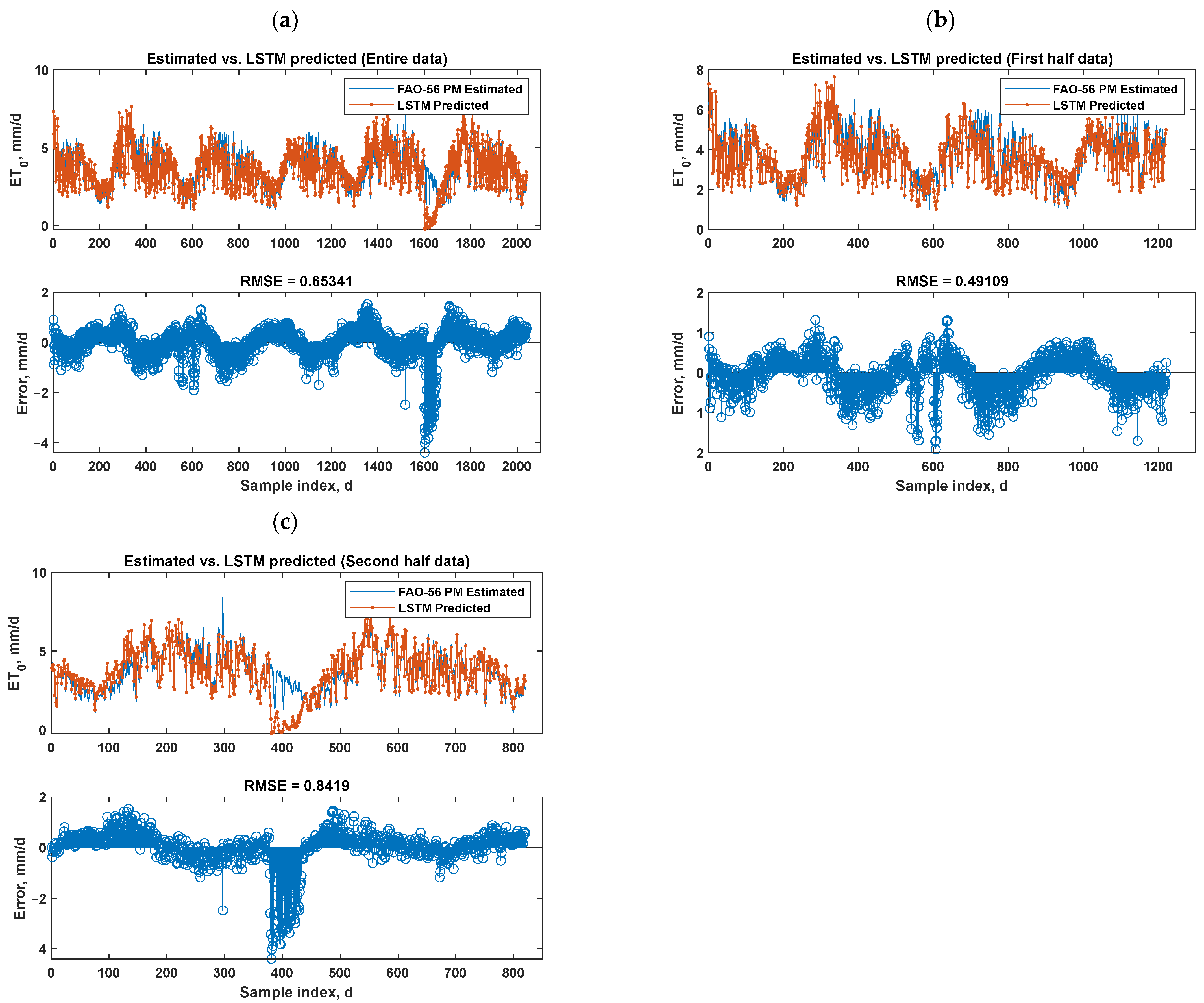
3.4.1. Generalization Capability of Proposed Best LSTM Model: Daily Prediction of ET₀

Table 13. Performance of the LSTM model for predicting daily ET₀ values on the Ishurdi dataset.

Performance Indices	Entire Dataset	First Half Data	Second Half Data
RMSE, mm/d	0.65	0.49	0.84
NRMSE	0.18	0.13	0.23
R	0.87	0.92	0.83
MAD, mm/d	0.18	0.18	0.20
MAE, mm/d	0.44	0.39	0.52
NS	0.72	0.84	0.57
IOA	0.97	0.98	0.96

summarizes the evaluation results for a variety of performance indices. The LSTM model exhibited a reasonably good performance at the test station data’s three different sets (entire, first half, and second half). The computed performance indices indicated a satisfactory performance of the proposed LSTM model. It produced reasonably higher values of benefit indices (R, NS, and IOA) and lower values of the cost indices (RMSE, NRMSE, MAD, and MAE) for the entire, the first half, and the second half of the test station data. It is also observed that the first half of the dataset produced relatively better performance when compared to that of the second half and the entire dataset. Overall, the performance is satisfactory. On this basis, it is arguably concluded that the proposed LSTM model at Gazipur Sadar station can predict daily ET₀ values at Ishurdi station without developing a model at Ishurdi station. Additionally, performance data were presented using scatter and error plots, as illustrated in Figure 11, which depict the distribution of errors at individual data points.

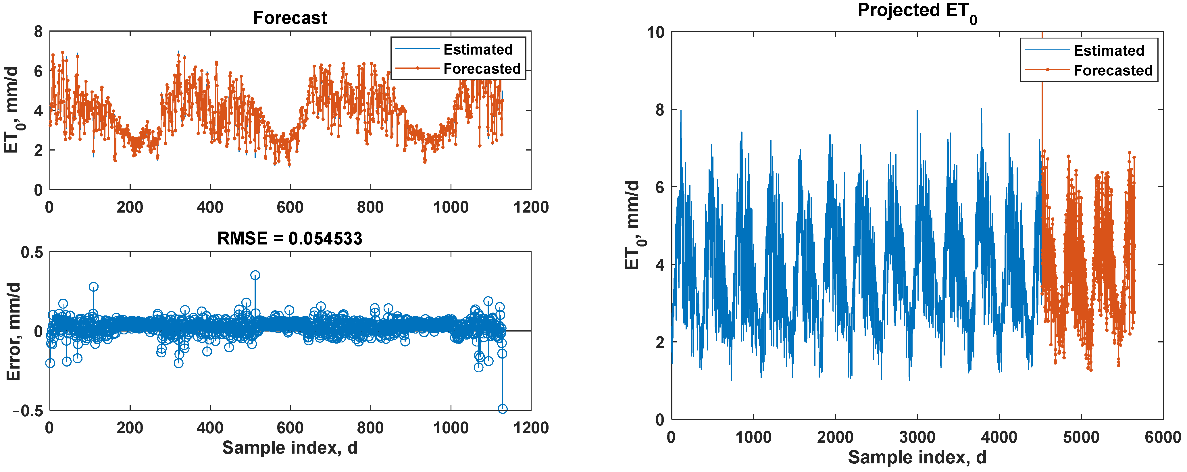
3.4.2. Generalization Capability of Proposed Best Bi-LSTM Model: Multi-Step (Multi-Day)-Ahead ET₀ Forecasting

For multi-step (multi-day)-ahead ET₀ forecasting, new Bi-LSTM models were developed because the nature of data was different. However, a similar model structure and parameters as in the case of Gazipur station were used. As a Bi-LSTM model performed better for one-step-ahead prediction at Gazipur station, the Bi-LSTM model was used to develop models for forecasting 1, 2, 3, and 5 day-ahead ET₀ values at the Ishurdi station. For this, time-lagged information from the ET₀ time series was collected for 50 lags. The most significant input variables were determined by observing partial autocorrelation functions of the lagged time series, as shown in Figure 12.

Five Bi-LSTM models were developed to forecast 1, 2, 3, 4, and 5 day-ahead ET₀ forecasting. For all models, the selected time-lagged variables were served as inputs to the Bi-LSTM models.

Table 14. Training and validation performances of the developed Bi-LSTM models at Ishurdi station.

Forecasting Horizon	Training RMSE, mm/d	Validation RMSE, mm/d
1 day	0.09	0.12
2 days	0.10	0.17
3 days	0.11	0.29
4 days	0.12	0.56
5 days	0.10	0.73

presents the performances of the proposed Bi-LSTM models at the training and validation datasets. The absolute variances between the training and validation performances increased with the increase in the forecasting horizon. Overall, the training performances were satisfactory for all forecasting horizons.

The trained and validated Bi-LSTM models were then used to forecast ET₀ values on the test dataset, which were selected from the entire dataset. Testing performances were assessed using several statistical index values, as shown in

Table 15. Multi-day-ahead forecasting performance of the Bi-LSTM model on the test dataset at Ishurdi station.

Indices	Forecasting Horizon
	1 Day	2 Days	3 Days	4 Days	5 Days
RMSE, mm/d	0.12	0.17	0.29	0.56	0.73
NRMSE	0.03	0.05	0.08	0.16	0.20
R	1.00	0.99	0.98	0.90	0.86
MAD, mm/d	0.04	0.05	0.08	0.14	0.24
MAE, mm/d	0.09	0.12	0.19	0.37	0.56
NS	0.99	0.98	0.95	0.81	0.69
IOA	1.00	1.00	0.99	0.95	0.91

. The forecasting horizon greatly influenced the forecasting accuracies. The accuracy decreased with the increase in the forecasting horizon, as in the case of the training and validation performances. However, the overall performances of the Bi-LSTM model for all forecasting horizons showed particularly good performance, as indicated by the computed statistical performance evaluation indices. Performance evaluation results of the developed models were also assessed with the aid of line graphs and error plots, as shown in Figure 13. The performance results illustrated in Figure 13 were in good agreement with the statistical index values presented in Table 15. As observed in the line graphs and error plots, forecasting accuracy largely depended on the forecasting horizon: forecasting accuracy decreased with increases in the forecasting horizon.

It is observed from Figure that 1 day- and 2 day-ahead forecasting results were relatively better when compared to the results produced in three, four, and five day-ahead forecasts with respect to the RMSE criterion. A closer look at the line graphs also revealed the superiority of one day- and two day-ahead forecasts over the other three forecasting horizons and that Bi-LSTM models captured the lower values of the ET₀ time series quite accurately in comparison with the higher values for one day-, two day-, and three day-ahead forecasts. While producing acceptable results, the Bi-LSTM models followed similar trends for both the lower and higher values in the ET₀ time series in the case of the four day- and five day-ahead forecasts. It is also perceived from the line graphs that errors were relatively smaller at the end of the time series for the one day- and two day-ahead forecasts, while the Bi-LSTM models produced relatively higher errors at the end of the dataset for the three, four, and five day-ahead forecasts. Although performed differently at different forecast horizons, the Bi-LSTM model forecasts were quite accurate and closer to the FAO-56 PM-estimated ET₀ values. This is also evident from the statistical performance evaluation indices presented in Table 15. In particular, the NRMSE values of 0.03, 0.05, 0.08, 0.16, and 0.20 for the one, two, three, four, and five day-ahead forecasts, respectively, revealed the reasonable accurate forecasts of the proposed Bi-LSTM model. A model’s performance is said to be excellent when the NRMSE value is lower than 0.1, good when the NRMSE value is between 0.1 and 0.2, fair when the NRMSE value is between 0.2 and 0.3, poor when the NRMSE is greater than 0.3 [129,130].

4. Conclusions

Precise prediction and forecasting of ET₀ have been a critical and emerging first step for developing a justifiable and effective irrigation scheduling plan. This research provided a selection of the best machine and deep learning algorithms to develop robust prediction and forecasting tools for daily and multi-step (5 day)-ahead ET₀ prediction and forecasting, respectively. The selection results indicated the superiority of the LSTM model for daily ET₀ predictions, whereas for multi-step-ahead forecasting, the Bi-LSTM model provided superior performance. For daily ET₀ prediction, a number of meteorological variables were used as inputs to the model, whereas the computed ET₀ values were used as outputs from the model. For multi-step (5 day)-ahead forecasting, the appropriate daily time-lagged ET₀ values were used as inputs to the Bi-LSTM model, and the outputs from the Bi-LSTM model were the one, two, three, four, and five step-ahead ET₀ values. On the basis of the results of the one-step-ahead prediction performed previously for model selection, we found that the Bi-LSTM model was further employed to provide multi-step (5 day)-ahead forecasting. Results revealed the suitability of the Bi-LSTM model in predicting multi-step-ahead ET₀ values.

In a further step, best models for daily prediction (LSTM) and multi-step-ahead forecasting (Bi-LSTM) were used to generalize the ET₀ values for the data obtained from a different weather station, for which the models were neither trained nor validated. More specifically, the LSTM network was used to generalize the daily ET₀ predictions in a nearby meteorological station without developing a model for that station. On the other hand, the Bi-LSTM model was developed for the Ishurdi station to forecast 1, 2, 3, 4, and 5 day-ahead ET₀ forecasting. The relatively low errors obtained by the LSTM and Bi-LSTM approaches led to a good fit of the models in predicting daily ET₀ values and forecasting multi-step-ahead ET₀ values. This can be expected to be very useful in the practice of irrigation water management, for which ET₀ is an important parameter.

References

1. Liu, S.M.; Xu, Z.W.; Zhu, Z.L.; Jia, Z.Z.; Zhu, M.J. Measurements of evapotranspiration from eddy-covariance systems and large aperture scintillometers in the Hai River Basin, China. J. Hydrol. 2013, 487, 24–38. [Google Scholar] [CrossRef]
2. Kisi, O. Modeling reference evapotranspiration using three different heuristic regression approaches. Agric. Water Manag. 2016, 169, 162–172. [Google Scholar]
3. Kool, D.; Agam, N.; Lazarovitch, N.; Heitman, J.L.; Sauer, T.J.; Ben-Gal, A. A review of approaches for evapotranspiration partitioning. Agric. For. Meteorol. 2014, 184, 56–70. [Google Scholar] [CrossRef]
4. Martí, P.; González-Altozano, P.; López-Urrea, R.; Mancha, L.A.; Shiri, J. Modeling reference evapotranspiration with calculated targets. Assessment and implications. Agric. Water Manag. 2015, 149, 81–90. [Google Scholar] [CrossRef]
5. Zhang, B.; Liu, Y.; Xu, D.; Zhao, N.; Lei, B.; Rosa, R.D.; Paredes, P.; Paço, T.A.; Pereira, L.S. The dual crop coefficient approach to estimate and partitioning evapotranspiration of the winter wheat–summer maize crop sequence in North China Plain. Irrig. Sci. 2013, 31, 1303–1316. [Google Scholar] [CrossRef]
6. Allen, R.G.; Pereira, L.S.; Raes, D.; Smith, M. Crop Evapotranspiration-Guidelines for Computing crop Water Requirements; FAO: Rome, Italy, 1998. [Google Scholar]
7. Ding, R.; Kang, S.; Zhang, Y.; Hao, X.; Tong, L.; Du, T. Partitioning evapotranspiration into soil evaporation and transpiration using a modified dual crop coefficient model in irrigated maize field with ground-mulching. Agric. Water Manag. 2013, 127, 85–96. [Google Scholar] [CrossRef]
8. Landeras, G.; Ortiz-Barredo, A.; López, J.J. Comparison of artificial neural network models and empirical and semi-empirical equations for daily reference evapotranspiration estimation in the Basque Country (Northern Spain). Agric. Water Manag. 2008, 95, 553–565. [Google Scholar] [CrossRef]
9. Ferreira, L.B.; da Cunha, F.F.; Fernandes Filho, E.I. Exploring machine learning and multi-task learning to estimate meteorological data and reference evapotranspiration across Brazil. Agric. Water Manag. 2022, 259, 107281. [Google Scholar] [CrossRef]
10. Kelley, J.; Pardyjak, E.R. Using neural networks to estimate site-specific crop evapotranspiration with low-cost sensors. Agronomy 2019, 9, 108. [Google Scholar] [CrossRef] [Green Version]
11. Yassin, M.A.; Alazba, A.A.; Mattar, M.A. Modelling daily evapotranspiration using artificial neural networks under hyper arid conditions. Pak. J. Agric. Sci. 2016, 53, 695–712. [Google Scholar]
12. Yassin, M.A.; Alazba, A.A.; Mattar, M.A. Artificial neural networks versus gene expression programming forestimating reference evapotranspiration in arid climate. Agric. Water Manag. 2016, 163, 110–124. [Google Scholar] [CrossRef]
13. Kumar, M.; Raghuwanshi, N.S.; Singh, R.; Wallender, W.W.; Pruitt, W.O. Estimating evapotranspiration using artificial neural network. J. Irrig. Drain. Eng. 2002, 128, 224–233. [Google Scholar] [CrossRef]
14. Feng, Y.; Cui, N.; Gong, D.; Zhang, Q.; Zhao, L. Evaluation of random forests and generalized regression neural networks for daily reference evapotranspiration modelling. Agric. Water Manag. 2017, 193, 163–173. [Google Scholar] [CrossRef]
15. Feng, Y.; Peng, Y.; Cui, N.; Gong, D.; Zhang, K. Modeling reference evapotranspiration using extreme learning machine and generalized regression neural network only with temperature data. Comput. Electron. Agric. 2017, 136, 71–78. [Google Scholar] [CrossRef]
16. Gocić, M.; Arab Amiri, M. Reference evapotranspiration prediction using neural networks and optimum time lags. Water Resour. Manag. 2021, 35, 1913–1926. [Google Scholar] [CrossRef]
17. Doğan, E. Reference evapotranspiration estimation using adaptive neuro-fuzzy inference systems. Irrig. Drain. 2009, 58, 617–628. [Google Scholar] [CrossRef]
18. Dou, X.; Yang, Y. Evapotranspiration estimation using four different machine learning approaches in different terrestrial ecosystems. Comput. Electron. Agric. 2018, 148, 95–106. [Google Scholar] [CrossRef]
19. Gavili, S.; Sanikhani, H.; Kisi, O.; Mahmoudi, M.H. Evaluation of several soft computing methods in monthly evapotranspiration modelling. Meteorol. Appl. 2018, 25, 128–138. [Google Scholar] [CrossRef] [Green Version]
20. Roy, D.K.; Lal, A.; Sarker, K.K.; Saha, K.K.; Datta, B. Optimization algorithms as training approaches for prediction of reference evapotranspiration using adaptive neuro fuzzy inference system. Agric. Water Manag. 2021, 255, 107003. [Google Scholar] [CrossRef]
21. Roy, D.K.; Barzegar, R.; Quilty, J.; Adamowski, J. Using ensembles of adaptive neuro-fuzzy inference system and optimization algorithms to predict reference evapotranspiration in subtropical climatic zones. J. Hydrol. 2020, 591, 125509. [Google Scholar] [CrossRef]
22. Shiri, J.; Marti, P.; Nazemi, A.H.; Sadraddini, A.A.; Kisi, O.; Landeras, G.; Fakheri Fard, A. Local vs. external training of neuro-fuzzy and neural networks models for estimating reference evapotranspiration assessed through k-fold testing. Hydrol. Res. 2013, 46, 72–88. [Google Scholar] [CrossRef]
23. Tabari, H.; Kisi, O.; Ezani, A.; Hosseinzadeh, T.P. SVM, ANFIS, regression and climate based models for reference evapotranspiration modeling using limited climatic data in a semi-arid highland environment. J. Hydrol. 2012, 444–445, 78–89. [Google Scholar] [CrossRef]
24. Huang, G.; Wu, L.; Ma, X.; Zhang, W.; Fan, J.; Yu, X.; Zeng, W.; Zhou, H. Evaluation of CatBoost method for prediction of reference evapotranspiration in humid regions. J. Hydrol. 2019, 574, 1029–1041. [Google Scholar] [CrossRef]
25. Wu, T.; Zhang, W.; Jiao, X.; Guo, W.; Alhaj Hamoud, Y. Evaluation of stacking and blending ensemble learning methods for estimating daily reference evapotranspiration. Comput. Electron. Agric. 2021, 184, 106039. [Google Scholar] [CrossRef]
26. Zhang, Y.; Zhao, Z.; Zheng, J. CatBoost: A new approach for estimating daily reference crop evapotranspiration in arid and semi-arid regions of Northern China. J. Hydrol. 2020, 588, 125087. [Google Scholar] [CrossRef]
27. Lu, X.; Fan, J.; Wu, L.; Dong, J. Forecasting multi-step ahead monthly reference evapotranspiration using hybrid extreme gradient boosting with grey wolf optimization algorithm. Comput. Model. Eng. Sci. 2020, 125, 699–723. [Google Scholar]
28. Abdullah, S.S.; Malek, M.A.; Abdullah, N.S.; Kisi, O.; Yap, K.S. Extreme Learning Machines: A new approach for prediction of reference evapotranspiration. J. Hydrol. 2015, 527, 184–195. [Google Scholar] [CrossRef]
29. Feng, Y.; Cui, N.; Zhao, L.; Hu, X.; Gong, D. Comparison of ELM, GANN, WNN and empirical models for estimating reference evapotranspiration in humid region of Southwest China. J. Hydrol. 2016, 536, 376–383. [Google Scholar] [CrossRef]
30. Wu, L.; Zhou, H.; Ma, X.; Fan, J.; Zhang, F. Daily reference evapotranspiration prediction based on hybridized extreme learning machine model with bio-inspired optimization algorithms: Application in contrasting climates of China. J. Hydrol. 2019, 577, 123960. [Google Scholar] [CrossRef]
31. Yin, Z.; Feng, Q.; Yang, L.; Deo, R.C.; Wen, X.; Si, J.; Xiao, S. Future projection with an extreme-learning machine and support vector regression of reference evapotranspiration in a mountainous inland watershed in north-west China. Water 2017, 9, 880. [Google Scholar] [CrossRef] [Green Version]
32. Ahmadi, F.; Mehdizadeh, S.; Mohammadi, B.; Pham, Q.B.; Doan, T.N.C.; Vo, N.D. Application of an artificial intelligence technique enhanced with intelligent water drops for monthly reference evapotranspiration estimation. Agric. Water Manag. 2021, 244, 106622. [Google Scholar] [CrossRef]
33. Ferreira, L.B.; da Cunha, F.F.; de Oliveira, R.A.; Fernandes Filho, E.I. Estimation of reference evapotranspiration in Brazil with limited meteorological data using ANN and SVM—A new approach. J. Hydrol. 2019, 572, 556–570. [Google Scholar] [CrossRef]
34. Torres, A.F.; Walker, W.R.; McKee, M. Forecasting daily potential evapotranspiration using machine learning and limited climatic data . Agric. Water Manag. 2011, 98, 553–562. [Google Scholar] [CrossRef]
35. Gocić, M.; Motamedi, S.; Shamshirband, S.; Petković, D.; Ch, S.; Hashim, R.; Arif, M. Soft computing approaches for forecasting reference evapotranspiration. Comput. Electron. Agric. 2015, 113, 164–173. [Google Scholar] [CrossRef]
36. Karbasi, M. Forecasting of Multi-Step Ahead Reference Evapotranspiration Using Wavelet- Gaussian Process Regression Model. Water Resour. Manag. 2018, 32, 1035–1052. [Google Scholar] [CrossRef]
37. Kisi, O.; Keshtegar, B.; Zounemat-Kermani, M.; Heddam, S.; Trung, N.T. Modeling reference evapotranspiration using a novel regression-based method: Radial basis M5 model tree. Theor. Appl. Climatol. 2021, 145, 639–659. [Google Scholar] [CrossRef]
38. Mattar, M.A. Using gene expression programming in monthly reference evapotranspiration modeling: A case study in Egypt. Agric. Water Manag. 2018, 198, 28–38. [Google Scholar] [CrossRef]
39. Mattar, M.A.; Alazba, A.A. GEP and MLR approaches for the prediction of reference evapotranspiration. Neural Comput. Appl. 2019, 31, 5843–5855. [Google Scholar] [CrossRef]
40. Alazba, A.A.; Yassin, M.A.; Mattar, M.A. Modeling daily evapotranspiration in hyper-arid environment using gene expression programming. Arab J. Geosci. 2016, 9, 202. [Google Scholar] [CrossRef]
41. Yassin, M.A.; Alazba, A.A.; Mattar, M.A. Comparison Between Gene Expression Programming and Traditional Models for Estimating Evapotranspiration under Hyper Arid Conditions. Water Resour. 2016, 43, 412–427. [Google Scholar] [CrossRef]
42. Shiri, J.; Sadraddini, A.A.; Nazemi, A.H.; Kişi, Ö.; Landeras, G.; Fakheri Fard, A.; Marti, P. Generalizability of Gene Expression Programming-based approaches for estimating daily reference evapotranspiration in coastal stations of Iran. J. Hydrol. 2014, 508, 1–11. [Google Scholar] [CrossRef]
43. Shiri, J.; Kişi, Ö.; Landeras, G.; López, J.J.; Nazemi, A.H.; Stuyt, L.C.P.M. Daily reference evapotranspiration modeling by using genetic programming approach in the Basque Country (Northern Spain). J. Hydrol. 2012, 414–415, 302–316. [Google Scholar] [CrossRef]
44. Wang, S.; Lian, J.; Peng, Y.; Hu, B.; Chen, H. Generalized reference evapotranspiration models with limited climatic data based on random forest and gene expression programming in Guangxi, China. Agric. Water Manag. 2019, 221, 220–230. [Google Scholar] [CrossRef]
45. Wang, S.; Fu, Z.-Y.; Chen, H.-S.; Nie, Y.-P.; Wang, K.L. Modeling daily reference ET in the karst area of northwest Guangxi (China) using gene expression programming (GEP) and artificial neural network (ANN). Theor. Appl. Climatol. 2016, 126, 493–504. [Google Scholar] [CrossRef]
46. Roy, D.K.; Saha, K.K.; Kamruzzaman, M.; Biswas, S.K.; Hossain, M.A. Hierarchical fuzzy systems integrated with particle swarm optimization for daily reference evapotranspiration prediction: A novel approach. Water Resour. Manag. 2021, 35, 5383–5407. [Google Scholar] [CrossRef]
47. Yan, S.; Wu, L.; Fan, J.; Zhang, F.; Zou, Y.; Wu, Y. A novel hybrid WOA-XGB model for estimating daily reference evapotranspiration using local and external meteorological data: Applications in arid and humid regions of China. Agric. Water Manag. 2021, 244, 106594. [Google Scholar] [CrossRef]
48. Başağaoğlu, H.; Chakraborty, D.; Winterle, J. Reliable evapotranspiration predictions with a probabilistic machine learning framework. Water 2021, 13, 557. [Google Scholar] [CrossRef]
49. Fu, T.; Li, X.; Jia, R.; Feng, L. A novel integrated method based on a machine learning model for estimating evapotranspiration in dryland. J. Hydrol. 2021, 603, 126881. [Google Scholar] [CrossRef]
50. Chia, M.Y.; Huang, Y.F.; Koo, C.H. Resolving data-hungry nature of machine learning reference evapotranspiration estimating models using inter-model ensembles with various data management schemes. Agric. Water Manag. 2022, 261, 107343. [Google Scholar] [CrossRef]
51. Pasqualotto, N.; D’Urso, G.; Bolognesi, S.F.; Belfiore, O.R.; Van Wittenberghe, S.; Delegido, J.; Pezzola, A.; Winschel, C.; Moreno, J. Retrieval of evapotranspiration from sentinel-2: Comparison of vegetation indices, semi-empirical models and SNAP biophysical processor approach. Agronomy 2019, 9, 663. [Google Scholar] [CrossRef] [Green Version]
52. Rodrigues, G.C.; Braga, R.P. A Simple application for computing reference evapotranspiration with various levels of data availability—ETo tool. Agronomy 2021, 11, 2203. [Google Scholar] [CrossRef]
53. Rodrigues, G.C.; Braga, R.P. Estimation of daily reference evapotranspiration from NASA POWER reanalysis products in a hot summer mediterranean climate. Agronomy 2021, 11, 2077. [Google Scholar] [CrossRef]
54. Zheng, S.; Ni, K.; Ji, L.; Zhao, C.; Chai, H.; Yi, X.; He, W.; Ruan, J. Estimation of evapotranspiration and crop coefficient of rain-fed tea plants under a subtropical climate. Agronomy 2021, 11, 2332. [Google Scholar] [CrossRef]
55. Bellido-Jiménez, J.A.; Estévez, J.; García-Marín, A.P. New machine learning approaches to improve reference evapotranspiration estimates using intra-daily temperature-based variables in a semi-arid region of Spain. Agric. Water Manag. 2021, 245, 106558. [Google Scholar] [CrossRef]
56. Vásquez, C.; Célleri, R.; Córdova, M.; Carrillo-Rojas, G. Improving reference evapotranspiration (ETo) calculation under limited data conditions in the high Tropical Andes. Agric. Water Manag. 2022, 262, 107439. [Google Scholar] [CrossRef]
57. Nourani, V.; Elkiran, G.; Abdullahi, J. Multi-step ahead modeling of reference evapotranspiration using a multi-model approach. J. Hydrol. 2020, 581, 124434. [Google Scholar] [CrossRef]
58. Tien Bui, D.; Hoang, N.-D.; Martínez-Álvarez, F.; Ngo, P.-T.T.; Hoa, P.V.; Pham, T.D.; Samui, P.; Costache, R. A novel deep learning neural network approach for predicting flash flood susceptibility: A case study at a high frequency tropical storm area. Sci. Total Environ. 2020, 701, 134413. [Google Scholar] [CrossRef]
59. Xu, H.; Zhou, J.; Asteris, P.G.; Jahed Armaghani, D.; Tahir, M.M. Supervised machine learning techniques to the prediction of tunnel boring machine penetration rate. Appl. Sci. 2019, 9, 3715. [Google Scholar] [CrossRef] [Green Version]
60. Yang, H.-F.; Chen, Y.-P.P. Hybrid deep learning and empirical mode decomposition model for time series applications. Expert Syst. Appl. 2019, 120, 128–138. [Google Scholar] [CrossRef]
61. Fang, W.; Zhong, B.; Zhao, N.; Love, P.E.D.; Luo, H.; Xue, J.; Xu, S. A deep learning-based approach for mitigating falls from height with computer vision: Convolutional neural network. Adv. Eng. Inform. 2019, 39, 170–177. [Google Scholar] [CrossRef]
62. Fan, L.; Zhang, T.; Zhao, X.; Wang, H.; Zheng, M. Deep topology network: A framework based on feedback adjustment learning rate for image classification. Adv. Eng. Inform. 2019, 42, 100935. [Google Scholar] [CrossRef]
63. Cummins, N.; Baird, A.; Schuller, B.W. Speech analysis for health: Current state-of-the-art and the increasing impact of deep learning. Methods 2018, 151, 41–54. [Google Scholar] [CrossRef] [PubMed]
64. Plappert, M.; Mandery, C.; Asfour, T. Learning a bidirectional mapping between human whole-body motion and natural language using deep recurrent neural networks. Rob. Auton. Syst. 2018, 109, 13–26. [Google Scholar] [CrossRef] [Green Version]
65. Bowes, B.D.; Sadler, J.M.; Morsy, M.M.; Behl, M.; Goodal, J.L. Forecasting groundwater table in a flood prone coastal city with long short-term memory and recurrent neural networks. Water 2019, 11, 1–38. [Google Scholar] [CrossRef] [Green Version]
66. Supreetha, B.S.; Shenoy, N.; Nayak, P. Lion algorithm-optimized long short-term memory network for groundwater level forecasting in Udupi District, India. Appl. Comput. Intell. Soft Comput. 2020, 2020, 8685724. [Google Scholar] [CrossRef] [Green Version]
67. Barzegar, R.; Aalami, M.T.; Adamowski, J. Short-term water quality variable prediction using a hybrid CNN–LSTM deep learning model. Stoch. Environ. Res. Risk Assess. 2020, 34, 415–433. [Google Scholar] [CrossRef]
68. Chang, F.-J.; Chang, L.-C.; Huang, C.-W.; Kao, I.-F. Prediction of monthly regional groundwater levels through hybrid soft-computing techniques. J. Hydrol. 2016, 541, 965–976. [Google Scholar] [CrossRef]
69. Daliakopoulos, I.N.; Coulibaly, P.; Tsanis, I.K. Groundwater level forecasting using artificial neural networks. J. Hydrol. 2005, 309, 229–240. [Google Scholar] [CrossRef]
70. Guzman, S.M.; Paz, J.O.; Tagert, M.L.M. The use of NARX neural networks to forecast daily groundwater levels. Water Resour. Manag. 2017, 31, 1591–1603. [Google Scholar] [CrossRef]
71. Bengio, Y.; Simard, P.; Frasconi, P. Learning long-term dependencies with gradient descent is difficult. IEEE Trans. Neural Netw. Learn. Syst. 1994, 5, 157–166. [Google Scholar] [CrossRef]
72. Fischer, T.; Krauss, C. Deep learning with long short-term memory networks for financial market predictions. Eur. J. Oper. Res. 2018, 270, 654–669. [Google Scholar] [CrossRef] [Green Version]
73. Zhao, Z.; Chen, W.; Wu, X.; Chen, P.C.Y.; Liu, J. LSTM network: A deep learning approach for short-term traffic forecast. IET Intell. Transp. Syst. 2017, 11, 68–75. [Google Scholar] [CrossRef] [Green Version]
74. Hu, C.; Wu, Q.; Li, H.; Jian, S.; Li, N.; Lou, Z. Deep learning with a long short-term memory networks approach for rainfall-runoff simulation. Water 2018, 10, 1543. [Google Scholar] [CrossRef] [Green Version]
75. Liang, C.; Li, H.; Lei, M.; Du, Q. Dongting lake water level forecast and its relationship with the three Gorges dam based on a long short-term memory network. Water 2018, 10, 1389. [Google Scholar] [CrossRef] [Green Version]
76. Tian, Y.; Xu, Y.-P.; Yang, Z.; Wang, G.; Zhu, Q. Integration of a parsimonious hydrological model with recurrent neural networks for improved streamflow forecasting. Water 2018, 10, 1655. [Google Scholar] [CrossRef] [Green Version]
77. Zhang, J.; Zhu, Y.; Zhang, X.; Ye, M.; Yang, J. Developing a Long Short-Term Memory (LSTM) based model for predicting water table depth in agricultural areas. J. Hydrol. 2018, 561, 918–929. [Google Scholar] [CrossRef]
78. Majhi, B.; Naidu, D.; Mishra, A.P.; Satapathy, S.C. Improved prediction of daily pan evaporation using Deep-LSTM model. Neural Comput. Appl. 2020, 32, 7823–7838. [Google Scholar] [CrossRef]
79. Hu, X.; Shi, L.; Lin, G.; Lin, L. Comparison of physical-based, data-driven and hybrid modeling approaches for evapotranspiration estimation. J. Hydrol. 2021, 601, 126592. [Google Scholar] [CrossRef]
80. Ferreira, L.B.; da Cunha, F.F. New approach to estimate daily reference evapotranspiration based on hourly temperature and relative humidity using machine learning and deep learning. Agric. Water Manag. 2020, 234, 106113. [Google Scholar] [CrossRef]
81. Roy, D.K. Long short-term memory networks to predict one-step ahead reference evapotranspiration in a subtropical climatic zone. Environ. Process. 2021, 8, 911–941. [Google Scholar] [CrossRef]
82. Ferreira, L.B.; da Cunha, F.F. Multi-step ahead forecasting of daily reference evapotranspiration using deep learning. Comput. Electron. Agric. 2020, 178, 105728. [Google Scholar] [CrossRef]
83. Ahmed, A.A.; Deo, R.C.; Feng, Q.; Ghahramani, A.; Raj, N.; Yin, Z.; Yang, L. Hybrid deep learning method for a week-ahead evapotranspiration forecasting. Stoch. Environ. Res. Risk Assess. 2021, 36, 831–849. [Google Scholar] [CrossRef]
84. Saggi, M.K.; Jain, S. Reference evapotranspiration estimation and modeling of the Punjab Northern India using deep learning. Comput. Electron. Agric. 2019, 156, 387–398. [Google Scholar] [CrossRef]
85. Granata, F.; Di Nunno, F. Forecasting evapotranspiration in different climates using ensembles of recurrent neural networks. Agric. Water Manag. 2021, 255, 107040. [Google Scholar] [CrossRef]
86. Maroufpoor, S.; Bozorg-Haddad, O.; Maroufpoor, E. Reference evapotranspiration estimating based on optimal input combination and hybrid artificial intelligent model: Hybridization of artificial neural network with grey wolf optimizer algorithm. J. Hydrol. 2020, 588, 125060. [Google Scholar] [CrossRef]
87. Yu, H.; Wen, X.; Li, B.; Yang, Z.; Wu, M.; Ma, Y. Uncertainty analysis of artificial intelligence modeling daily reference evapotranspiration in the northwest end of China. Comput. Electron. Agric. 2020, 176, 105653. [Google Scholar] [CrossRef]
88. Estévez, J.; García-Marín, A.P.; Morábito, J.A.; Cavagnaro, M. Quality assurance procedures for validating meteorological input variables of reference evapotranspiration in mendoza province (Argentina). Agric. Water Manag. 2016, 172, 96–109. [Google Scholar] [CrossRef]
89. Allen, R.G.; Pereira, L.S.; Raes, D. Evapotranspiracion ´Del Cultivo. Guías Para la Determinacion´ de Los Requerimientos de Agua de Los Cultivos (Technical Report); FAO: Roma, Italia, 2006. [Google Scholar]
90. Shiri, J.; Nazemi, A.H.; Sadraddini, A.A.; Landeras, G.; Kişi, O.; Fakheri Fard, A.; Marti, P. Comparison of heuristic and empirical approaches for estimating reference evapotranspiration from limited inputs in Iran. Comput. Electron. Agric. 2014, 108, 230–241. [Google Scholar] [CrossRef]
91. Hochreiter, S.; Schmidhuber, J. Long short-term memory. Neural Comput. 1997, 9, 1735–1780. [Google Scholar] [CrossRef]
92. Yuan, X.; Chen, C.; Lei, X.; Yuan, Y.; Muhammad Adnan, R. Monthly runoff forecasting based on LSTM–ALO model. Stoch. Environ. Res. Risk Assess. 2018, 32, 2199–2212. [Google Scholar] [CrossRef]
93. Jang, J.-S.R.; Sun, C.T.; Mizutani, E. Neuro-Fuzzy and Soft Computing: A Computational Approach to Learning and Machine Intelligence; Prentice Hall: Upper Saddle River, NJ, USA, 1997. [Google Scholar]
94. Sugeno, M.; Yasukawa, T. A fuzzy-logic-based approach to qualitative modeling. IEEE Trans. Fuzzy Syst. 1993, 1, 7. [Google Scholar] [CrossRef] [Green Version]
95. Takagi, T.; Sugeno, M. Fuzzy identification of systems and its applications to modeling and control. IEEE Trans. Syst. Man. Cybern. 1985, SMC-15, 116–132. [Google Scholar] [CrossRef]
96. Bezdek, J.C.; Ehrlich, R.; Full, W. FCM: The fuzzy c-means clustering algorithm. Comput. Geosci. 1984, 10, 191–203. [Google Scholar] [CrossRef]
97. MATLAB Version R2019b; The MathWorks, Inc.: Natick, MA, USA, 2019.
98. Jang, J.-S.R. ANFIS: Adaptive-network-based fuzzy inference system. IEEE Trans. Syst. Man. Cybern. 1993, 23, 665–685. [Google Scholar] [CrossRef]
99. Rasmussen, C.E.; Williams, C.K. Gaussian Process for Machine Learning; The MIT Press: Cambridge, MA, USA, 2006. [Google Scholar]
100. Bishop, C. Pattern Recognition and Machine Learning; Springer: New York, NY, USA, 2006. [Google Scholar]
101. Quinlan, J.R. Learning with continuous classes. In Proceedings of the Australian Joint Conference on Artificial Intelligence, Hobart, Australia, 16–18 November 1992; pp. 343–348. [Google Scholar]
102. Wang, Y.; Witten, I. Induction of model trees for predicting continuous classes. Work. Pap. 1996, 96, 23. [Google Scholar]
103. Bhattacharya, B.; Solomatine, D.P. Neural networks and M5 model trees in modelling water level–discharge relationship. Neurocomputing 2005, 63, 381–396. [Google Scholar] [CrossRef]
104. Solomatine, D.P.; Dulal, K. Model trees as an alternative to neural networks in rainfall-runoff modelling. Hydrol. Sci. J. 2003, 48, 399–411. [Google Scholar] [CrossRef]
105. Solomatine, D.P.; Yunpeng, X. M5 model trees and neural networks: Application to flood forecasting in the upper reach of the Huai River in China. J. Hydrol. Eng. 2004, 9, 491–501. [Google Scholar] [CrossRef]
106. Jekabsons, G. M5PrimeLab: M5’ Regression Tree, Model Tree, and Tree Ensemble Toolbox for Matlab/Octave; The MathWorks, Inc.: Natick, MA, USA, 2020; Available online: http://www.cs.rtu.lv/jekabsons/regression.html (accessed on 23 December 2021).
107. Friedman, J.H. Multivariate adaptive regression splines (with discussion). Ann. Stat. 1991, 19, 1–67. [Google Scholar]
108. Bera, P.; Prasher, S.O.; Patel, R.M.; Madani, A.; Lacroix, R.; Gaynor, J.D.; Tan, C.S.; Kim, S.H. Application of MARS in simulating pesticide concentrations in soil. Trans. Asabe 2006, 49, 297–307. [Google Scholar]
109. Salford-Systems. SPM Users Guide: Introducing MARS; Minitab, LLC.: State College, PA, USA, 2019; Available online: https://www.minitab.com/content/dam/www/en/uploadedfiles/content/products/spm/IntroMARS.pdf (accessed on 23 December 2021).
110. Roy, D.K.; Datta, B. Multivariate adaptive regression spline ensembles for management of multilayered coastal aquifers. J. Hydrol. Eng. 2017, 22, 4017031. [Google Scholar] [CrossRef]
111. Dempster, A.P.; Laird, N.M.; Rubin, D.B. Maximum likelihood from incomplete data via the EM algorithm. J. R. Stat. Soc. Ser. 1977, 39, 763–768. [Google Scholar]
112. MacKay, D.J.C. The evidence framework applied to classification networks. Neural Comput. 1992, 4, 720–736. [Google Scholar] [CrossRef]
113. Chen, M. Probabilistic Linear Regression. 2021. Available online: https://www.mathworks.com/matlabcentral/fileexchange/55832-probabilistic-linear-regression (accessed on 23 December 2021).
114. Yu, P.-S.; Chen, S.-T.; Chang, I.-F. Support vector regression for real-time flood stage forecasting. J. Hydrol. 2006, 328, 704–716. [Google Scholar] [CrossRef]
115. Yoon, H.; Jun, S.-C.; Hyun, Y.; Bae, G.-O.; Lee, K.-K. A comparative study of artificial neural networks and support vector machines for predicting groundwater levels in a coastal aquifer. J. Hydrol. 2011, 396, 128–138. [Google Scholar] [CrossRef]
116. Basak, D.; Pal, S.; Patranabis, D.C. Support vector regression. Neural Inf. Process. 2007, 11, 203–224. [Google Scholar]
117. Chevalier, R.F.; Hoogenboom, G.; McClendon, R.W.; Paz, J.A. Support vector regression with reduced training sets for air temperature prediction: A comparison with artificial neural networks. Neural Comput. Appl. 2011, 20, 151–159. [Google Scholar] [CrossRef]
118. Zhang, G.; Ge, H. Prediction of xylanase optimal temperature by support vector regression. Electron. J. Biotechnol. 2012, 15, 7. [Google Scholar] [CrossRef]
119. Wu, J.; Sun, J.; Liang, L.; Zha, Y. Determination of weights for ultimate cross efficiency using Shannon entropy. Expert Syst. Appl. 2011, 38, 5162–5165. [Google Scholar] [CrossRef]
120. Nash, J.E.; Sutcliffe, J.V. River flow forecasting through conceptual models part I—A discussion of principles. J. Hydrol. 1970, 10, 282–290. [Google Scholar] [CrossRef]
121. Willmot, C.J. On the validation of models. Phys. Geogr. 1981, 2, 184–194. [Google Scholar] [CrossRef]
122. Legates, D.R.; McCabe Jr, G.J. Evaluating the use of “goodness-of fit” measuresin hydrologic and hydroclimatic model validation. Water Resour. Res. 1999, 35, 233–241. [Google Scholar] [CrossRef]
123. Tao, H.; Diop, L.; Bodian, A.; Djaman, K.; Ndiaye, P.M.; Yaseen, Z.M. Reference evapotranspiration prediction using hybridized fuzzy model with firefly algorithm: Regional case study in Burkina Faso. Agric. Water Manag. 2018, 208, 140–151. [Google Scholar] [CrossRef]
124. Chia, M.Y.; Huang, Y.F.; Koo, C.H. Swarm-based optimization as stochastic training strategy for estimation of reference evapotranspiration using extreme learning machine. Agric. Water Manag. 2021, 243, 106447. [Google Scholar] [CrossRef]
125. Mohammadi, B.; Mehdizadeh, S. Modeling daily reference evapotranspiration via a novel approach based on support vector regression coupled with whale optimization algorithm. Agric. Water Manag. 2020, 237, 106145. [Google Scholar] [CrossRef]
126. Elbeltagi, A.; Deng, J.; Wang, K.; Malik, A.; Maroufpoor, S. Modeling long-term dynamics of crop evapotranspiration using deep learning in a semi-arid environment. Agric. Water Manag. 2020, 241, 106334. [Google Scholar] [CrossRef]
127. Gao, L.; Gong, D.; Cui, N.; Lv, M.; Feng, Y. Evaluation of bio-inspired optimization algorithms hybrid with artificial neural network for reference crop evapotranspiration estimation. Comput. Electron. Agric. 2021, 190, 106466. [Google Scholar] [CrossRef]
128. Yin, J.; Deng, Z.; Ines, A.V.; Wu, J.; Rasu, E. Forecast of short-term daily reference evapotranspiration under limited meteorological variables using a hybrid bi-directional long short-term memory model (Bi-LSTM). Agric. Water Manag. 2020, 242, 106386. [Google Scholar] [CrossRef]
129. Heinemann, A.B.; Oort, P.A.V.; Fernandes, D.S.; Maia, A. Sensitivity of APSIM/ORYZA model due to estimation errors in solar radiation. Bragantia 2012, 71, 572–582. [Google Scholar] [CrossRef] [Green Version]
130. Li, M.-F.; Tang, X.-P.; Wu, W.; Liu, H.-B. General models for estimating daily global solar radiation for different solar radiation zones in mainland China. Energy Convers. Manag. 2013, 70, 139–148. [Google Scholar] [CrossRef]
Figure 1. Weather station locations.
Agronomy 12 00594 g001
Figure 2. A schematic diagram of an ANFIS structure derived from a first-order Sugeno-type FIS. Reprinted with permission from Jang [98].
Agronomy 12 00594 g002
Figure 3. Absolute error boxplots. M1–M9 represent LSTM, Bi-LSTM, ANFIS, GPR, M5 tree, MARS_C, MARS_L, PLR, and SVR models, respectively.
Agronomy 12 00594 g003
Figure 4. SSR-LSTM performance: (a) estimated (FAO-56 PM-computed) and SSR-LSTM-forecasted ET0 values for the test dataset; (b) future projections beyond the observed ET0 values.
Agronomy 12 00594 g004
Figure 5. SSR-LSTM performance after network updating: (a) estimated (FAO-56 PM-computed) and SSR-LSTM-forecasted ET0 values for the test dataset; (b) future projections beyond the observed ET0 values.
Agronomy 12 00594 g005
Figure 6. ACF (a) and PACF (b) plots of the ET0 time series for 50 lags at Gazipur station.
Agronomy 12 00594 g006
Figure 7. Scatter plots and regression plots for the values of FAO-56 PM-calculated ET0 and ANFIS-forecasted ET0 for the training (a) and testing (b) phases.
Agronomy 12 00594 g007
Figure 8. FAO-56 PM-calculated and LSTM-projected ET0 values with error plots computed on the test dataset.
Agronomy 12 00594 g008
Figure 9. FAO-56 PM-calculated and Bi-LSTM-projected ET0 values with error plots computed on the test dataset.
Agronomy 12 00594 g009
Figure 10. Line graph and error plots for 1, 2, 3, 4, and 5 day-ahead forecasting at Gazipur station.
Agronomy 12 00594 g010aAgronomy 12 00594 g010b
Figure 11. Line graph and error plots of FAO-56 PM-computed and LSTM-predicted daily ET0 at Ishurdi station: (a) entire dataset, (b) first half of the dataset, and (c) second half of the dataset.
Agronomy 12 00594 g011
Figure 12. Sample partial autocorrelation functions of the lagged ET0 time series at Ishurdi station.
Agronomy 12 00594 g012
Figure 13. Line graph and error plots for 1, 2, 3, 4, and 5 day-ahead forecasting at Ishurdi station.
Agronomy 12 00594 g013