Three-Dimensional Reconstruction and Predictive Simulation Algorithm of Forest and Fruit Wood Borer Galleries Based on Two-Dimensional Images and Different Influencing Factors

Abstract

Since forest and fruit wood borer insects are very harmful, and the formed galleries are complex and not easy to observe, the 3D reconstruction and visual prediction simulation of their galleries are of great importance in agricultural and forestry research. A single image-based 3D reconstruction and visualization method is proposed. The method is divided into two steps: (1) photographing the complete insect galleries on different sample wood segments, correcting the images to obtain the complete insect tract outline, and then redefining the height of model expansion based on the distance from the outline to the midline of the outline via the sketch-based reconstruction method to reconstruct the 3D geometric model of insect tracts; (2) setting the influencing factors, such as forest and fruit wood borer pest species, host plants and insect population density, and simultaneously judging the newly added sample points and updating the original skeleton points according to the category of sample points and the comprehensive consideration of influencing factors, so as to obtain the changes of insect gallery structure under different conditions and achieve the predictive simulation of insect tract structure. We found that modeling 3D wood borer galleries by different pests on different host plants can be achieved. Compared to the hand drawing method, our method can obtain 3D models in a very short time, and the experimental models are all reconstructed within 1.5 s. The predicted variation in the range of insect tracts indicate that it was inversely proportional to the population density and positively proportional to the moth-eating ability of the pests, indicating that the method reflects the relationship between the range of insect tracts and the influencing factors. The proposed method provides a new approach to the study and control of wood borer galleries in the forest and fruit industry. In conclusion, we provide a method to reconstruct and predict the wood borer galleries in three dimensions.

1. Introduction

Forestry biological disasters caused by forestry pests are one of the major kinds of disasters threatening forestry, and their damage to forest resources and ecosystems causes substantial direct or indirect economic losses every year [1]. In the forestry and fruit industries, Saperda candida Fabricius, Carpomya vesuviana Costa, Anoplophora glabripennis, Cydia pomonella and other major, dangerous pests are responsible for invasion phenomena that are not to be underestimated [2]. Only in 2010, the economic losses caused by 16 kinds of agricultural and forestry invasive alien species, such as Aphis gossypii Glover, Agrilus mali Mats, and Leptinotarsa decemlineata (Say), amounted to 1.249 billion yuan [3]. Trunk moth larvae bore under the xylem or phloem of tree trunks, forming dense pits, destroying the phloem and transporting tissues of trees, and blocking the nutrient and water transport of host plants, leading to tree weakening or even death. In addition, because the toughness and strength of the trunk are obviously reduced after the damage, it is easily broken by the wind, which leads to safety accidents [4]. At the current stage, the control of forest and fruit wood borer insects is still based on spraying chemical pesticides or punching injections, which are more polluting to the environment, while the use of parasitic natural enemies to control moth-eating pests requires many experiments to be verified [5]. This often requires researchers to access natural parasitic enemies of the boring pest after a period of self-feeding on the experimental wood section, and then observing the activities of the boring pest and its parasitic natural enemies to obtain the effectiveness of the biological control [6]. The whole process usually takes tens of days. Since the feeding behavior of larvae is the main cause of damage to fruit trees, after understanding their feeding behavior, mastering their harmful characteristics and life patterns, establishing a three-dimensional model of their feeding channels and conducting predictive simulations can provide an effective means to improve prevention and control measures.

Simulating and predicting the movement of forest and fruit wood borer insects inside host plants is a difficult and complex task. In view of the cryptic nature of the life of forest and fruit wood borer insects, many scholars have proposed some methods to monitor them, which provide technical support to predicting the movement of pests at a later stage. Artificial sample observation [7,8] is a more commonly used monitoring method in agricultural and forestry research. The researchers dissect the affected wood segments to observe the internal structures of the insect tracts. The adult trapping technique [9,10] is based on the use of specific traps to trap adults in the experimental area, and is combined with manual observation to obtain a relevant assessment of the pests. Techniques such as remote sensing [11,12] are also used for monitoring, which are usually based on spectral features sensitive to leaf chlorophyll content that help one to achieve identification. With the advancement of computer technology and microelectronics, acoustic technology has achieved effective results in pest monitoring. This is mainly used for storage pests [13], wood quarantine pests [14,15], soil pests [16,17], and forest borer pests [18,19,20].

Currently, most research work on wood borer galleries is focused on forestry and agriculture, and the tracts are presented in 2D hand-drawn images, as they cannot be visualized in three-dimensional form. Li et al. [21] mapped the structure of the Xylotrechus rusticus L. at different damage stages by fine observation. Zhang et al. [22] obtained the damage symptoms of red-spotted white-striped aspen at different periods by visual inspection and dry dissection. Liu [23] obtained the distribution of Xylotrechus quadripes Chevrolat tracts on the trunks of affected coffee tree segments by disc analysis. Although 2D images of the galleries of wood borer pests are useful for researchers in agriculture and forestry, 2D images alone are not sufficient to study and analyze the tracts of wood borer pests because of the variety of pests and the complex structure of the tracts formed by their feeding. As the demand for virtual technology continues to rise, 3D modeling technology is receiving more and more attention and being awarded greater importance. Botanists can use numerous kinds of existing software [24,25,26] to build different plant models during their research in order to complete virtual experiments. However, most software can only simulate a limited number of existing plants, and make certain requirements of the user in terms of agricultural and forestry knowledge. Zhang et al. [27] completed a reconstruction of Agrilus subrobustus Saunders galleries using SAI scientific hand drawing as well as software such as Photoshop and Autodesk Maya. However, the above reconstruction method is not only labor-intensive and time-consuming, but also requires the user to have a clear knowledge of the damage characteristics and trunk structure of trunk-destroying pests, as well as to be familiar with the existing 3D reconstruction software.

With the development of computer technology, interdisciplinary cross-research has now become one of the hot spots of research. Its core idea is to take computer technology as the basis, and combine the disciplinary characteristics and science and technology of other disciplines to get better research results. Along with the advent and development of X-ray and MRI technologies, work on the use of computer technology for the 3D reconstruction of medical images has been carried out [28]. With 3D reconstruction technology, a model of the human organ can be constructed, and interactive manipulation of the reconstructed model can be achieved, thus enabling medical researchers to more fully understand the 3D relationship between the organ and its surrounding tissues for more accurate research and treatment purposes [29]. Meanwhile, medical image 3D reconstruction plays an important role in human simulation [30,31], virtual surgery [32], and robotic surgery [33].

In order to be able to detect the internal residual damage of plants without damaging them, many scholars have conducted some exploratory studies using non-destructive testing techniques. The instrument detection index mainly includes stress wave velocity [34], ultrasonic wave velocity [35], impedance value [36], X-ray gray value [37] and ground-penetrating radar electromagnetic ratio [38]. With the boom in computer technology, in recent years, researchers have started to experiment with a number of algorithms to achieve imaging inside wood. Du et al. [39] proposed a three-dimensional stress wave imaging method based on TKriging. Ge et al. [40] proposed a sinogram-based system rotation center to achieve high-quality CT tomography. The current NDT imaging algorithm is mainly based on laminar imaging, but it is limited by the accuracy of the sampled signal, and its capacity for reproducing the edge of the defect is not high.

However, sketch-based reconstruction is a flexible and interactive approach. Okabe et al. were [41] the first to propose the application of hand-drawn sketch modeling techniques to tree modeling and designed an interactive system to help users generate realistic tree models from sketches. Anastacio et al. [42] proposed to use a conceptual sketching approach based on construction lines to define the order of plant organs and the global structure, while locally using the L system for detail creation. Longay et al. [43] implemented a hand-drawn tree modeling system that can simulate tree growth and produce realistic tree models based on hand-drawn sketches. However, most of the aforementioned modeling focuses on the structure and characterization of plants, while simulations of the internal conditions of plants are rarely performed.

Researchers at home and abroad have conducted a lot of research on the occurrence, damage and influencing factors of forest and fruit wood borer pests. Since there are many species of moth-eating pests, such as Cerambycidae and Scolytidae in the Coleoptera family and Siricidae in Hymenoptera [44], and the morphology of the insect pathways formed by each type of pest inside the trees varies, the species of moth-eating pests can be an important factor when predicting the insect pathways. Ehrlich and Raven [45] proposed a landmark theory of synergistic evolution after studying the relationship between butterflies and their host cruciferous plants. The host plant population of the borer pest is equally diverse, and given the close relationship between the host plant and the pest, studies on the effects of different conditions of the host tree on the reproduction, survival, and damage of the borer pest are gradually being reported [46,47]. Yang [48] also compared the developmental progress and reproductive ability of Grapholita molesta Busck on six different host plants, and finally obtained the most suitable host. Thus, host plants are also an important factor influencing changes in insect population dynamics. In addition, Zhang [44] speculated, based on experimental phenomena, that when the population density on the host plant is small, the pest has a large activity space, a relatively wide moth-eating area, and a relatively long tract; while when the population density is large, the pest’s activity space and trend range are limited, so the moth-eating area is small and the tract is relatively small. Combining the results of the above studies, this paper selects pest species, host plant species, and population density as the three important influencing factors to predict the development of insect tracts.

After acquiring data on forest and fruit wood borer pest populations, most studies make scientific inferences about their development and population changes by combining their biological characteristics with the environmental conditions of the occurrence sites, and then make predictions about their occurrence trends, which mainly includes occurrence period prediction, occurrence quantity prediction, and occurrence range prediction [49]. Such predictions are mostly on the stand scale, using remote sensing image data [50,51,52] for the prediction and validation of forest pest occurrence trends over large areas. However, little work has been done to simulate the insect pathways inside monocots. It is nevertheless worthwhile to note that there exists a large body of work on the simulation and prediction of pest movement trajectories in many pests that can develop significant representational changes. For example, traditional field trials and follow-up surveys are used to study pest feeding at different times of the year [53], or manual defoliation and leaf trimming to simulate the pest [54,55,56]. However, this type of approach is time-consuming and labor-intensive, and the visualization is poor. Furthermore, with the rapid development of computerized virtual plant technology, many scholars have also used computers to simulate the dynamics of pest populations [57,58]. In addition, simulations predicting the movement and distribution patterns of insects on a single blade and the local variation of the blade also have good results. Casas et al. [59,60,61] studied and simulated the transport trajectories of insects in the plant canopy. Tang et al. [62] formed a plant functional–structural model to quantitatively simulate the effects of worm holes on single leaves of maize at different nibbling rates. All these works help us in the predictive simulation of forest and fruit wood borer galleries in this paper.

The goal of this paper is to achieve a visual predictive simulation of the spread of the forest and fruit wood borer galleries by reconstructing the tract in three dimensions from a single two-dimensional image, and incorporating changes in the influencing factors. Based on references to agricultural and forestry-related studies, the 3D reconstruction of the insect pathways was combined with the technique of sketch reconstruction. In this way, one can directly obtain a corresponding 3D model of a single wormhole by entering its 2D image and receiving a more intuitive and multi-angle view of the complete pit configuration. In addition to this approach, a simulation method for predicting insect paths based on influencing factors is proposed. The complete three-dimensional skeleton of the insect tract was used as an input sample point in connection with studies related to forest and fruit wood borer insects. By adjusting the values of three types of influencing factors, including pest species, host plants and insect population density, and the location of new insertion points, we can comprehensively determine whether the direction of pest movement within the forest stands holds true, thus enabling a visual predictive simulation of the insect path generation process.

The main contributions of this paper include the following:

(1) A contour-based 3D reconstruction method of the forest and fruit wood borer galleries is proposed. The complete contours of the forest and fruit wood borer galleries are extracted from the input single 2D images of the forest and fruit wood borer galleries, and the sketch-based reconstruction method is applied to generate 3D models. In particular, during the model’s expansion, its expansion height is determined by the distance of the corresponding contour point from the 2D contour midline, instead of the distance from the corresponding point of the contour to the ridge line used in Ref. [63];

(2) A simulation method of forest and fruit wood borer galleries prediction based on influencing factors is proposed. By extracting the 3D skeleton from the reconstructed 3D models and adding the information on 3D skeleton sample points and the changes of pest species, population density, host plants and other factors, we judge whether the new sample points conform to the movement trajectory of pests in the process of insect tract generation, thus together forming a predictive simulation of the dynamic generation of insect tracts.

2. Data Collection and Preprocessing

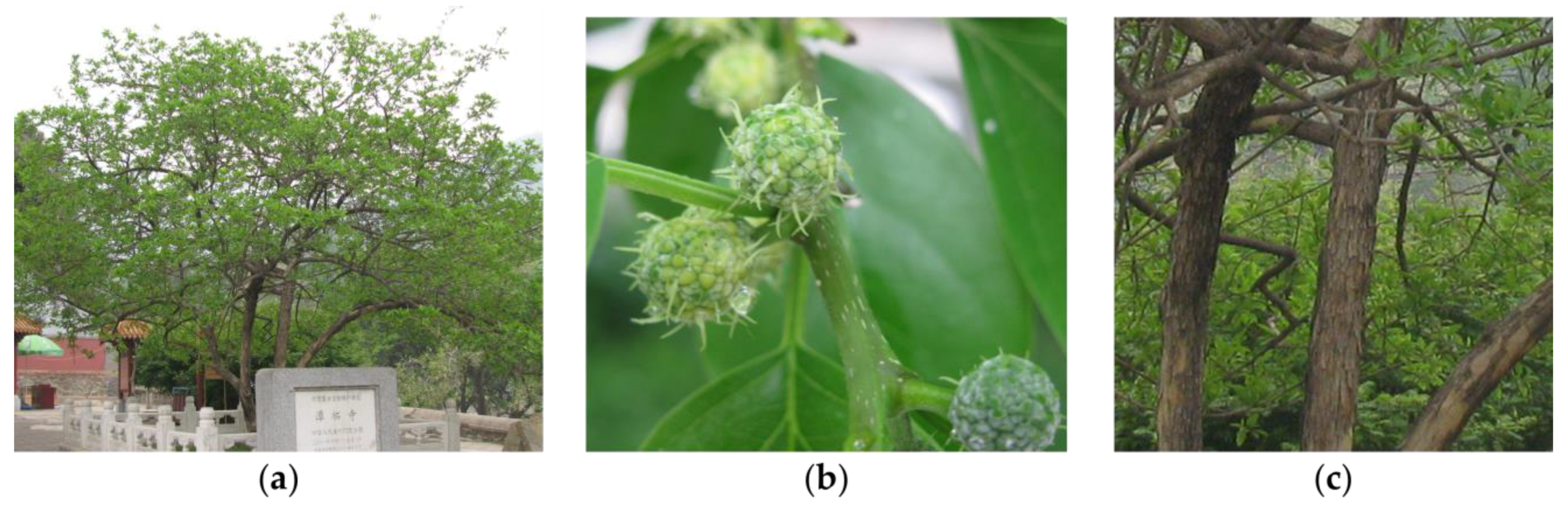
2.1. Test Data Acquisition

All the images of complete forest and fruit wood borer galleries required in this experiment were obtained by shooting. The location of the shooting was the experimental specimen room of the School of Forestry, Beijing Forestry University. We selected wood segments of specimens with high numbers of forest and fruit wood borer galleries and good structural integrity of for the study. We found the complete galleries on the infested wood section, took the complete galleries as a whole for the scene, and chose the appropriate angle to shoot from. It should be specified that in the collected images of the forest and fruit wood borer galleries, the damage sites of the host trees were located on the surfaces of the phloem and xylem, and the damage inside the xylem of the host trees was not addressed. The main species of forest and fruit wood borer were found to be cerambycidae pests. Figure 1 shows Cudrania tricuspidata; the cadres of this tree are susceptible to damage, resulting in hollow defects. The main pests and diseases on it are Apriona germar, Cicadellidae and Chrysanthemum virus B.

The camera used for the shooting was a Canon EOS 60D, and its specific parameters are shown in

Table 1. Camera parameters.

Camera Parameters	Parameter Specification
Sensor Type	CMOS
Sensor size	22.3 × 14.9 mm
Effective Pixels	18 million
Image Processor	DIGIC 4
Image resolution	Approx. 17.9 million pixels (5184 × 3456)

.

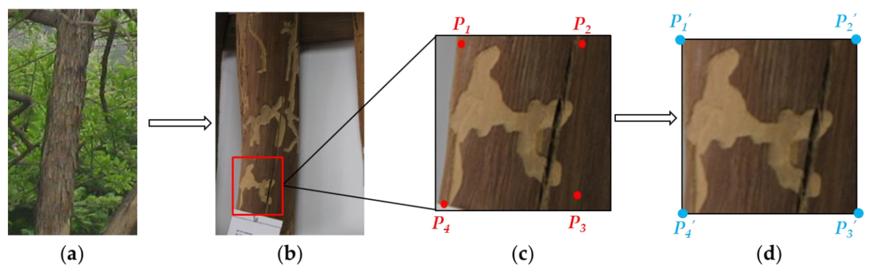
2.2. Image Correction

Since there is a certain degree of angle shift in the image acquisition process, images with deviations in their shooting angles should be corrected before the image contour extraction process. Since [H]_3×3, the transformation matrix in the projection transformation, has eight degrees of freedom, the power of the projection transformation is stronger than the other transformation forms. In this paper, a correction method based on projection transformation is used to manually select the area to be corrected and mark it. The criterion for selecting the area is that it will contain a complete worm channel in the smallest possible area. The selected area is then corrected according to the desired corrected position, and the result is shown in Figure 2.

Figure 2a shows the complete barked tree trunk; Figure 2b shows a photograph of the specimen trunk after bark removal, and we can easily see that it has more than one galleries on it, where the gallery selected by the red box is the part required for the experiment. Figure 2c shows the complete gallery selected by us, and the four sets of points (p₁–p₄) to be corrected are indicated by the red dots. Figure 2d shows the corrected image, where the green points $p_1^{\prime }$–$p_4^{\prime }$ correspond to the corrected positions of p₁–p₄ in Figure 2c, respectively.

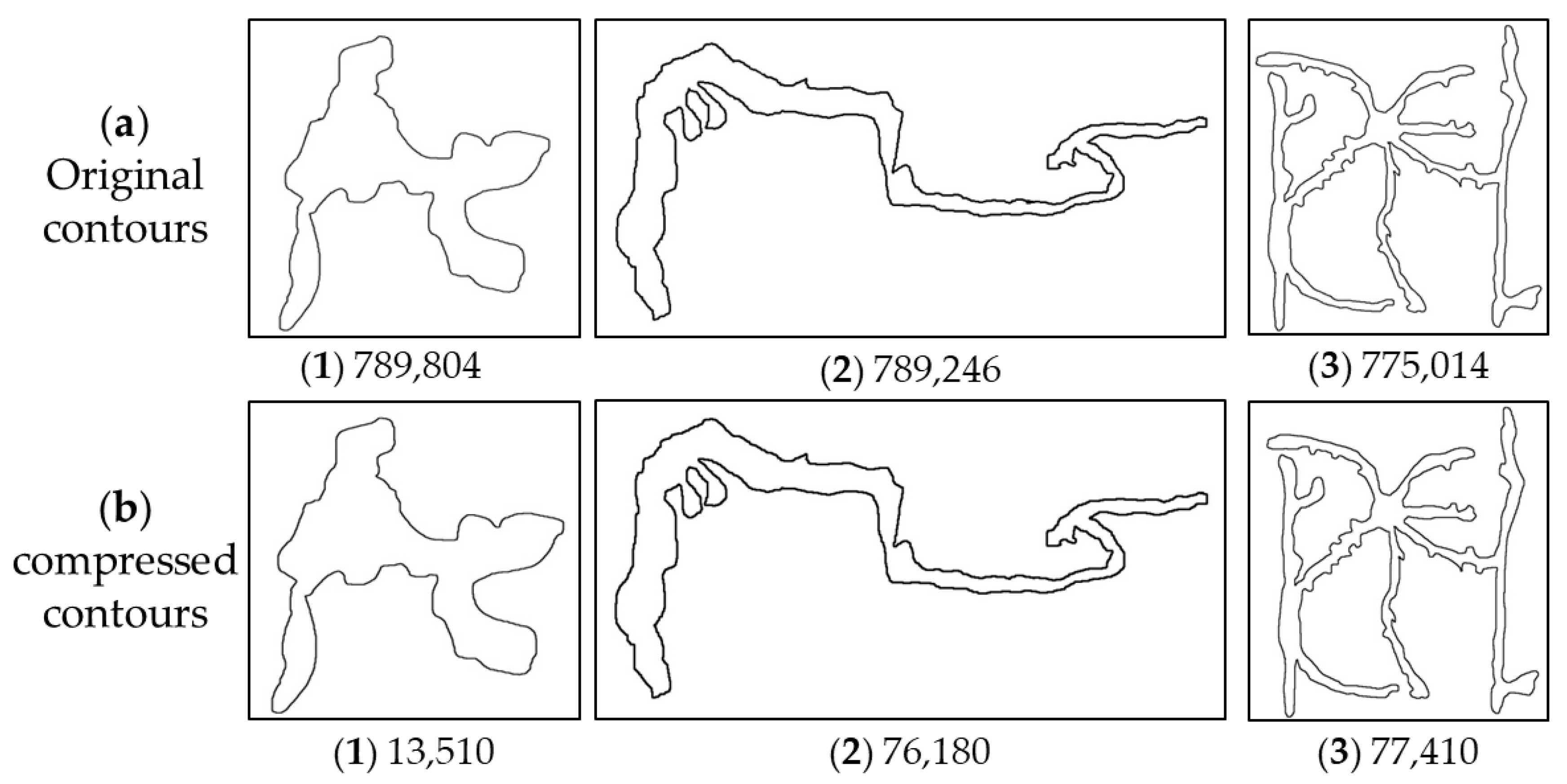
2.3. Contours Extraction and Compression

Given that there are more disturbances (e.g., cracks, holes, etc.) on the surfaces of insect-infested wood specimens due to storage time and storage environment, the results of using the automatic contour extraction method were not what we expected, so the manual method was used to extract the contours of insect paths. After manually extracting the two-dimensional contours of the forest and fruit wood borer gallery on the corrected image, the DP algorithm (Douglas–Peucker algorithm) [64] was used to compress the point set of the forest and fruit wood borer gallery contours. After compression by the DP algorithm, the overall morphology of the forest and fruit wood borer gallery contour was not changed significantly, and the detailed parts were well preserved. On the one hand, the numbers of points in the uncompressed contour point sets were relatively large, and they were partially similar, leading to many narrow triangular meshes and increasing the triangulation time when triangulation is performed. On the other hand, by compressing the contours, the numbers of contour points and similar points are reduced, resulting in a smoother surface of the resulting 3D model. The effect of compressing the contour point set using the DP algorithm is shown in Figure 3.

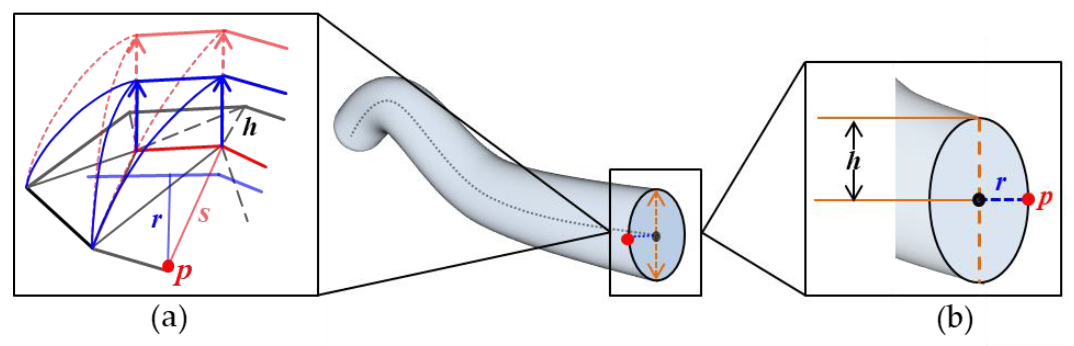
2.4. Three-Dimensional Models Reconstruction

Since the collected wood segments had all been stripped of their outer bark, resulting in the destruction of the insect tract structures on them, complete data regarding the insect tract on this wood segment could not be derived. Therefore, in the experiment, it was assumed that the collected contours were located in the centers of the original insect tracts, i.e., the insect tract structures were symmetrical on both sides of the contours. Based on the above assumptions, a sketch-based 3D reconstruction method [63] can be used to reconstruct the worm channel structure in 3D.

It is worth noting that the calculation we performed to determine the height of the ridge line elevation was different from that in the literature [63]. In this paper, the height of expansion was obtained from the distance of the point on the two-dimensional contour of the worm channel from the midline of its contour, rather than the distance of the corresponding point from the ridge line. As shown in Figure 4, we set the distance of the contour point $p$ corresponding to the ridge line from the midline $r$, and the height of the ridge lift at that point as $h$. Then, the relationship between $h$ and $r$ was determined as $h=\omega \times r$, where $h$ means the height of ridge elevation, $\omega$ means the weight value, and $r$ means the distance of the contour point from the contour midline. Since the insect path is on the curved surface of the tree trunk and there is some angular deviation during the shooting process, there remains some degree of error between the true value and the corrected value, although it has been improved. Therefore, the distance $r$ should not be directly used as the elevation height $h$ of the ridge, but a certain amount of weight should be assigned to it. The weight is larger at relatively narrow locations and smaller at relatively wide locations, i.e., $r$ is inversely proportional to $\omega$.

3. Based on Influencing Factors for Predicting Forest and Fruit Wood Borer Galleries Spread Range

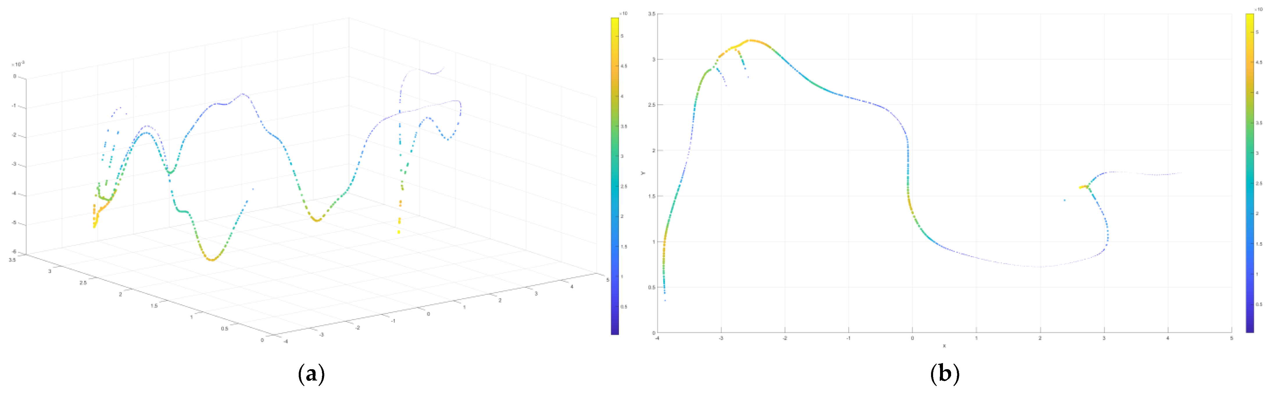
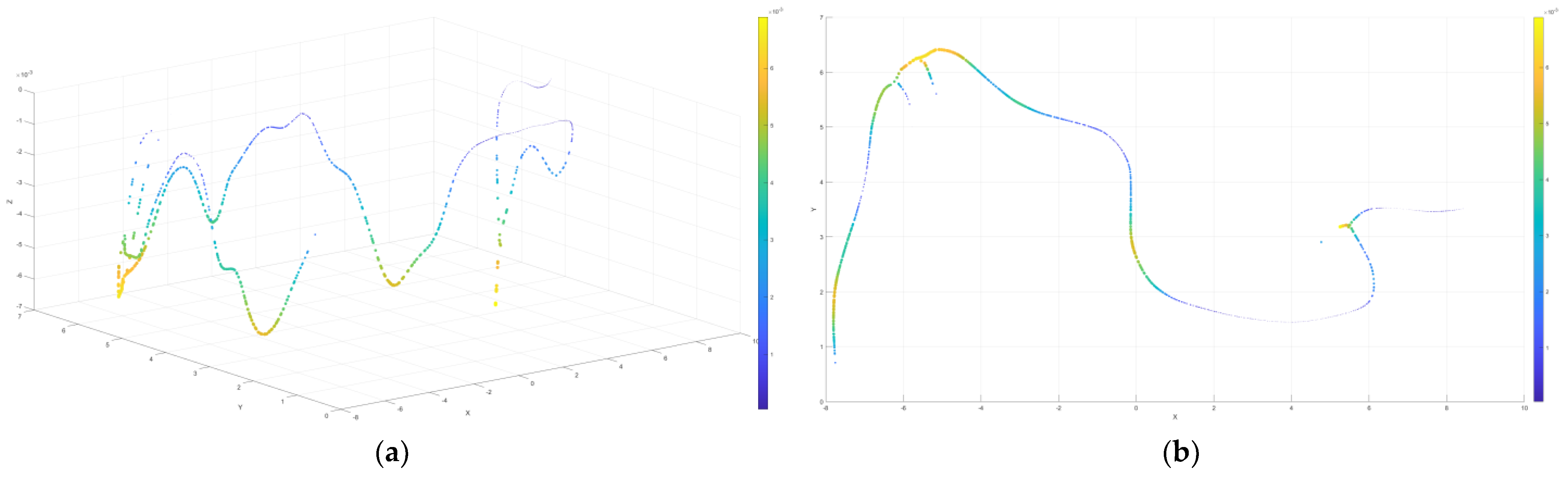
3.1. Three-Dimensional Skeleton

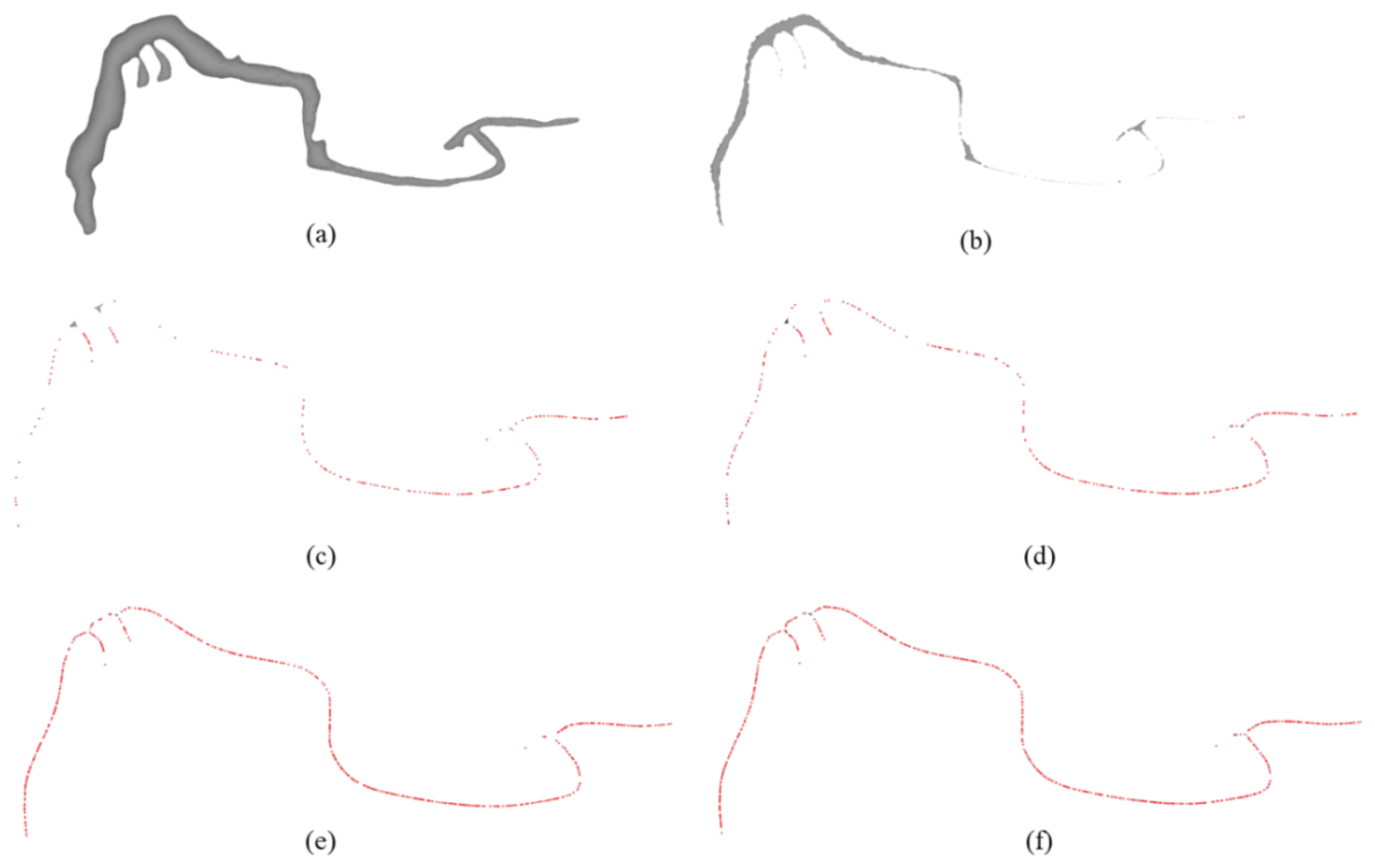
3.1.1. Three-Dimensional Skeleton Extraction

As a shape abstraction method, skeletonization has high applicability, so it is widely used in various fields. In computer graphics, the use of curved skeletons is preferred over medial skeletons, which are susceptible to complex topological disturbances. A mesh shrinkage-based curve skeleton extraction algorithm [65] was used to extract the curve skeleton from the 3D model of the forest and fruit wood borer galleries constructed in Section 2.4. This method does not require the pre-sampling of the mesh model into the volume representation, and can act directly on the mesh domain. The overall iterative process is shown in Figure 5.

3.1.2. 3D Skeleton Description

After the extraction of the 3D skeleton, we obtained a set of sample points with certain topological structures and geometric features. Therefore, we can consider the extracted skeleton as a graph G consisting of vertices V and directed edges E, as $\mathit{G}=\left(\mathit{V},\mathit{E}\right)$, where the edge $\mathit{E}$ is composed of points $v_i$ and $v_j$ with the direction $v_i$$\to$$v_j$:

$$e_{ij}=\langle v_i,v_j\rangle ,\{\begin{array}{c}{e}_{ij}\in \mathit{E}\\ v_i,v_j\in \mathit{V}\\ i,j\in \mathit{N}\end{array}$$

(1)

At the same time, each sample point $v$ has its own set of properties, as in Equation (2).

$$\mathit{A}\left(v\right)=\left(\mathit{P}\left(v\right),\mathit{F}\left(v\right),\mathit{T}\left(v\right)\right)$$

(2)

where $\mathit{A}\left(v\right)$ represents the properties of point $v$, including: $\mathit{P}\left(v\right)$ the location coordinates of the point, $\mathit{F}\left(v\right)$ the influence factor, and the time series $\mathit{T}\left(v\right)$ of the point.

Each edge also has a corresponding weight, initialized to a value of 1, which represents the number of times that edge is connected, as shown in Equation (3).

$$\mathit{W}=\sum \left(v_i,v_j\right)$$

(3)

As a side note, we will not consider the problem of the direction of the edge when calculating the number of connections between two points.

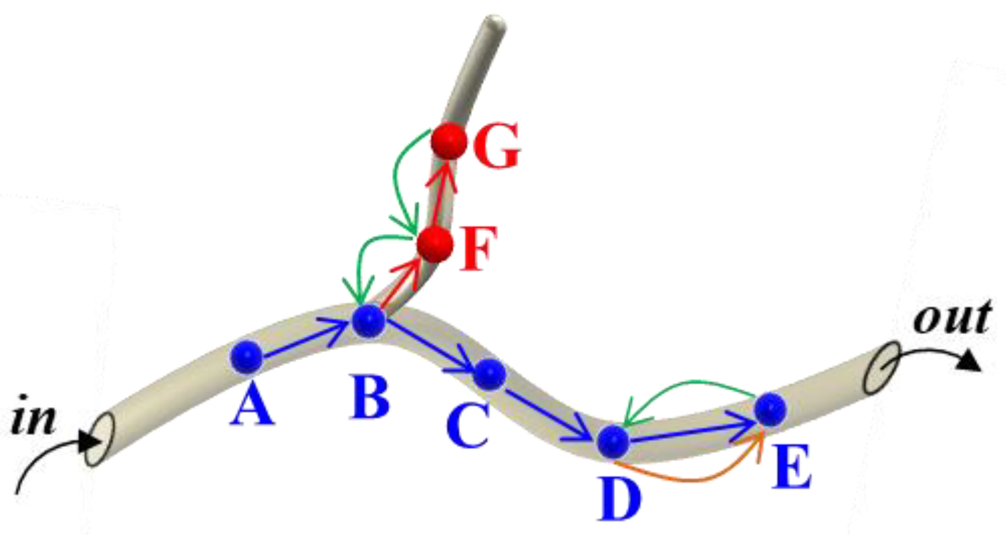
3.1.3. Description of Pest Movement

We do not have a clear picture of how the insects move inside the host plant, but based on the pictures taken and knowledge derived from research, we can make the following three classifications of their movement directions.

• Pioneering Movement

As the pest moves inside the host tree, it tends to gnaw on new branches outside the main gallery, i.e., new sample points $v$ and new points with directed edges $e$. Often, at this point, the topological ordering of the overall gallery will be different from the ordering at the previous moment. Usually, however, the overall size of the branch is smaller than the main gallery, and the pest eventually returns to the main gallery from the direction of the branch, so we call this type of movement pioneering, as shown by the red arrow in Figure 6.

2.

Forward Movement

When the pest moves inside the host tree, it moves in the direction of the main gallery towards the feathering hole, without creating a new branch outside the second. However, during the movement, the pest grows in size and may gnaw at the same location for a certain period of time, resulting in a significant increase in the size of this section of the tract. In this case, the position of the sample point at that moment remains unchanged, but the influences are updated and the weight of the side is increased. We call this type of movement forward, as shown by the blue arrow in Figure 6.

3.

Backward Movement

The same pest moves along the main insect tract as it moves inside the host, unlike the forward movement, when the pest moves in the direction of the invasion hole. As with the forward movement, the backward movement does not create new branches. Since the pest eventually needs to fly out of the plumage hole, its backward movement must produce forward movement between corresponding points after it occurs, i.e., the position of the corresponding sample point does not change, but its influencing factors are updated and the weight of the edge is increased. We call such types of motion backward motion, as shown by the green arrow in Figure 6.

3.2. Influence Factors’ Establishment

Trunk-destroying pests form galleries by feeding on the trunk of the host tree as they move inside the tree. We assume that the damage to the tree is the ratio of the volume of the insect tract to the volume of the host tree trunk:

$$E=\frac{V_{Galleries}}{V_{Tree}}$$

(4)

where $E$ is the degree of damage to the host tree, $V_{Galleries}$ denotes the volume of the insect tract, and $V_{Tree}$ denotes the volume of the host tree. Due to the relatively slow growth of the tree, it is assumed that the volume of the host tree holds a specific value during the development of the trunk moth pest from the larval to the adult stage, so it is only necessary to solve for the volume of the insect tract inside the host tree, expressed as follows:

$$V_{Galleries}=\int sdl$$

(5)

where $s$ is the maximum cross-sectional area of the insect body and $dl$ is the corresponding length. Since the pest will go through the growth process from larvae to adult inside the host tree, its body size and the area of cross-sectional surface gnawed inside the host tree will also change. Assuming that the cross-sectional area formed by the pest in the larval stage is the minimum and the cross-sectional area formed in the adult stage is the maximum, then the above volume formula can be changed to $V_{Galleries}=\int sdl,s_{min}\le s\le s_{max}$, where $s_{min}$ represents the cross-sectional area of the tract formed by larval-stage feeding and $s_{max}$ represents the cross-sectional area of the tract formed by adult-stage feeding. Since the length is determined by the speed of movement of the pest inside the host tree, $dl$ in Equation (5) can be further expressed as:

$$dl=v\times dt$$

(6)

where $v$ denotes the pest movement velocity and $dt$ denotes the movement time. Thus, the description of insect feeding inside the tree can be converted into a description of the insect size and movement speed inside the host tree, i.e., Equation (7):

$$V_{Galleries}=\int svdt,0<s_{min}\le s\le s_{max}$$

(7)

The main factors affecting the cross-sectional area and the movement speed of the pests are: pest species, host trees, population density and other external factors, which will be analyzed one by one below.

3.2.1. Forest and Fruit Wood Borer Species

Different species of pests have different body sizes, feeding sites, and movement speeds, which ultimately lead to differences in the structures of the insect tracts formed. The influence equation arising from the pest species is:

$$P=k{T}_{insect}\times jA,k,j\in (0,1)$$

(8)

where $P$ denotes the degree of influence of different species of pests, $T_{insect}$ denotes the pest species number, $A$ denotes the age of the pest, and $k$ and $j$ represent the constant coefficients.

3.2.2. Host Tree Species

In the long-term co-evolutionary process between insects and plants, the relationship between plant-feeding insects and hosts involves mutual selection, interaction and mutual adaptation, and plant-feeding insects have also formed a specific host spectrum. The probability of infestation by the same pest (preference) varies for different species of trees. Additionally, for the same species of host trees, the probability of infestation is related to the age of the tree. The influence equation for the host tree is:

$$S_{Tree}=\pi D{H}_{Tree}\times m{T}_{Tree},m\in (0,1)$$

(9)

where $S_{Tree}$ denotes the infested surface area of the host tree, $D$ denotes the diameter at breast height of the host tree, $H_{Tree}$ denotes the height of the host tree, $m$ denotes the preference of the pest for the host tree, and $T_{Tree}$ denotes the host tree species number.

3.2.3. Density of Insect Population

The population density of the sample wood segments is related to the length and diameter of the segments and the number of feathering holes on them. When the population density is small, the pest has more space to move inside the host tree, and the scope of feeding is wider, forming a relatively large insect pathway. On the contrary, when the population density is high, the space for the pest to move becomes smaller and the scope of feeding is narrower, thus forming a smaller insect pathway. The influence equation of insect population density is:

$$\rho =\frac{N_f}{\pi dL}$$

(10)

where $\rho$ denotes the population density (number of plumage holes per unit area), $N_f$ denotes the number of plumage holes on the specimen wood segment, $d$ denotes the diameter of the specimen wood segment, and $L$ denotes the length of the wood segment specimen.

3.2.4. Other Effects

In addition to the above three factors, the external environment also has an influence on the final structure of the insect tract, but since most burrowing pests live inside the host tissues and are influenced relatively little by the outside world, the influence of other external factors is expressed in this paper as $lim\epsilon \to 0^{+}$, where $\epsilon$ represents the value of other influencing factors.

In summary, combining all the influencing factors, the complete impact coefficient can be obtained as:

$$Q=aP\times b{S}_{Tree}\times c\rho +\epsilon ,\{\begin{array}{c}a>b>c\\ a,b,c\in (0,1)\end{array}$$

(11)

where $a$, $b$ and $c$ represent the constant coefficients.

The pest feeding volume inside the host tree can ultimately be expressed as $V_{Galleries}=Q\int svdt$, and the degree of damage to the host tree can be expressed as:

$$E=\frac{V_{Galleries}}{V_{Tree}}=\frac{Q\int svdt}{V_{Tree}}$$

(12)

3.3. Prediction of Forest and Fruit Wood Borer Galleries

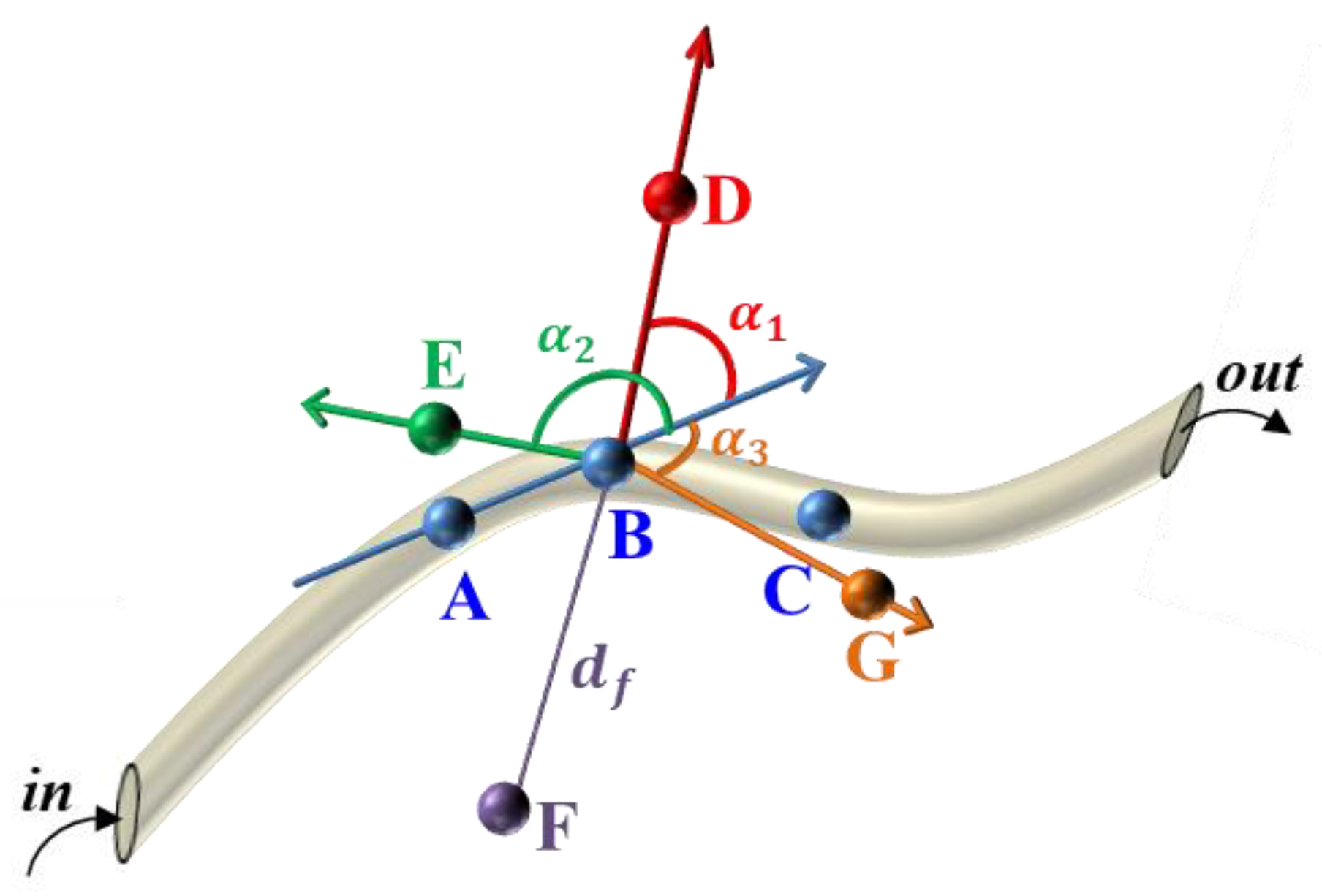
3.3.1. Define the Parameters

Before proceeding with the predictive simulation algorithm, we need to define several user-definable parameters, which are:

• The distance an insect moves per unit of time.

In this paper, we use $d_{max}$ to denote the maximum distance an insect can move per unit time within a host. The distance per unit traveled inside the host varies for each pest, due to its species and the growth period it is in. The user can control the morphological structure of the insect tract by setting different $d_{max}$ values.

2.

The angle of insect movement

In this paper, we use $\theta$ to describe the different directions of movement of the pests. Based on the three types of movement directions summarized in Section 3.1.3., we can define them in a more specific way by the range of $\theta$. Let us assume that there are three sample points $v_1$, $v_2$ and $v_3$, where $v_1$ and $v_2$ are the sample points of the previous moment and $v_3$ is the sample point of the current moment, and the corresponding two directions of motion are $\mathit{a}=\overrightarrow{v_1{v}_2}$, $\mathit{b}=\overrightarrow{v_2{v}_3}$; in this case, the angle between these two directions of motion is $\alpha$. By judging the magnitude of $\alpha$ and $\theta$, we can determine the direction of motion of the sample point $v_3$. When the absolute value of the angle between two vectors is $\left|{\alpha }_{\mathit{a}\mathit{b}}\right|\in \left[0,\theta \right]\cap \left[\pi -\theta ,\pi \right]$, this means that the movement of the pest is within the angle specified by the user, i.e., the direction of its movement is in the direction of the main gallery. When $\left|{\alpha }_{\mathit{a}\mathit{b}}\right|\in \left[\theta ,\pi -\theta \right]$, this means that the insect’s movement direction deviates from the angle set by the user, and a new branch will be created at this time.

3.

The distance of the sample point

If there are two points $\overrightarrow{v_1}$ and $\overrightarrow{v_2}$, the distance between them is calculated as:

$$d_{v_1{v}_2}=\sqrt{\left(\overrightarrow{v_1}-\overrightarrow{v_2}\right){\left(\overrightarrow{v_1}-\overrightarrow{v_2}\right)}^T}$$

(13)

4.

The angle of the sample point

Based on the definition in 2, we can calculate the angle between the two vectors as:

$${\alpha }_{\mathit{a}\mathit{b}}=arccos\frac{\left(\mathit{a}\times \mathit{b}\right)}{\left(\left|\mathit{a}\right|\times \left|\mathit{b}\right|\right)}=arccos\left(\frac{{\mathit{a}}_x{\mathit{b}}_x+{\mathit{a}}_y{\mathit{b}}_y+{\mathit{a}}_z{\mathit{b}}_z}{\left|\mathit{a}\right|\times \left|\mathit{b}\right|}\right)$$

(14)

3.3.2. Define the Prediction Point

In addition, according to the direction of motion of the insects we defined in Section 3.1.3., we can obtain three types of points corresponding to them, and one type of error point, defined as follows.

First, we assume that the current point is $v_k$, its starting point and the ending point of the previous moment are $v_{i-1}$ and $v_i$, respectively. The vectors of the two moments are $\mathit{a}=\overrightarrow{v_{i-1}{v}_i}$ and $\mathit{b}=\overrightarrow{v_i{v}_k}$.

• Pioneering Points

When the points are used to represent new branching worm paths as opposed to pioneering movements, they become pioneering points. Such points are defined as follows: ① the distance $d_{v_k{v}_i}$ from the sample point at the previous moment is less than the set distance, i.e., $d_{v_k{v}_i}\le d_{max}$; ② $\left|{\alpha }_{\mathit{a}\mathit{b}}\right|\in \left[\theta ,\pi -\theta \right]$. This is shown by the red point in Figure 7, and ${\alpha }_1={\alpha }_{\mathit{a}\mathit{b}}$.

2.

Forward Points

The point that corresponds to the forward motion and has the same position as the original sample point is called the forward point. The advancing point can be defined as follows: ① the distance $d_{v_k{v}_i}$ from the sample point at the previous moment is less than the set distance, i.e., $d_{v_k{v}_i}\le d_{max}$; ② ${\alpha }_{\mathit{a}\mathit{b}}\in \left[-\theta ,\theta \right]$. This is shown by the orange point in Figure 7, and the ${\alpha }_3={\alpha }_{\mathit{a}\mathit{b}}$.

3.

Backward Points

The backward point corresponds to the backward motion, and is used to indicate the direction of motion along the original sample point toward the intrusion hole. The backward point is defined as follows: ① the distance $d_{v_k{v}_i}$ from the sample point at the previous moment is less than the set distance, i.e., $d_{v_k{v}_i}\le d_{max}$; ② ${\alpha }_{ab}\in \left[\pi -\theta ,\pi +\theta \right]$. This is shown by the green point in Figure 7, and the ${\alpha }_2={\alpha }_{\mathit{a}\mathit{b}}$.

4.

Wrong Points

As the name implies, the error point indicates the point that the pest will not reach at the current moment. Here, the distance $d_{v_k{v}_i}$ from the sample point at the previous moment is more than the set distance, i.e., $d_{v_k{v}_i}>d_{max}$. This is shown by the purple point in Figure 7, and the $d_f=d_{v_k{v}_i}$.

3.3.3. Prediction Simulation Algorithm

Based on the parameters defined above and the types of points, we can obtain a predictive simulation algorithm for the worm path as Algorithm 1.

Algorithm 1. Simulation Algorithm for Prediction of Forest and Fruit Wood Borer Pest Galleries

Input: The three-dimensional skeleton points set $\mathit{V}$, the set of edges between the points of the three-dimensional skeleton $\mathit{E}$, the set of attributes of the points $\mathit{A}$, the set of weights of edges $\mathit{W}$, the defined movement distance $d_{max}$ and angle $\theta$, and the set of possible points $\mathit{S}$.

Output: The new 3D skeleton map ${\mathit{G}}^{\prime }$ obtained by the algorithm.

1: for i in range (0, len($\mathit{S}$)-1) do

2:  for j in range (0, len($\mathit{V}$)-1) do  3:   judge the distance between $v_j$ and $s_i$  4:   if $d_{s_i{v}_j}>d_{max}$, i = i + 1, j = 0  5:   else judge the angle $\alpha$ between $\overrightarrow{v_{j-1}{v}_j}$ and $\overrightarrow{v_j{s}_i}$  6:    if $\left|\alpha \right|\in \left[\theta ,\pi -\theta \right]$, $s_i$ insert into $\mathit{V}$, update $\mathit{V}$$,\mathit{E}$$,\mathit{A}$$,\mathit{W}$ and $\mathit{S}$

7:    else if $\alpha \in \left[-\theta ,\theta \right]$, update $v_{j+1}$ according $s_i$, update $\mathit{V}$$,\mathit{E}$$,\mathit{A}$$,\mathit{W}$ and $\mathit{S}$  8:    else update $v_{j-1}$ according to $s_i$, update $\mathit{V}$$,\mathit{E}$$,\mathit{A}$$,\mathit{W}$ and $\mathit{S}$  9:    i = 0, j = 0  10:    end if  11:  end if  12: end for  13: return the new skeleton map ${\mathit{G}}^{\prime }$

4. Result and Analysis

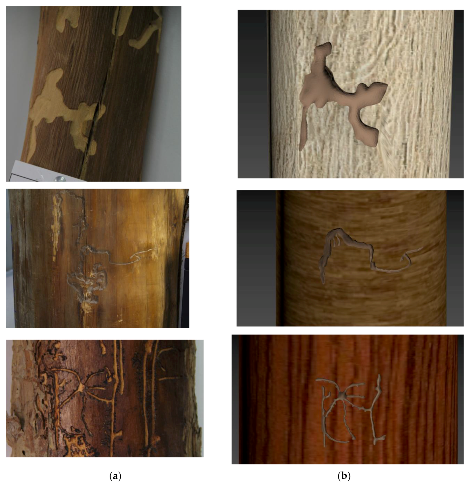
4.1. 3D Reconstruction

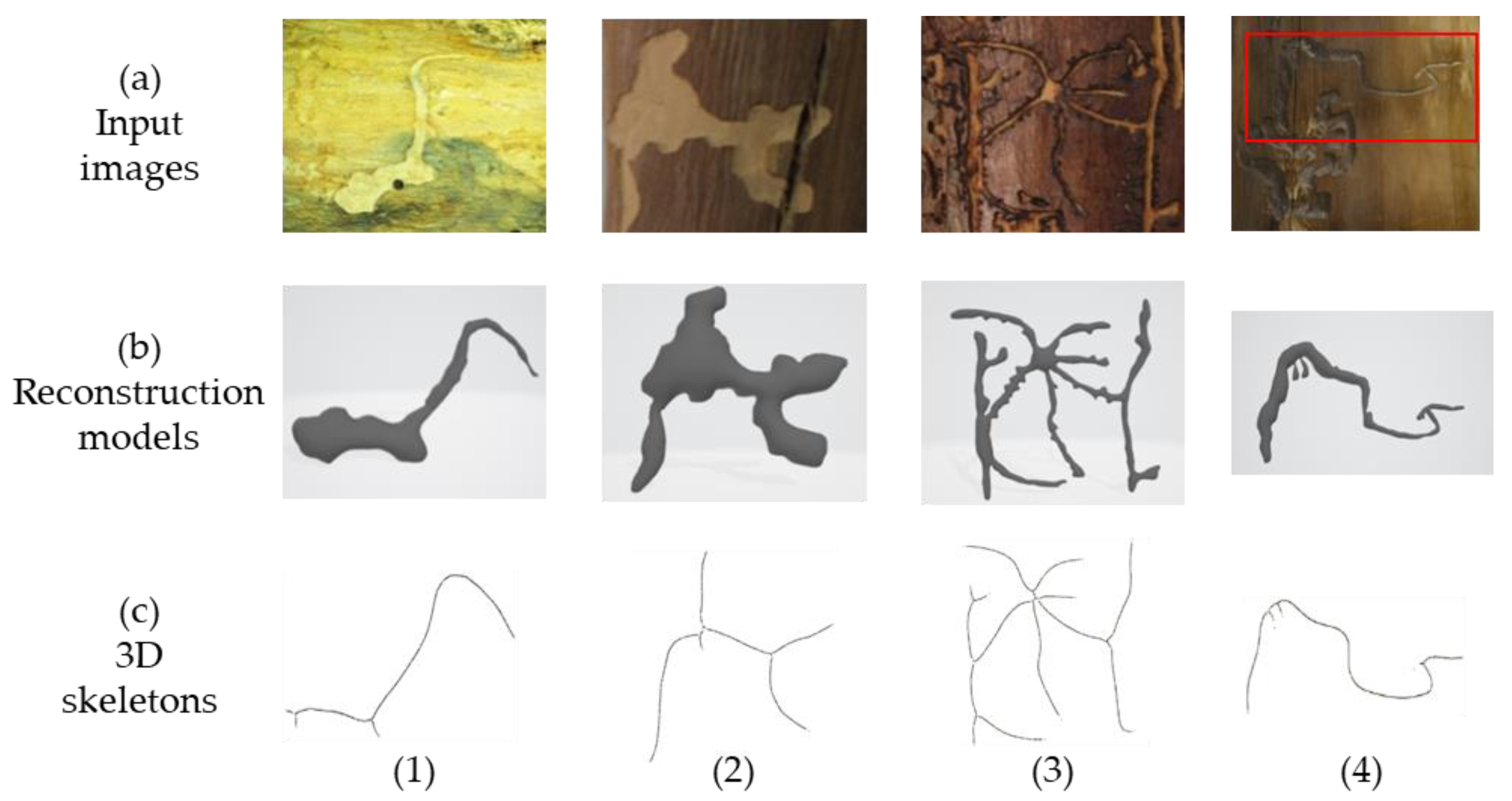
4.1.1. 3D Modeling Results of Wood Borer Galleries

The 3D model generated according to Section 2.4. and Section 3.1.1., and its corresponding 3D skeleton, are shown in Figure 8. The specific information regarding the 3D model (number of vertices and faces) and the number of points of the 3D skeleton is presented in

Table 2. Reconstruction of 3D model and 3D skeleton specific data.

Image	Species	Model	Vertexes *	Faces *	Times (s)	Skeleton Points *
Figure 8(a1)	Eucryptorrhynchus brandti	Figure 8(b1)	3812	7620	0.54	1720
Figure 8(a2)	Cerambycidae	Figure 8(b2)	6678	13,352	1.04	2074
Figure 8(a3)	Ips shangrilla	Figure 8(b3)	12,302	24,600	1.33	4644
Figure 8(a4)	Cerambycidae	Figure 8(b4)	5196	10,388	1.12	2057

* represents the number of variables.

.

The experimental results show that the contour-based 3D reconstruction algorithm proposed in this paper can be used for the 3D reconstruction of the wood borer galleries on different host plants, which are formed by different wood borer pests. The 3D model can be obtained using the contour-based 3D reconstruction algorithm. The above modeling process was conducted using the Windows 10 64-bit operating system, using the following computer configuration: Intel(R) Core(TM) i7-10700 CPU @ 2.90 GHz, 16 GB RAM. Visual Studio 2019 was used for the 3D reconstruction phase of the wood borer galleries.

4.1.2. Visualization Results

As shown in Figure 9, we have fused the 3D models of the wood borer galleries generated using the 3D reconstruction algorithm in Section 2.4. with the models of the tree trunk to achieve a visual representation of the wood borer galleries. To do this, first, we created a cylinder and selected a tree trunk mapping approach that approximates the captured image. Next, the wood borer galleries’ models obtained in Section 2.4. were combined with the tree trunks. Ultimately, a visualization of the insect galleries on the tree trunk was obtained. All the above steps were done in 3D Max 2021.

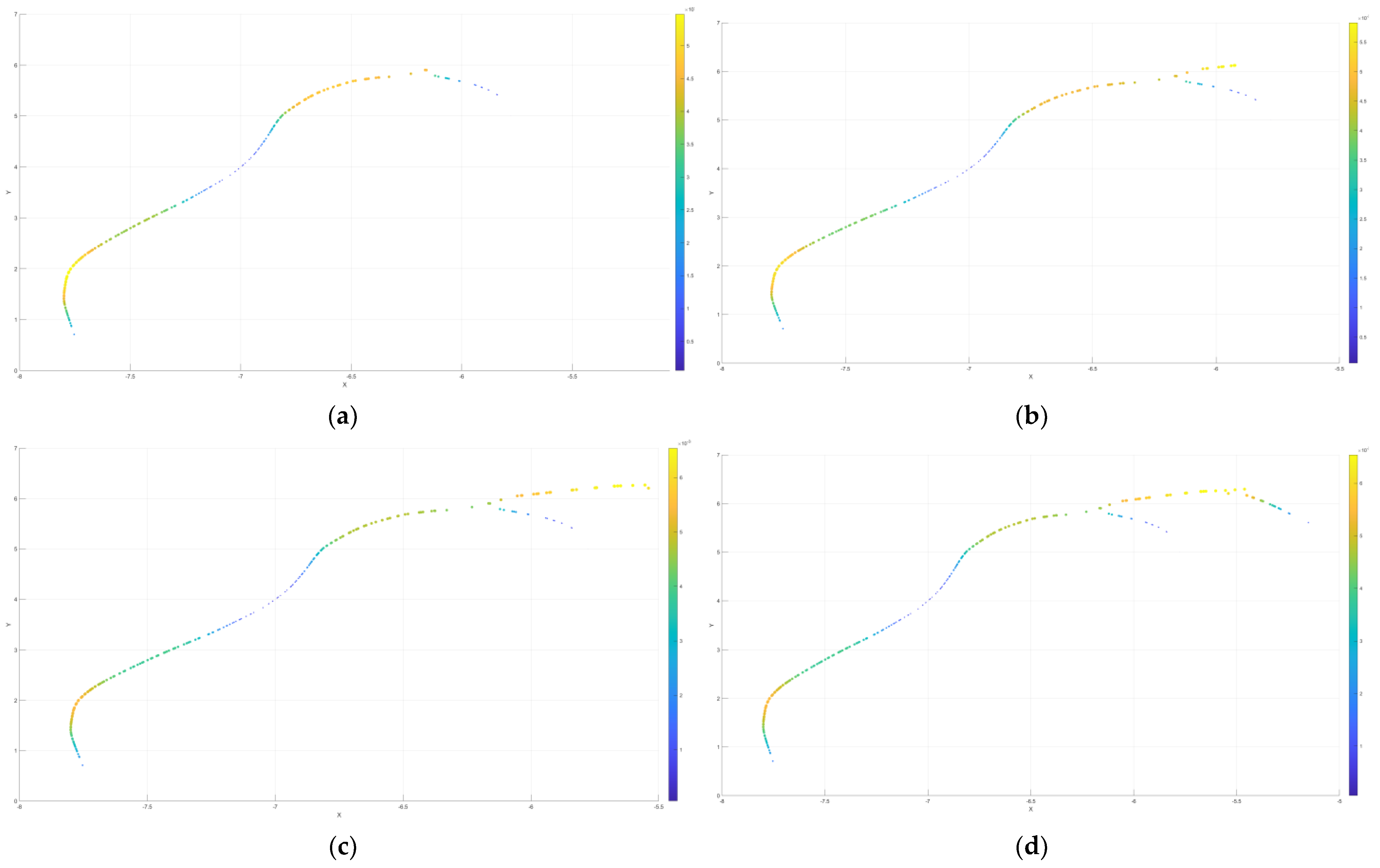
4.2. Predictive Simulation

4.2.1. Only Forward Points or Backward Points Exist

In Figure 10, a visualization of the 3D skeleton obtained from the actual sampling points is shown. It should be noted that due to the small overall thickness of the worm tract (i.e., the z-values of the sample points are small), the overall z-values of the skeleton were somewhat enlarged when we made the display in order to visualize the changes in the skeleton. Matlab 2020 was used in the visualization and presentation of the 3D skeleton.

When only forward or backward points exist, the overall structure of the worm tract is the same as that of the sampled points, i.e., the position of each sample point does not change, but the weight of each edge increases and the nature of the corresponding point changes, resulting in a change in the overall volume of the worm tract, as shown in Figure 11.

4.2.2. Only Pioneering Points Exist

We have used the branch points of the sample points for the pioneering point demonstration, as shown in Figure 12. According to the movement pattern introduced in the previous section, after traversing a new branch, the pest always returns to the main path, and continues along the direction of the main insect path before it can generate another branch.

4.2.3. Factors Influencing Regulation

According to the influencing factors mentioned in Section 3.2., changing the corresponding influencing factors will cause change in the influencing factor coefficient $Q$, such that the change in the insect tract’s structure can be simulated under different situations. In Figure 13b, the 3D skeleton information regarding the insect tract’s structure on the wood segment is based on the actual photographed samples. At this time, the influencing factors are: pest species $P=1$, host tree $S_{Tree}=2$, and population density $\rho =5$, corresponding to the influencing factor coefficient $Q=5$; if the influencing factors are adjusted to pest species $P=2$, host tree $S_{Tree}=2$, and population density $\rho =8$, the corresponding influencing factor coefficient is $Q=1$. With no change in the host tree species, the pest species changes to an insect with a relatively small borer capacity, and the density of insect mouths on the standard unit increases, resulting in a change in the overall structure of the insect tract. The extent of the insect tract is reduced and the depth of feeding is decreased, as shown in Figure 13a. If the influencing factors are adjusted to pest species $P=2$, host tree $S_{Tree}=1$, and population density $\rho =2$, then the corresponding influencing factor becomes $Q=10$. If the host tree species is changed to the species preferred by the pest, and the population density of the standard unit is decreased, the overall structure of the insect tract is changed to expand the extent of the tract and increase the depth of feeding, as shown in Figure 13c.

5. Discussion

Contour-based 3D reconstruction and predictive simulation methods have the following advantages: (1) The 3D reconstruction method of the galleries of wood borer pests [27] requires not only that the user has knowledge of agriculture and forestry, but also has some experience in using existing 3D modeling software, in addition to the time required to complete the 3D model of the insect galleries. Here, we used a contour-based reconstruction method combined with sketch reconstruction techniques [62] and redefined the height of the pest track 3D model to complete the 3D modeling of the wood borer galleries. (2) Most of the existing pest prediction simulations are focused on the stand [47] or plant surface [60]. The prediction of pests inside plants has rarely been performed. Therefore, in this paper, three factors, namely, pest species, host plant, and population density, were used to predict changes in the range of insect pathways by adjusting them, as shown in Figure 13. At the same time, three types of movements—forward, open and backward—were defined to describe the movement of the pest inside the host, thus enabling a predictive simulation of the change in the insect tract due to the movement of the pest inside the host, as shown in Figure 11 and Figure 12.

However, this approach still has some drawbacks. (1) The wood segments photographed in the experiments were all specimen wood segments. Therefore, they were pre-treated, so the structure of the wood borer galleries we observed were not complete. Also, because they were fixed and could not be moved, we could only photograph them at imperfect angles. This led us to consider solving the deformation problem due to the angle of the shot mainly in the stage of image correction. The deformation caused by camera parameters was not addressed in this paper. (2) For the height of the model mentioned in the 3D reconstruction of the wood borer galleries, the relationship between the height of the galleries and its width needs to be further demonstrated by conducting more experiments because the number of wood segments analyzed is small and the worm channels on the sample wood segments are not complete. (3) In this experiment, the collected wood borer galleries were located on the air-dried sample wood segments. However, in the real world, water content still has a greater effect on plants. The 3D reconstruction of the insect tracts on fresh host plants is not addressed in this paper. (4) Although this paper allows the work of 3D reconstruction of the insect tracts that are on the surface of the phloem and xylem, and compared to the use of chromatography [26,27], the method in this paper can obtain a 3D model with a clear outline (Figure 8b). However, for the insect tracts located inside the xylem, the method in this article do not apply. Since the insect tracts located inside the xylem cannot be contoured by a single image, therefore, the contour-based 3D reconstruction method proposed in this paper cannot be used. (5) There are still shortcomings in the algorithm design for the predictive simulation part of the wood borer gallery. The predictive simulation of insect tracts in this paper is homogeneous, i.e., every point on the tract will produce the same change under the variation of influencing factors. However, according to the related work of forestry researchers, refs. [43,44,45] there is often variation in the insect tracts eaten by wood borer pests. Therefore, to obtain more realistic predictive simulation results, the predictive simulation algorithm needs to be set up more complex and the properties of the points to be discussed need to be increased accordingly, but this will also increase the difficulty in the implementation of the algorithm.

In future work, the algorithm in this paper will be studied in more depth to obtain a more realistic reconstruction of wood borer galleries as well as predictive simulation results. Future research should be oriented in the following directions. (1) We will conduct experiments on the 3D reconstruction and visualization simulation of wood borer galleries formed by more pests in order to gain new knowledge and form better modeling methods. More experiments can also be conducted to study the differences in the effects of insect tracks formed by the same pest species in different tree species, or in the same tree species by different pests. (2) The insect tracks in the images taken in the experiments of this paper were all in dry tree trunks. Therefore, collecting new data from borer insect galleries through analysis and experiments can yield more new results, which can facilitate the more adequate design of a method for the reconstruction of insect trails, i.e., the predictive simulation algorithm.

6. Conclusions

This study presents a single image-based method for the 3D modeling of wood borer galleries. The heights of the wood borer gallery models were redefined by extracting the contours of the pest tracks using a sketch-based reconstruction method. The 3D skeleton information of the wood borer gallery was extracted using a grid-based shrinkage method. In order to predict the extents of the wood borer galleries, three types of pest movement directions, three types of influencing factors, and four types of prediction points were defined. Using this method, 3D modeling can be completed in just a few seconds. The labor and time spent in traditional modeling methods are reduced. By adjusting the influencing factors, the overall range of the worm tract’s 3D skeleton changes in proportion to changes in the influencing factors. However, the extent of the 3D skeleton of the wood borer gallery was negatively correlated with the influencing factor of the density of the pest mouths. This study overcomes the limitations of the 3D reconstruction of galleries of wood borer pests using single-image data. This method will provide a more accurate 3D model for the study and analysis of the insect galleries of wood borer pests.

References

1. Li, J.; Chang, G.B.; Qv, T.; Cui, Y.S.; Yan, J.; Song, Y.S. Hazard Assessment of Forester Pests in China. For. Pest Dis. 2019, 38, 11–17. [Google Scholar]
2. Zhu, S.J. Study on the Occurrence Characteristics of Major Pests of Forestry and Fruit Trees under Climate Change Conditions in Xinjiang Region. Master’s Thesis, Nanjing Agricultural University, Nanjing, China, 2013; p. 6. [Google Scholar]
3. Guo, W.C.; Zhang, X.L.; Wu, W.; Zhang, W.; Fu, K.Y.; Tursun, A.; Ding, X.H.; Yimit, R. Current situation, trends and research progress of invasive alien species in agriculture and foresty in oases in Xinjiang, China. J. Biosaf. 2017, 26, 1–11. [Google Scholar]
4. Zhou, M.J.; Nie, X.B.; Du, W.S.; Zhao, Y.X.; Li, J. Relationship between Sub-healthy Forest and Trunkborer-insect. J. Northeast. For. Univ. 2009, 37, 49–51. [Google Scholar]
5. Yang, L.Y.; Liu, R.J.; Zhao, X.F.; Huang, S.; Hua, J.; Sun, S.H. Vertical Distribution of Wood-boring Pests and Its Parasitic Wasp in Pinus tabulaeformis. Chin. J. Biol. Control. 2021, 34, 701–708. [Google Scholar]
6. Zhan, M.K. Studies on Population Dynamics of Woodborers and the Relationship with Pine Wilt Disease on Pinus massoniana, and Natural Enemies of Monochamus alternatus; Chinese Academy of Forestry: Beijing, China, 2014. [Google Scholar]
7. Flower, C.E.; Knight, K.S.; Gonzalez-Meler, M.A. Using stable isotopes as a tool to investigate the impacts of EAB on tree physiology and EAB spread. In Proceedings of the Emerald Ash Borer Research and Technology Development Meeting, Pittsburgh, PA, USA, 21–22 October 2009. [Google Scholar]
8. Flower, C.E.; Knight, K.S.; Rebbeck, J.; Gonzalez-Meler, M.A. The Relationship between the Emerald Ash Borer (Agrilus Planipennis) and Ash (Fraxinus spp.) Tree Decline: Using Visual Canopy Condition Assessments and Leaf Isotope Measurements to Assess Pest Damage. For. Ecol. Manag. 2013, 303, 143–147. [Google Scholar] [CrossRef]
9. Crook, D.J.; Mastro, V.C. Chemical Ecology of the Emerald Ash Borer Agrilus planipennis. J. Chem. Ecol. 2010, 36, 101–112. [Google Scholar] [CrossRef] [PubMed]
10. Mccullough, D.G.; Siegert, N.W.; Poland, T.M.; Pierce, S.J.; Ahn, S.Z. Effects of Trap Type, Placement and Ash Distribution on Emerald Ash Borer Captures in a Low Density Site. Environ. Entomol. 2011, 40, 1239–1252. [Google Scholar] [CrossRef] [Green Version]
11. Hu, B.; Li, J.; Wang, J.; Hall, B. The Early Detection of the Emerald Ash Borer (EAB) Using Advanced Geospacial Technologies. Int. Arch. Photogramm. Remote Sens. Spatial Inf. Sci. 2014, XL-2, 213–219. [Google Scholar] [CrossRef] [Green Version]
12. Zhang, K.W.; Hu, B.X.; Robinson, J. Early Detection of Emerald Ash Borer Infestation Using Multisourced Data: A Case Study in the Town of Oakville, Ontario, Canada. J. Appl. Remote Sens. 2014, 8, 083602. [Google Scholar] [CrossRef] [Green Version]
13. Li, Y.; Zhao, Z.G.; Wang, T.T.; Wu, W.Q.; Wang, X.; Ma, R.Y. Application of Sonic Signals for Fruit Damage Detection Produced by Grapholitha molesta Larval Feeding. J. Shanxi Agric. Univ. (Nat. Sci. Ed.) 2018, 38, 13. [Google Scholar]
14. Lou, D.F.; Xu, X.F.; Li, J.; Zhou, H.S.; Liu, X.J.; Li, Q.F.; Jiao, Y.; Xu, L.; Chen, D.M.; Yu, D.J.; et al. Acoustic Characteristics and Their Comparison of Six Species of Wood Borers. Plant Quar. 2013, 27, 6–10. [Google Scholar]
15. Al-Manie, M.A.; Alkanhal, M.I. Acoustic Detection of the Red Date Palm Weevil. Int. J. Electron. Commun. Eng. 2007, 1, 4. [Google Scholar]
16. Mankin, R.W.; Brandhorst-Hubbard, J.; Flanders, K.L.; Zhang, M.; Crocker, R.L.; Lapointe, S.L.; McCoy, C.W.; Fisher, J.R.; Weaver, D.K. Eavesdropping on Insects Hidden in Soil and Interior Structures of Plants. Ecol. Behav. 2000, 93, 1173–1182. [Google Scholar] [CrossRef] [PubMed] [Green Version]
17. Mankin, R.W.; Hubbard, J.L.; Flanders, K.L. Acoustic Indicators for Mapping Infestation Probabilities of Soil Invertebrates. J. Econ. Entomol. 2007, 100, 11. [Google Scholar] [CrossRef]
18. Mankin, R.W.; Mizrach, A.; Hetzroni, A.; Levsky, S.; Nakache, Y.; Soroker, V. Temporal and Spectral Features of Sounds of Wood-Boring Beetle Larvae: Identifiable Patterns of Activity Enable Improved Discrimination from Background Noise. Fla. Entomol. 2008, 91, 241–248. [Google Scholar] [CrossRef]
19. Mankin, R.W.; Smith, M.T.; Tropp, J.M.; Atkinson, E.B.; Jong, D.Y. Detection of Anoplophora glabripennis (Coleoptera: Cerambycidae) Larvae in Different Host Trees and Tissues by Automated Analyses of Sound-Impulse Frequency and Temporal Patterns. J. Econ. Entomol. 2008, 101, 12. [Google Scholar] [CrossRef]
20. Mankin, R.W.; Burman, H.; Menocal, O.; Carrillo, D. Acoustic Detection of Mallodon dasystomus (Coleoptera: Cerambycidae) in Persea Americana (Laurales: Lauraceae) Branch Stumps. Fla. Entomol. 2018, 101, 321–323. [Google Scholar] [CrossRef] [Green Version]
21. Li, W.J.; Ren, L.L.; Li, C.; Luo, Y.Q. Detailed observations on bark damage caused by the grey tiger long-horned beetle (Xylotrechus rusticus L.). Chin. J. Appl. Entomol. 2013, 50, 1270–1273. [Google Scholar]
22. Zhang, Y.K.; Long, J.M.; Zhao, C.P.; Ma, Z.L.; Zhu, G.Y.; Zhang, Z.B. Study on spatial distribution patterns of the eggs of Batocera rufomaculata and sampling techniques. China Plant Prot. 2019, 39, 25–30. [Google Scholar]
23. Liu, A.Q. Studies on Larval Tunnels and Adult Antennal Sensilla of Xylotrechus Quadripes Chevrolat. Master’s Thesis, Yunnan University, Kunming, China, 2020; p. 4. [Google Scholar]
24. Castel, T.; Beaudoin, A.; Floury, N.; Le Toan, T.; Caraglio, Y.; Barczi, J.F. Deriving forest canopy parameters for backscatter models using the AMAP architectural plant model. IEEE Trans. Geosci. Remote Sens. 2001, 39, 571–583. [Google Scholar] [CrossRef]
25. Ijiri, T.; Owada, S.; Okabe, M.; Igarashi, T. Floral Diagrams and Inflorescences: Interactive Flower Modeling Using Botanical Structural Constraints. ACM Trans. Graph. 2005, 24, 720–726. [Google Scholar] [CrossRef]
26. Lintermann, B.; Deussen, O. Interactive Modeling of Plants. IEEE Comput. Grap. Appl. 1999, 19, 56–65. [Google Scholar] [CrossRef] [Green Version]
27. Zhang, H.; Ren, L.L.; Pan, L.; Luo, Y.Q. Clarification of the species name of Agrilus subrobustus Saunders, a description of its morphological characteristics and a three-dimensional reconstruction of the larval galleries of this pest. Chin. J. Appl. Entomol. 2016, 53, 864–873. [Google Scholar]
28. Hen, N.N. 3D Reconstruction Algorithm for Medical Images. Master’s Thesis, Henan University of Technology, Zhengzhou, China, 2018; p. 5. [Google Scholar]
29. Gao, F.; Fu, Z.L. Fast marching cubes algorithm for 3D reconstruction for medical images. J. Comput. Appl. 2013, 33, 201–203, 213. [Google Scholar]
30. Pi, Y.F. Development of Computational Human Phantoms and Applications to Automated CT Image Segmentation. Ph.D. Thesis, University of Science and Technology of China, Hefei, China, 2018; p. 5. [Google Scholar]
31. Irnstorfer, N.; Unger, E.; Hojreh, A.; Homolka, P. An anthropomorphic phantom representing a prematurely born neonate for digital x-ray imaging using 3D printing: Proof of concept and comparison of image quality from different systems. Sci. Rep. 2019, 9, 14375. [Google Scholar] [CrossRef] [PubMed] [Green Version]
32. Shi, K.B. Soft Tissue Modeling Based on Medical Images and Its Application in Virtual Surgery. Master’s Thesis, Nanchang University, Nanchang, China, 2019; p. 5. [Google Scholar]
33. Zou, H.; Zhu, C.Z.; Wang, C.; Tian, G.Y.; Zhang, H.F.; Sun, C.D. Application of three-dimensional reconstruction combined with augmented reality technology in precise hepatectomy performed by robot. Chin. J. Robot. Surg. 2020, 1, 141–147. [Google Scholar]
34. Ross, R.J.; McDonald, K.A.; Green, D.W.; Schad, K.C. Relationship Between Log and Lumber Modulus of Elasticity. Wood Eng. 1997, 47, 89–92. [Google Scholar]
35. Beall, F.C. Overview of the Use of Ultrasonic Technologies in Research on Wood Properties. Wood Sci. Technol. 2002, 36, 197–212. [Google Scholar] [CrossRef]
36. Rinn, F. Intact-decay transitions in profiles of density-calibratable resistance drilling devices using long thin needles. Arboric. J. 2016, 38, 204–217. [Google Scholar] [CrossRef]
37. Ge, Z.; Chen, L.; Luo, R.; Wang, Y.; Zhou, Y. The Detection of Structure in Wood by X-ray CT Imaging Technique. BioResources 2018, 13, 3674–3685. [Google Scholar] [CrossRef]
38. Butnor, J.R.; Pruyn, M.L.; Shaw, D.C.; Harmon, M.E.; Mucciardi, A.N.; Ryan, M.G. Detecting Defects in Conifers with Ground Penetrating Radar: Applications and Challenges. For. Pathol. 2009, 39, 309–322. [Google Scholar] [CrossRef]
39. Du, X.; Feng, H.; Hu, M.; Fang, Y.; Chen, S. Three-Dimensional Stress Wave Imaging of Wood Internal Defects Using TKriging Method. Comput. Electron. Agric. 2018, 148, 63–71. [Google Scholar] [CrossRef]
40. Ge, Z.D.; Qi, Y.H.; Luo, R.; Chen, L.X.; Wang, Y.W.; Zhou, Y.C. Correction of Rotation Center for the Wood CT Imaging System. Sci. Silvae Sin. 2018, 54, 164–171. [Google Scholar]
41. Okabe, M.; Owada, S.; Igarashi, T. Interactive Design of Botanical Trees Using Freehand Sketches and Example-Based Editing. Eurographics 2005, 24, 3. [Google Scholar] [CrossRef]
42. Anastacio, F.; Prusinkiewicz, P.; Sousa, M.C. Sketch-Based Parameterization of L-Systems Using Illustration-Inspired Construction Lines and Depth Modulation. Comput. Graph. 2009, 33, 440–451. [Google Scholar] [CrossRef]
43. Longay, S.; Runions, A.; Boudon, F.; Prusinkiewicz, P. TreeSketch: Interactive Procedural Modeling of Trees on a Tablet. In Proceedings of the International Symposium on Sketch-Based Interfaces and Modeling, Annecy, France, 4–6 June 2012; pp. 107–120. [Google Scholar] [CrossRef]
44. Zhang, H. Three-Dimensional Reconstruction of the Galleries of Several Wood Borer Species. Master’s Thesis, Beijing Forestry University, Beijing, China, 2017; p. 6. [Google Scholar]
45. Ehrlich, P.R.; Raven, P.H. Butterflies and Plants: A Study in Coevolution. Evolution 1964, 18, 586–608. [Google Scholar] [CrossRef]
46. Gervais, D.J.; Green, D.F.; Work, T.T. Causes of variation in wood-boring beetle damage in fire-killed black spruce (Picea mariana) forests in the central boreal forest of Quebec. Ecoscience 2012, 19, 398–403. [Google Scholar] [CrossRef]
47. Thibault, M.; Moreau, G. Enhancing Bark- and Wood-Boring Beetle Colonization and Survival in Vertical Deadwood during Thinning Entries. J. Insect Conserv. 2016, 20, 789–796. [Google Scholar] [CrossRef]
48. Yang, X.F. Effect of Host Plant Factors on Occurrence and Growing Development and Oviposition Preference of Grapholita molesta Busck. Master’s Thesis, Hebei Agricultural University, Baoding, China, 2013; p. 6. [Google Scholar]
49. Feng, Y. Modeling, Evolution and Application of Big Data of Forest Pest in Changbai Mountains by Means of Network Science. Ph.D. Thesis, Northeastern University, Shenyang, China, 2016; p. 4. [Google Scholar]
50. Buma, B.; Pugh, E.T.; Wessman, C.A. Effect of the Current Major Insect Outbreaks on Decadal Phenological and LAI Trends in Southern Rocky Mountain Forests. Int. J. Remote Sens. 2013, 34, 7249–7274. [Google Scholar] [CrossRef]
51. Guo, Z.W.; Wu, C.Y.; Wang, X.Y. Forest insect-disease monitoring and estimation based on satellite remote sensing data. Geogr. Res. 2019, 38, 831–843. [Google Scholar]
52. Feng, L.; Jia, Z.; Li, Q.; Zhao, A.; Zhao, Y.; Zhang, Z. Spatiotemporal Change of Sparse Vegetation Coverage in Northern China. J. Indian Soc. Remote Sens. 2019, 47, 359–366. [Google Scholar] [CrossRef]
53. Cheng, Z.J.; Sun, W.; Gao, Y.B.; He, S.C.; Zhou, J.C. Damage to maize crops in Northeastern China caused by the third generation of the armyworm Mythimna separata (Walker). Chin. J. Appl. Entomol. 2018, 55, 849–856. [Google Scholar]
54. Gao, F.L.; Guo, S.M.; Yan, M.; Li, J.M.; Yu, F.H. Effects of simulated insect herbivory on the growth and chemical defense of Alternanthera philoxeroides in different habitats. Acta Ecol. Sin. 2018, 38, 2344–2352. [Google Scholar]
55. Cao, Q.J.; Yang, F.T.; Liang, Y.; Jiang, X.L.; Lamine, D.; Li, G. Simulation in Harm Degree of Mythimna seperata in Filling Stage and Its Effect on Maize Yield and Quality. Acta Agric. Boreali-Sin. 2015, 30, 180–185. [Google Scholar]
56. Schat, M.; Blossey, B. Influence of Natural and Simulated Leaf Beetle Herbivory on Biomass Allocation and Plant Architecture of Purple Loosestrife (Lythrum salicaria L.). Environ. Entomol. 2005, 34, 906–914. [Google Scholar] [CrossRef] [Green Version]
57. Su, X.Y.; Lin, C.S. Computer Simulation of Population Dynamics of the Oriental Armyworm (Mythimna separta). Acta Ecol. Sin. 1986, 6, 65–73. [Google Scholar]
58. Su, X.Y.; Lin, C.S. A Dynamic Econmic Threshold (ET) for Controlling the Oriental Armyworm (Mythimna separata W.) on Wheat. Acta Ecol. Sin. 1987, 7, 322–330. [Google Scholar]
59. Casas, J.; Aluja, M. The Geometry of Search Movements of Insects in Plant Canopies. Behav. Ecol. 1997, 8, 37–45. [Google Scholar] [CrossRef]
60. Hanan, J.; Prusinkiewicz, P.; Zalucki, M.; Skirvin, D. Simulation of Insect Movement with Respect to Plant Architecture and Morphogenesis. Comput. Electron. Agric. 2002, 35, 255–269. [Google Scholar] [CrossRef]
61. Wang, M.; Cribb, B.; Clarke, A.R.; Hanan, J. A Generic Individual-Based Spatially Explicit Model as a Novel Tool for Investigating Insect-Plant Interactions: A Case Study of the Behavioural Ecology of Frugivorous Tephritidae. PLoS ONE 2016, 11, e0151777. [Google Scholar] [CrossRef] [Green Version]
62. Tang, L.Y.; Han, W.; Lin, D.; Chen, C.C.; Chen, X.L.; Jiang, F. Visual simulation of maize growth responding to armyworm (Mythimna separata) attack. Trans. Chin. Soc. Agric. Eng. 2019, 35, 191–198. [Google Scholar]
63. Igarashi, T.; Matsuoka, S.; Tanaka, H. Teddy: A Sketching Interface for 3D Freeform Design//SIGGRAPH 07; ACM: San Diego, CA, USA, 1999. [Google Scholar] [CrossRef]
64. Douglas, D.A.; Peucker, T.K. Algorithms for the reduction of the number of points required to represent a digitized line or its caricature. Can. Cartogr. 1973, 10, 112–122. [Google Scholar] [CrossRef] [Green Version]
65. Tagliasacchi, A.; Alhashim, I.; Olson, M.; Zhang, H. Mean Curvature Skeletons. Comput. Graph. Forum 2012, 31, 1735–1744. [Google Scholar] [CrossRef] [Green Version]
Figure 1. Display of Cudrania tricuspidata: (a) the tree as a whole; (b) the fruit of the tree; (c) the trunk of the tree.
Agronomy 12 01087 g001
Figure 2. Image correction: (a) The complete trunk; (b) The trunk after bark removal; (c) The selected position points; (d) The corrected image and corresponding points.
Agronomy 12 01087 g002
Figure 3. The effect of compression using the DP algorithm: row (a) represents the original contour after manual extraction. The (a) (1) contour has 789,804 points; the (a) (2) contour has 789,246 points; and the (a) (3) contour has 775,014 points. Row (b) indicates the contours after compression using the DP algorithm. The (b) (1) contour has 13,510 points; the (b) (2) contour has 76,180 points; and the (b) (3) contour has 77,410 points.
Agronomy 12 01087 g003
Figure 4. Schematic diagram of ridge elevation. (a) shows that the expansion height defined in this paper is different from that in the literature [63]. The distance from a point p of the profile to the ridgeline is s (red), the distance to the midline of the profile is r (blue), and the height of the ridge elevation is h . (b) Schematic diagram of the transverse interface where the profile point p is located.
Agronomy 12 01087 g004
Figure 5. Three-dimensional skeleton extraction: (a) reconstructed 3D model; (b) the first iteration shrinkage; (c) the third iteration contraction; (d) the fifth iteration contraction; (e) the nth iteration contraction; (f) the three-dimensional skeleton.
Agronomy 12 01087 g005
Figure 6. The schematic diagram of pest movement directions—“in” depicts the invasion hole, and “out” the feathering hole. Blue points indicate the points on the main gallery, and red points indicate points on the branching worm paths (i.e., new points created by pioneering movements). Blue arrows indicate forward movement, red arrows indicate pioneering movement, green arrows indicate backward movement, and orange arrows indicate forward movement paired with backward movement.
Agronomy 12 01087 g006
Figure 7. The types of points. “in” denotes the invasion hole, and “out” the feathering hole. The red point indicates the pioneering point; the green point indicates backward point; the orange point indicates the forward point; the purple point indicates the wrong point.
Agronomy 12 01087 g007
Figure 8. Three-dimensional reconstruction and skeleton extraction: row (a) represents the input image; row (b) represents the 3D model generated from the 2D contour of the image in row (a); row (c) represents the 3D skeleton extracted from the 3D model in row (b).
Agronomy 12 01087 g008
Figure 9. Visualization effect display column (a) is the real shot image; column (b) is the synthetic effect.
Agronomy 12 01087 g009
Figure 10. The 3D skeleton sample point visualization display: (a) shows the skeleton sample points in 3D space; (b) shows the skeleton sample points in the x-y view. The color indicates the depth of the point, i.e., the z-value of each point. The darker the color, the shallower the depth of the point, and the brighter the color, the deeper the depth of the point.
Agronomy 12 01087 g010
Figure 11. Only forward or backward points exist. We assume an extreme case wherein the pest repeatedly performs a backwards–forwards action on the trajectory of an existing sample point, i.e., all sample points have updated attribute values. (a) shows the updated 3D view; (b) shows the updated x-y plane view. The updated worm path range changes from (−4, 5) to (−8, 10) for x, from (0, 3.5) to (0, 7) for y, and from (0.5 × 10⁻³, 5 × 10⁻³) to (1 × 10⁻³, 6 × 10⁻³) for |z|. It can be seen that the backward and forward movements have a large effect on the x and y values, while the z values change relatively little.
Agronomy 12 01087 g011
Figure 12. Only pioneering points exist. We use the branch points in the sample points to demonstrate the branch point addition process. There is only one branch in (a); (b) returns from the branch to the main worm path and continues; (c) continues in the direction of the main worm path; in (d) a second branch is generated.
Agronomy 12 01087 g012
Figure 13. Changing the influencing factors. The images in the top and bottom rows are correspondences. (a,d), (b,e) and (c,f) correspond; the first row is the 3D view and the second row is the x-y plane view. (b,e) indicates the original sampling site effect; (a,d) shows a change in pest species and population density; (c,f) shows a change in host tree species and population density.
Agronomy 12 01087 g013