Segmentation of Individual Leaves of Field Grown Sugar Beet Plant Based on 3D Point Cloud

Abstract

Accurate segmentation of individual leaves of sugar beet plants is of great significance for obtaining the leaf-related phenotypic data. This paper developed a method to segment the point clouds of sugar beet plants to obtain high-quality segmentation results of individual leaves. Firstly, we used the SFM algorithm to reconstruct the 3D point clouds from multi-view 2D images and obtained the sugar beet plant point clouds after preprocessing. We then segmented them using the multiscale tensor voting method (MSTVM)-based region-growing algorithm, resulting in independent leaves and overlapping leaves. Finally, we used the surface boundary filter (SBF) method to segment overlapping leaves and obtained all leaves of the whole plant. Segmentation results of plants with different complexities of leaf arrangement were evaluated using the manually segmented leaf point clouds as benchmarks. Our results suggested that the proposed method can effectively segment the 3D point cloud of individual leaves for field grown sugar beet plants. The leaf length and leaf area of the segmented leaf point clouds were calculated and compared with observations. The calculated leaf length and leaf area were highly correlated with the observations with R² (0.80–0.82). It was concluded that the MSTVM-based region-growing algorithm combined with SBF can be used as a basic segmentation step for high-throughput plant phenotypic data extraction of field sugar beet plants.

1. Introduction

Sugar beet is the second most important sugar crop after sugar cane [1] and supplies approximately 35% of the sugar in the world [2]. The phenotypic and genotypic data are the key elements for sugar beet breeding [3]. The acquisition of sugar beet genotypic data has been largely resolved through the development of the high-throughput DNA sequencing technology [4]. In 2004, Dohm et al. presented a reference genome sequence for sugar beet for the first time [5]. However, the data required for phenotyping still rely on manual measurements, which are time-consuming and expensive [6]. Segmenting individual leaves of individual plants in field canopies of sugar beet is meaningful for acquisition of the phenotype information of field grown sugar beet plants, it would be very helpful to better calculate the information of individual organs of sugar beet breeding materials, such as leaf length, leaf area, leaf spatial layout, and light interception at different angles of single leaf, etc. The phenotypic information would be a benefit for selecting breeding varieties. The lack of efficient and accurate methods of data acquisition of sugar beet phenotyping has become a bottleneck restricting sugar beet breeding [7].

The leaf is the main photosynthetic organ of plants and its shape largely affects photosynthesis and determines the yield [8]. Although there are currently many leaf segmentation methods based on two-dimensional (2D) images [9,10], it is very challenging to obtain steric information of leaves accurately [11]. Nowadays, many studies have demonstrated that the analysis of three-dimensional (3D) plants would provide more accurate results in segmentation and phenotypic data extraction [12,13]. Three-dimensional reconstruction techniques can be divided into two main categories: active illumination-based approaches and passive approaches [14]. Active illumination approaches use sensors to emit lights and do not depend on external light, such as Light Detection and Ranging (LiDAR) [15] and time of flight (TOF) [16]. Jin et al. [17] proposed a median normalized-vector growth (MNVG) algorithm to segment the maize point clouds obtained by LiDAR and found that the mean accuracy of segmentation at point level in terms of the F-score was 0.92 and the accuracy of phenotypic trait extraction was more than 0.96. Bao et al. [16] and Xiang et al. [18] used the Kinect to obtain maize point cloud in the field and sorghum point cloud in the laboratory. Both studies obtained the skeleton of the plants after slicing before applying clustering methods to classify the leaves and stems of plants. The extracted phenotypic data verified the effectiveness of the segmentation methods. Harmening et al. [19] proposed a fully automatic leaf segmentation method to segment the time series 3D point clouds of cucumber plants acquired by an automotive grade laser scanner. It revealed the consistency with maximal deviations in the determined leaf areas up to 5%.

In the passive approach, multi-view images are used to reconstruct 3D canopies. The structure from motion (SFM), one of the passive approaches that have been widely used, is a simple, easy-to-use, and robust passive method [20,21]. Ghahremani et al. [22] used the random sample consensus (RANSAC) to analyze both Brassica and grapevine 3D point clouds and found that the predicted leaf angle and branch angle were highly correlated with the measured values (R² > 0.90). Elnashef et al. [23] proposed a tensor-based 3D plant model segmentation algorithm to divide the point cloud into leaves and stems for wheat, maize, and cotton seedlings grown in laboratory. Miao et al. [24] applied the Laplacian based method to 3D point cloud of the field grown maize in order to obtain the skeleton and to classify the leaves and stems. This method could also be used to segment newly grown leaves. Liu et al. [25] proposed an automated selection method based on support vector machine (SVM) algorithm to classify the stems and leaves of the potted plant point cloud. The characteristic of this SVM based method is that the running speed is relatively fast, but the processing capacity for overlapping leaves is limited. Gélard et al. [26] used a plant model-based segmentation method to separate the point clouds of sunflower and sorghum plants. Shi et al. [27] used a fully convolutional network (FCN) and a masked region-based convolutional neural network (R-CNN) to perform semantic and instance segmentation on the 2D images and combined all the 2D predicted segmentations to segment the 3D point cloud with satisfactory results. Liu et al. [28] proposed a method based on existing Euclidean distance and spectral clustering algorithms to segment the Brassica point cloud and found that their approach could effectively segment the obtained point clouds. These segmentation approaches can work on point clouds from either the active approaches or passive approaches.

In addition to SFM method, stereo vision is another reliable way to collect point clouds [29]. By combining depth information, a point cloud can be obtained by restoring pixels in a 2D image to 3D space. Müller-Linow et al. [30] tested stereo imaging on sugar beet plants and developed a software package which was also used by Pinto et al. [31]. This package combines depth and color information to segment green leaf material. Scholz et al. [32] used three cameras as two camera pairs to generate depth information, while individual plant components of the beet plant were manually segmented.

Due to the complexity of the 3D structural data of field grown sugar beet, an accurate leaf segmentation is a challenge, and the existing methods do not meet the requirements yet. The goal of this study was to propose a method to segment the 3D point cloud of sugar beet plants to obtain individual leaves, in view of the complex leaf layout of the 3D data acquired in the field. This study first obtained point clouds of sugar beet plants reconstructed by the SFM method and manually removed the background points. Then, we proposed a combined method to segment the point cloud of field grown sugar beet plants, where the performance of the method was compared on sugar beet plants with different complexities. Finally, to evaluate the availability of the point cloud segmentation results, we extracted leaf length and leaf area from individual leaf point clouds.

2. Materials and Methods

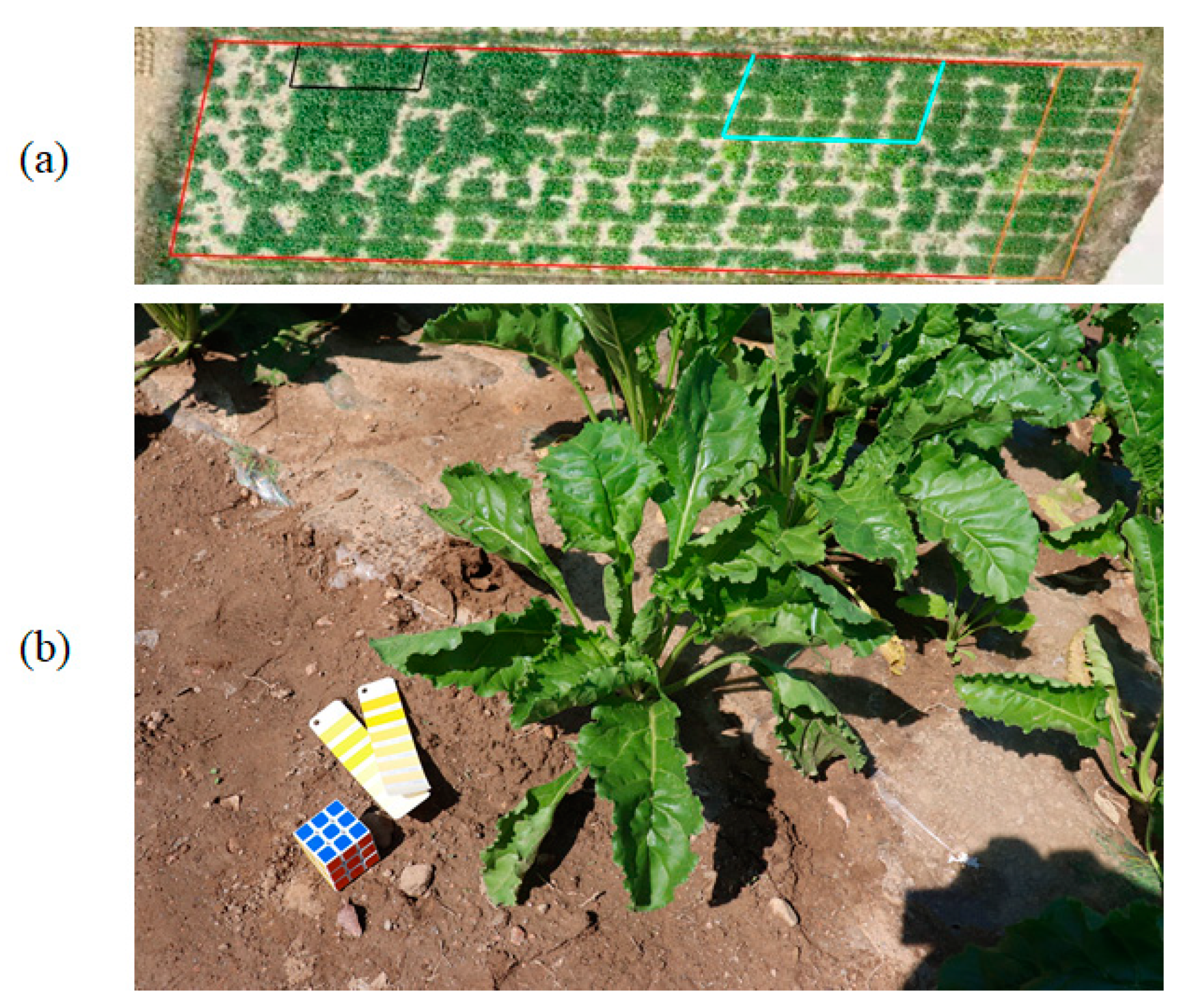
2.1. Field Trials and Data Acquisition

The experimental site is located in Liangcheng, Inner Mongolia, China (40.502261° N, 112.145304° E) (Figure 1a). There were 20 different genotypes of sugar beets planted in 20 plots, which were KWS2314, KWS1197, KWS5598, KWS6661, KWS5599, KWS3432, KWS1234, KWS1233, KWS4511, KWS9149, KWS0120, KWS3354, KWS0109, KWS4502, KWS0117, BE7A5044, BE7A468, BE7A165, BE7A866, BE7A7121. They were sourced by Biotechnology Research Institute of Inner Mongolia Academy of Science and Technology. The individual plot size was 1.2 m × 2.3 m. Sugar beet was planted on 20 May 2019. The plant spacing was 0.25 m, the row spacing was 0.4 m, and the plot spacing was 0.5 m. There were 36 plants in each plot. The artificial sowing method and the flood irrigation method were used for field management, and the sowing depth was 15 cm.

A Canon 800D camera was used to take multi-view images of each individual plant at 69 and 124 days after emergence. Fifteen plants were randomly selected from fifteen different plots each time, and a total of 30 sets of image sequences at two stages were taken. Photographing was taken in two circles around the plant with a handheld camera (Xiao et al. [7]). The approximate camera distances to selected plants were 1 m and 2 m, the corresponding camera orientations were about 60° and 45°. About 60 images were taken for each plant. The image resolution was 6000 × 4000 and the format was JPEG (Figure 1b). The overlapping area of adjacent images was 70–80%. A 5.5 cm³ Rubik’s cube was put next to the sugar beet plant as a reference for the subsequent calculation of the true size of the plant. Thirty-nine leaves were randomly selected, and their lengths and maximum widths were measured by using a scale.

2.2. 3D Point Cloud Reconstruction

The 3DF Zephyr Aerial 4.353 was used to generate 3D point clouds of each individual sugar beet from multi-view 2D images using the SFM algorithm. The scale-invariant feature transform (SIFT) detector was used to detect and match the feature points of each 2D image among multi-view 2D images [33]. The random sample consensus (RANSAC) algorithm [34] was adopted to eliminate mismatched and outlier error points. The SFM and the matched feature point coordinates were used to complete the accurate match of the point cloud, and the point cloud was finally generated.

The point cloud of sugar beet plants was down-sampled in order to speed up the data processing. The outliers were removed to prevent noise from affecting the subsequent point cloud segmentation. These removed points were further away from their neighbors compared to the average of the entire point cloud. In order to compare the segmentation effect on sugar beet plants with different complexity, background points were manually removed from the sugar beet plant group with Cloud Compare 2.10 to obtain the individual plant.

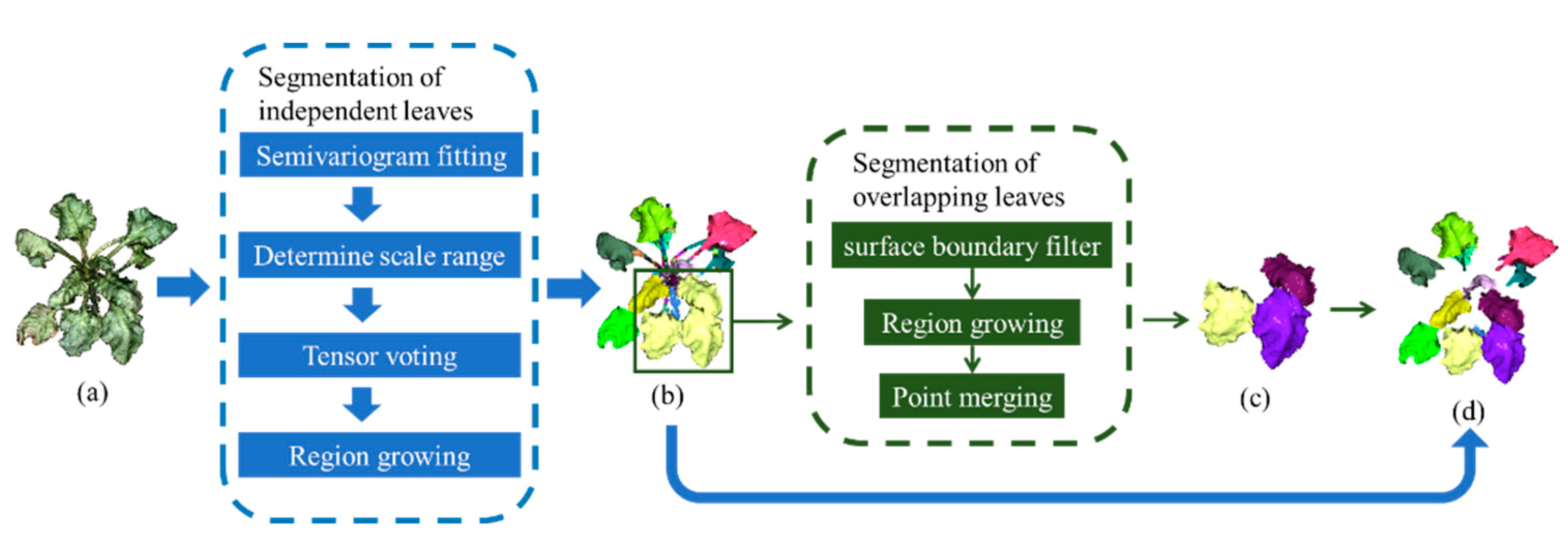
2.3. Point Cloud Segmentation of Individual Leaves

Individual leaves can be separated into two groups (Figure 2): independent leaves and overlapping leaves. Point cloud segmentation of individual leaves is implemented in Python 3.7 with sklearn [35] and open3d [36] libraries. The operating environment is Intel-10750 H CPU, 16 GB DRAM. The operating system is Windows 10.

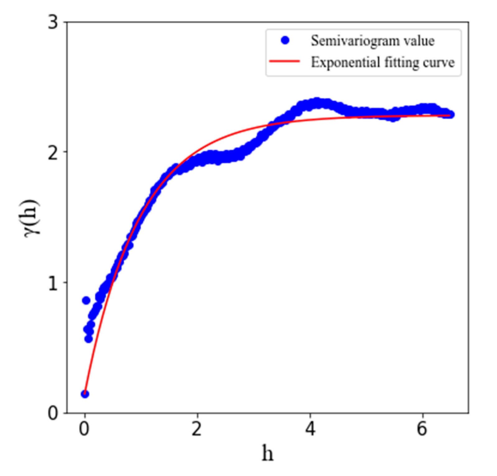
2.3.1. Point Cloud Segmentation of Independent Leaves

The region-growing algorithm [37] usually uses the point with the smallest curvature as the initial seed point [38]. Due to the influence of natural wrinkles and bending on the surface of sugar beet leaves for the calculation of curvature, it is necessary to adopt a criterion that can reflect the ‘smoothness’ of sugar beet leaves for the selection of initial seed points. This criterion should tolerate uneven folds on ‘smooth’ leaves and effectively distinguish plant leaves with stems. In this paper, the multiscale tensor voting method (MSTVM)-based region-growing algorithm is used to segment the point cloud of sugar beet leaves [39].

The calculated strength of the comprehensive plane feature is used as the initial seed point selection criterion. In MSTVM, multiscale means that the range of tensor voting is not unique. The voting size ${\mu }_i$ of the point $P_i$ in the 3D point cloud is attenuated by the Gaussian function:

$${\mu }_i=e^{\left(-\frac{s_j^2}{{\sigma }^2}\right)}$$

(1)

where $s_j$ is the distance of the voter to the receiver. The scale parameter $\sigma$ influences the voting range and the number of adjacent points and is very important for the correct acquisition of the 3D structural features of point position $P_i$ [40]. In this research, scale parameter $\sigma$ is determined by the semivariogram. To calculate the semivariogram value $\gamma \left(h\right)$ of the given point cloud and fit the exponential model Formula (2), methods used by Wu et al. [39] were adopted.

$$\gamma \left(h\right)=C_0+C\left(1-e^{-\frac{h}{b}}\right)$$

(2)

where $b$ is a constant value associated with range, range is the lag distance where the model first flattens out. Nugget $C_0$ is the intercept of the semivariogram model on the y axis. The value that the semivariogram model attains at the range is called the sill, represented by $C_0+C$. When $h$ approaches 0, $\gamma \left(h\right)$ reaches nugget $C_0$; when $h$ approaches $3b$, $\gamma \left(h\right)$ reaches 95% of sill $C_0+C$ [41]; when $h$ approaches maximum, $\gamma \left(h\right)$ reaches sill $C_0+C$. For Formula (2), it was shown that “when $h$ increases to $3b$, the plane feature strength can be more accurately calculated since the search region and the detection plane are essentially the same size” [39]. In this paper, the range of the scale parameter $\sigma$ was selected as $\left(0, 3b\right]$. When $\sigma$ is determined, the voting size ${\mu }_i$ of the point $P_i$ is then calculated.

Then, tensor voting is performed within the voting size ${\mu }_i$ of point $P_i$. Tensor voting has some certain resistance to noise [42]. The algorithm first encodes the points, and then infers the 3D geometric structure of the points based on the results of the information propagation between the points and the surrounding points. In tensor voting, the tensor (voter) corresponding to each point $P_i$ spreads its information to the tensor (receiver) corresponding to other points within the voting size of ${\mu }_i$ in the form of ball voting. The voting tensor $T_i$ of point $P_i$ can be calculated by Equation (3) [43]:

$$T_i={\displaystyle \sum }_{j\in N\left(i\right)}{\mu }_j\left(I_3-\frac{{\mathit{v}}_{\mathit{j}}{\mathit{v}}_{\mathit{j}}^{\mathit{T}}}{\Vert {\mathit{v}}_{\mathit{j}}{\mathit{v}}_{\mathit{j}}^{\mathit{T}}\Vert }\right)$$

(3)

where $I_3$ is an identity matrix, ${\mathit{v}}_{\mathit{j}}$ is the vector which connects to the receiver. After the information propagation at voting size ${\mu }_i$ is over, the symmetric and positive semi-definite 3 × 3 matrix $T$ can be decomposed according to Formula (4) and the 3D structure around the point can be inferred.

$$T=\left({\lambda }_1-{\lambda }_2\right){\mathit{e}}_{\mathbf{1}}{\mathit{e}}_{\mathbf{1}}^{\mathit{T}}+\left({\lambda }_2-{\lambda }_3\right)\left({\mathit{e}}_{\mathbf{1}}{\mathit{e}}_{\mathbf{1}}^{\mathit{T}}+{\mathit{e}}_{\mathbf{2}}{\mathit{e}}_{\mathbf{2}}^{\mathit{T}}\right)+{\lambda }_3\left({\mathit{e}}_{\mathbf{1}}{\mathit{e}}_{\mathbf{1}}^{\mathit{T}}+{\mathit{e}}_{\mathbf{2}}{\mathit{e}}_{\mathbf{2}}^{\mathit{T}}+{\mathit{e}}_{\mathbf{3}}{\mathit{e}}_{\mathbf{3}}^{\mathit{T}}\right)$$

(4)

where ${\lambda }_{\mathrm{i}}$ is the eigenvalue corresponding to the eigenvector ${\mathit{e}}_{\mathit{i}}$ (i = 1, 2, 3).

According to the spectrum theorem [44], combinations of different eigenvalues can represent various local structure features. In the segmentation of the point cloud of sugar beet plants, the plane features are the most concerned. The plane feature strength $\phi$ [45] used in this paper is defined as:

$$\phi =\frac{\left({\lambda }_1-{\lambda }_2\right)}{{\lambda }_1}$$

(5)

In order to calculate the comprehensive plane feature corresponding to the point $P_i$, the plane feature strength ${\phi }_i=\left({\phi }_{i1},{\phi }_{i2},\dots ,{\phi }_{im}\right)$ of the point $P_i$ in scales of $\sigma$ is calculated. There are $\mathrm{m}$ different scales within $\left(0, 3b\right]$ which is the range of the scale parameter $\sigma$. The comprehensive plane feature strength ${\phi }_i^{\prime }$ of point $p_i$ can be calculated according to Formula (6):

$${\phi }_i^{\prime }=\frac{\left({{\displaystyle \sum }}_{j=1}^m{\phi }_{ij}\right)}{m}$$

(6)

where ${\phi }_i^{\prime }$ is the comprehensive plane feature strength of $P_i$. When it is greater than the set threshold, this point can be judged as the initial seed point and be used in the region-growing algorithm.

Taking the sugar beet plant shown in (Figure 1a) as an example, the calculation result of the semivariogram value was shown by the blue dots in (Figure 3), and the fitting curve was shown by the red line, which gave $\gamma \left(h\right)=0.14+1.99\left(1-e^{-\frac{h}{0.91}}\right)$. Therefore, the range of the scale parameter $\phi$ was $\left(0, 2.73\right]$. When the MSTVM was executed, the number of different scales m was set to 5, $\sigma =\left(0.5, 1.0, 1.5, 2.0, 2.5\right)$.

After the initial seed points are determined, the region growing process from the seed point with the largest comprehensive plane feature strength is used to determine the segmentation area where this seed point is located. If the angle between the normal vector of the neighboring point and the seed point is less than the threshold ${\theta }_{th}$, the neighboring point will be merged into the segmentation area. At the same time, the curvature of the neighboring point is calculated. If the curvature is less than the curvature threshold $c_{th}$, the neighboring point is used as the next seed point of the segmented region to continue the region growing process, otherwise the point is ignored. The above process will be repeated until the area reaches the maximum value. Once this segmented area is determined, the region growing process is proceeded from the next initial seed point to repeat the above process until all initial seed points are processed. The angle threshold ${\theta }_{th}$ of normal vector is an empirical value selected based on the calculation results, and the curvature threshold $c_{th}$ is 95% of the curvature value of each point in the point cloud after sorting in ascending order [46]. The purpose of using threshold in this paper is to keep a balance between over-segmentation and under-segmentation. Finally, all the leaf areas are saved, including the individual leaf point clouds that has been segmented and the overlapping leaf point clouds that need further segmentation.

2.3.2. Point Cloud Segmentation of Overlapping Leaves

In this study, we use the SBF method to segment overlapping leaves. The SBF uses the principal component analysis (PCA) to extract edge points of the curved surface and performs well when applied to plant leaves [47].

In one filter process, SBF searches the edge points of overlapping leaves. Specifically, for the point $P_i$ to be processed in the point cloud, $P_i$ and its k-nearest neighbors $P_j\left(j=1,2,3\dots k\right)$ are projected to the principal plane obtained by PCA. Then, projected point $X_i$ and projected k-nearest neighbors $X_j\left(j=1,2,3\dots k\right)$ are calculated and all the angles between any two adjacent vectors $X_j-X_i$ are saved. If the maximum adjacent angle difference is greater than the set threshold, the point $P_i$ will be judged as an edge point. The above process is then repeated for the unprocessed points. Finally, all the edge points are temporarily removed.

After multiple filtering, enough points of the leaf overlap boundary are removed by the SBF, and the remaining part of each leaf are completely separated from each other. Then, the region-growing algorithm is applied to the remaining part to distinguish each leaf region. Finally, temporarily removed points are merged into different leaf regions with the criterion that whether more than 50% of the points in the neighborhood belong to one of the leaf regions.

2.4. Performance Evaluation of Phenotypic Data Extraction

The specific calculation methods for leaf length and leaf area are as follows:

The leaf length is calculated according to Xiao et al. [6]. The approximate shortest curve between the tip point and the base point of the leaf point cloud is searched. The curve is then projected and fitted, and the length of the calculated curve is the leaf length.

The Helen formula (Equation (7)) [48] is used to calculate the area of a single triangle.

$$S=\sqrt{p\ast \left(p-a\right)\ast \left(p-b\right)\ast \left(p-c\right)}$$

(7)

where S is the area of a triangle, p is the half of perimeter of this triangle and a, b, and c are the lengths of the three sides of this triangle. The estimated area of individual leaf was calculated by adding all the triangles belong to this leaf.

Manually segmented leaf point clouds were used as a reference to calculate the accuracy, recall, and F1-Score in order to evaluate the model performance. These performance metrics evaluated based on leaf-to-leaf comparison.

$$\mathrm{Accuracy}:p=\frac{TP}{\left(TP+FP\right)}$$

(8)

$$\mathrm{Recall}:r=\frac{TP}{\left(TP+FN\right)}$$

(9)

$$\mathrm{F}1-\mathrm{Score}:\mathit{F1}-\mathit{Score}=\frac{2\ast p\ast r}{p+r}$$

(10)

Correlation coefficient R², Mean Absolute Percentage Error (MAPE), and Root Mean Square Error (RMSE) were also calculated to evaluate the accuracy of extracted phenotypic data.

$$MAPE\left(X,h\right)=\frac{100\%}{n}{\displaystyle \sum }_{i=1}^n\frac{\left|h\left(x_i\right)-y_i\right|}{y_i}$$

(11)

$$RMSE\left(X,h\right)=\sqrt{\frac{1}{n}{\displaystyle \sum }_{i=1}^n{\left(h\left(x_i\right)-y_i\right)}^2}$$

(12)

where n is the number of samples; $h\left(x_i\right)$ and $y_i$ are the estimation value and manual measurement, respectively.

The measured leaf area of individual sugar beet was calculated with (Equation (13)) [49]:

Leaf area = L × W × k

(13)

where L is the measured leaf length, W is the measured maximum leaf width, and k is the Montgomery parameter with 0.802 here [50].

3. Results

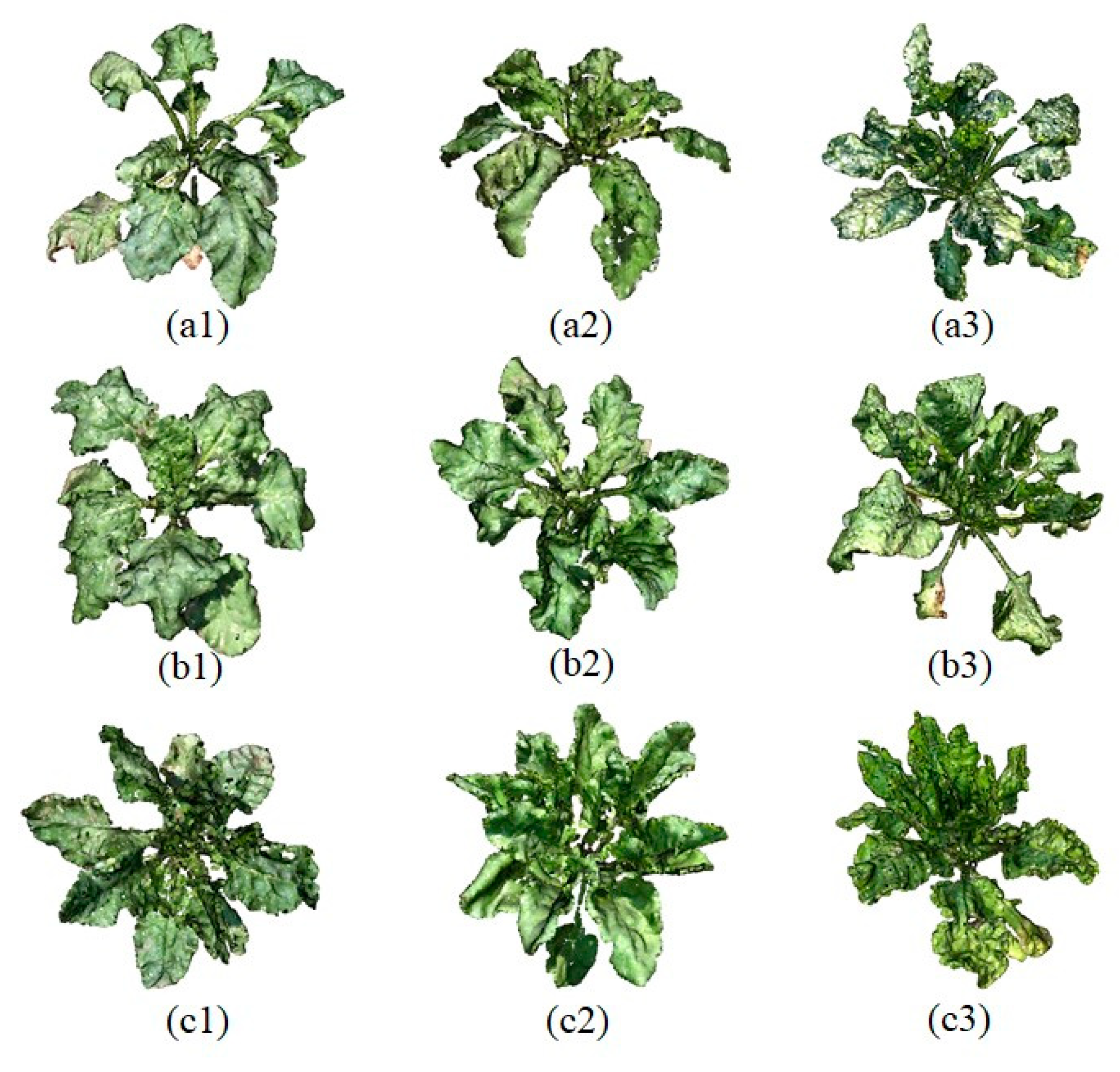
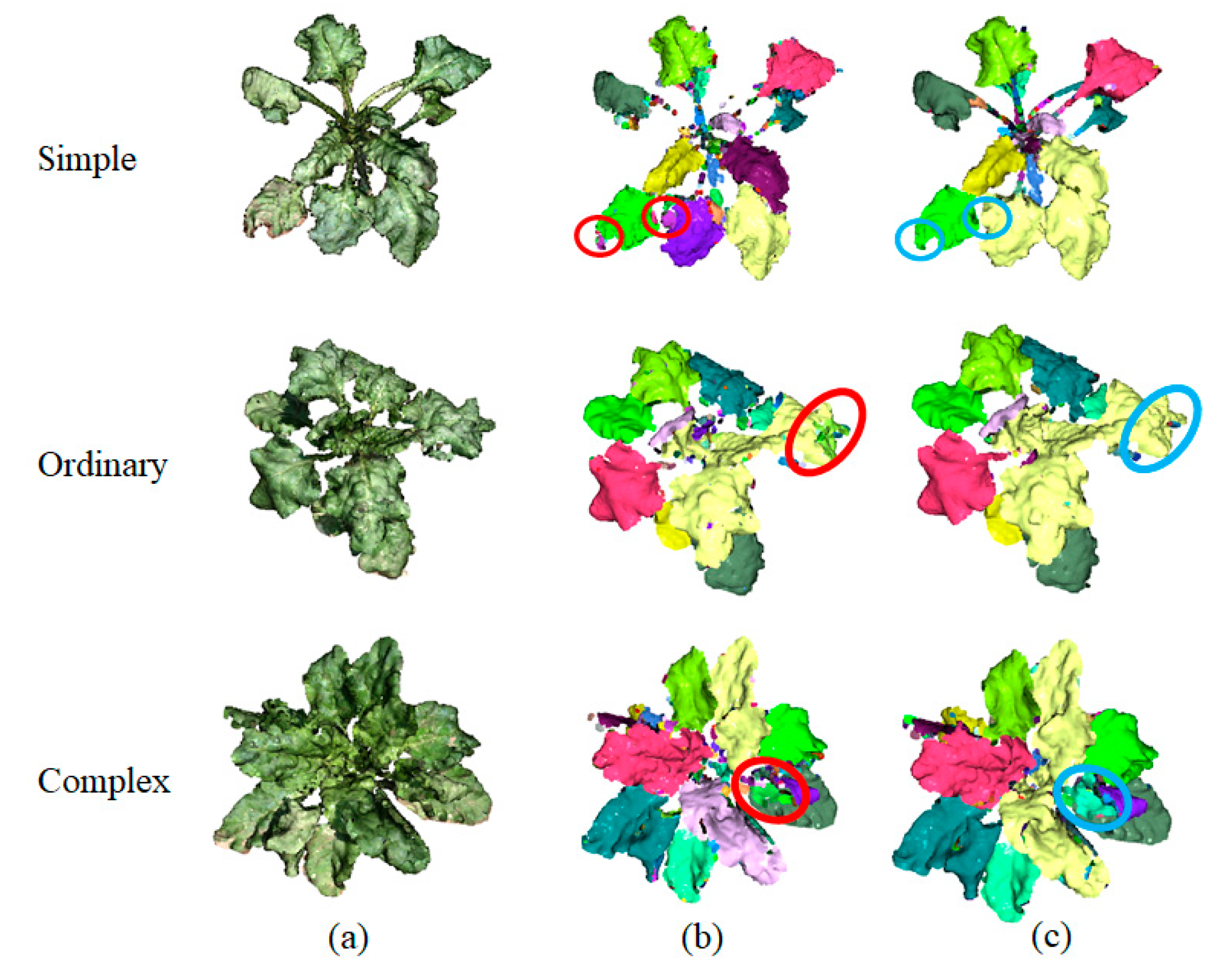
3.1. Segmentation of Individual Leaves with MSTVM-Based Region-Growing Algorithm

To verify the segmentation effect to sugar beet plants with different complexity of leaf layout, three categories were divided with the 3D point clouds based on the complexity of the leaf layout: simple structure with no more than three overlapping leaves in one overlapping area (hereafter referred to as simple), ordinary structure with 3~5 overlapping leaves in one overlapping area (hereafter referred to as ordinary), and complex structure with more than five overlapping leaves in one overlapping area overlapping of leaves (hereafter referred to as complex). The examples of the three plant types were shown in (Figure 4). The total numbers of simple, ordinary, and complex plant types evaluated were 9, 13, and 8, respectively.

Both the region-growing algorithm and the MSTVM-based region-growing algorithm were used to segment the point clouds of 30 sugar beets, as shown in Figure 5. The only difference between these two algorithms was the selection criteria of seed points. All other parameter values were the same. Based on visual checks, the MSTVM-based region-growing algorithm yielded more complete leaf point clouds as compared to the region-growing algorithm. (Figure 5a–c).

The manually segmented leaf point clouds were used to evaluate the performance of the two methods (

Table 1. The mean and standard deviation of precision, recall, and F1-Score values with region-growing algorithm and MSTVM-based region-growing algorithm.

Plant Categories	Simple			Ordinary			Complex
Accuracy Indicators	p	r	f1	p	r	f1	p	r	f1
Region-growing algorithm	0.97 ± 0.08	0.79 ± 0.17	0.86 ± 0.13	0.97 ± 0.05	0.78 ± 0.16	0.85 ± 0.11	0.96 ± 0.07	0.74 ± 0.18	0.82 ± 0.14
MSTVM-based region-growing algorithm	0.96 ± 0.08	0.85 ± 0.14	0.89 ± 0.11	0.96 ± 0.07	0.86 ± 0.12	0.90 ± 0.09	0.95 ± 0.09	0.85 ± 0.14	0.89 ± 0.10

Note: All results were calculated against manually segmented results. p: precision, r: recall, f1: F1-Score.

). The t-test was used to compare the average of precision, recall, and f1-score of these two methods (

Table 2. The t-test of precision, recall, and F1-Score values with region-growing algorithm and MSTVM-based region-growing algorithm.

Plant Categories	Simple			Ordinary			Complex
Accuracy Indicators	p	r	f1	p	r	f1	p	r	f1
T	−1.33	5.29	4.08	−2.91	8.48	6.12	−2.21	9.90	7.31
p	0.18	0.00 *	0.00 *	0.00 *	0.00 *	0.00 *	0.03 *	0.00 *	0.00 *

Note: * indicates a significance level of 0.05.

). In addition, the results of Table 1 were expressed in boxplots (Figure 6). It could be seen that the MSTVM-based region-growing algorithm has an average F1-Score between 0.89 and 0.90 for the three categories of sugar beet plants, an average precision between 0.95 and 0.96, and an average recall value between 0.85 and 0.86, respectively. Compared with the region-growing algorithm, the average recall value increased, and the standard deviation decreased slightly, suggesting that the MSTVM-based region-growing algorithm performed better in segmenting relatively simple and ordinary leaves.

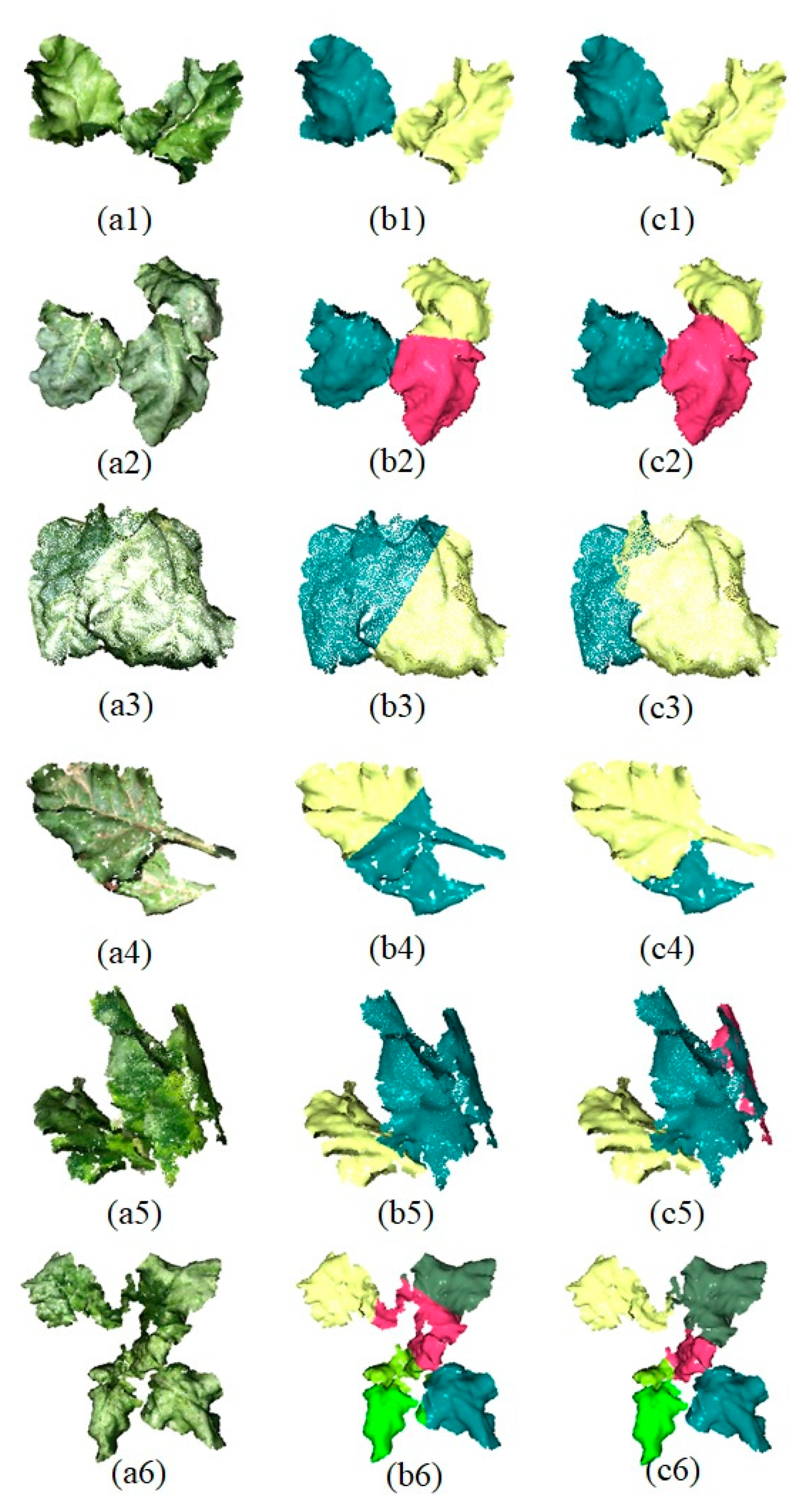
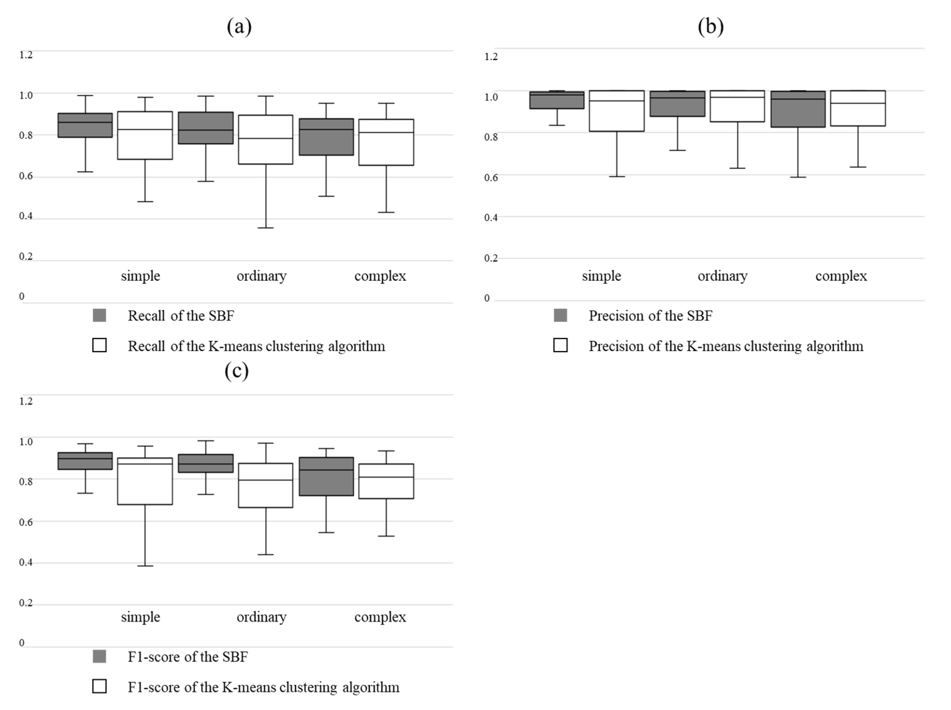
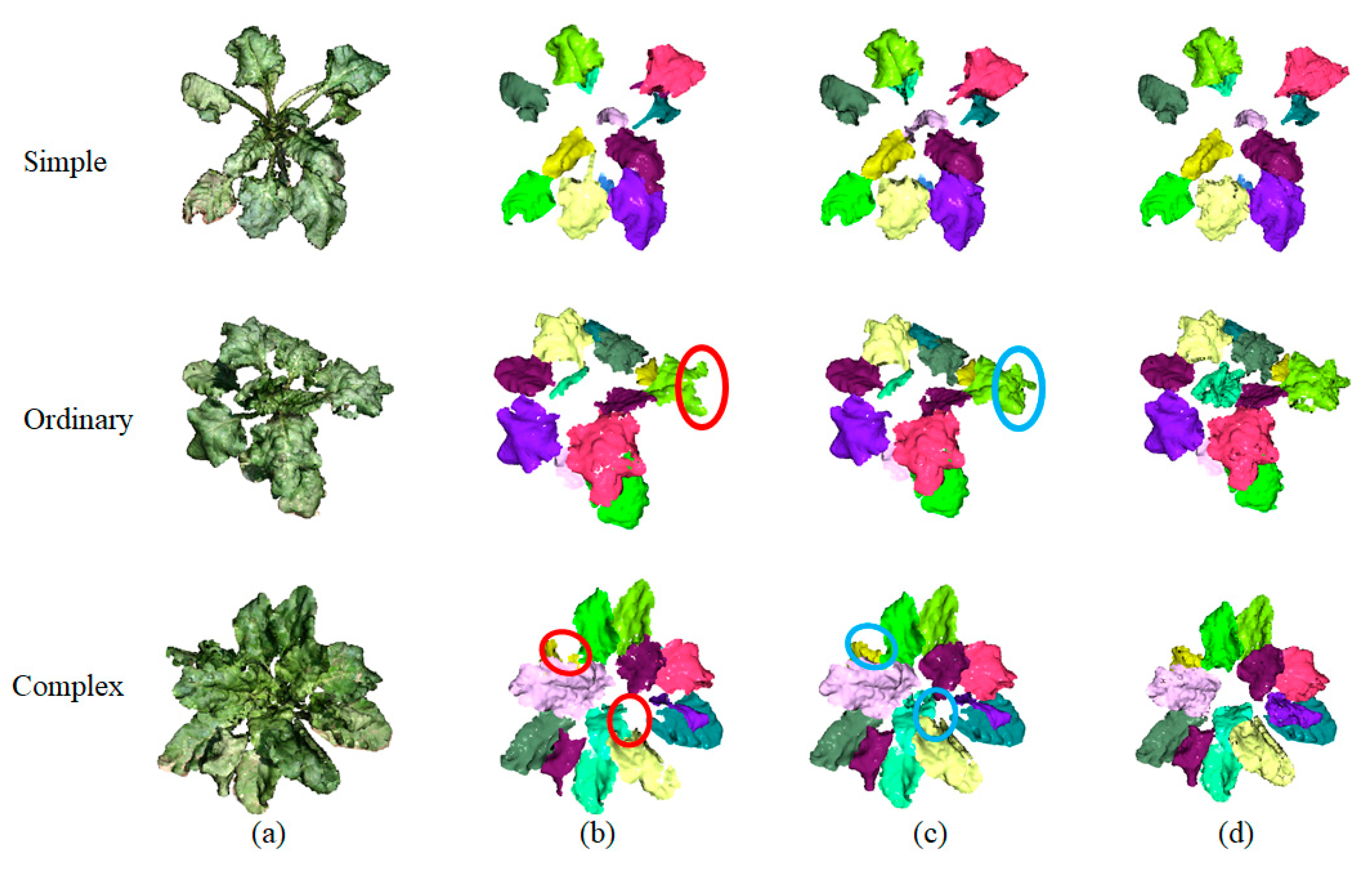
3.2. Further Segmentations for Overlapping Leaves

K-means clustering algorithm and SBF were further used to separate the overlapping leaves based on the results from the MSTVM-based region-growing algorithm (Figure 7). The purpose of using k-means clustering algorithm was to evaluate the performance of the SBF. The value of k in k-means algorithm was selected manually. K-means algorithm could obtain reasonable segmentation results when the overlapping leaves were similar in size and the overlaps between leaves were less (Figure 7(a2)). The performance of K-means algorithm was poor when the overlaps between leaves were large or the difference in leaf size was large (Figure 7(b2–b4)). Particularly, K-means algorithm could not accurately segment each leaf from multiple overlapped leaves (Figure 7(a5,a6)). SBF performed much better than K-means and six groups of data were shown in (Figure 7). Particularly, SBF could completely segment each complex overlapping leaf in (Figure 7(a6)). However, SBF is strongly influenced by the holes in the leaves, which the rightmost red leaf shown in (Figure 7(a5)) was separated into two leaves due to the large holes on that leaf.

Table 3. The Mean and standard deviation of segmented overlapping leaves by SBF and K-means clustering algorithm.

Plant Categories	Simple			Ordinary			Complex
Accuracy Indicators	p	r	f1	p	r	f1	p	r	f1
K-means	0.88 ± 0.15	0.79 ± 0.14	0.79 ± 0.16	0.88 ± 0.16	0.77 ± 0.15	0.76 ± 0.15	0.87 ± 0.16	0.76 ± 0.15	0.75 ± 0.15
SBF	0.93 ± 0.12	0.83 ± 0.12	0.87 ± 0.13	0.93 ± 0.11	0.81 ± 0.14	0.86 ± 0.11	0.91 ± 0.12	0.79 ± 0.14	0.83 ± 0.11

Note: All results were calculated against manually segmented results. p: precision, r: recall, f1: F1-Score.

evaluated the performance of SBF and K-means clustering algorithm in segmenting overlapping leaves. The t-test was used to compare the average of precision, recall, and f1-score of these two methods (

Table 4. The t-test of precision, recall, and F1-Score values of segmented overlapping leaves by SBF and K-means clustering algorithm.

Plant Categories	Simple			Ordinary			Complex
Accuracy Indicators	p	r	f1	p	r	f1	p	r	f1
T	2.30	1.15	3.08	1.98	2.54	5.29	−0.32	0.51	1.84
p	0.03 *	0.26	0.01 *	0.05 *	0.01 *	0.00 *	0.75	0.60	0.07

Note: * indicates a significance level of 0.05.

). In addition, the results of Table 3 were expressed in boxplots (Figure 8). The SBF method produced a higher F1-Score, ranging from 0.83 to 0.97, a precision value ranging from 0.91 to 0.93, and a recall value ranging from 0.79 to 0.83, respectively, as shown in Table 3. The corresponding indicators for K-means were 0.75~0.79 for F1-Score, 0.87~0.88 for precision, 0.76~0.79 for recall. Compared with the K-means clustering algorithm, SBF has higher mean values and lower standard deviations, and performs better in the segmentation of overlapping leaves. The advantage of low standard deviations could be clearly seen from Figure 8.

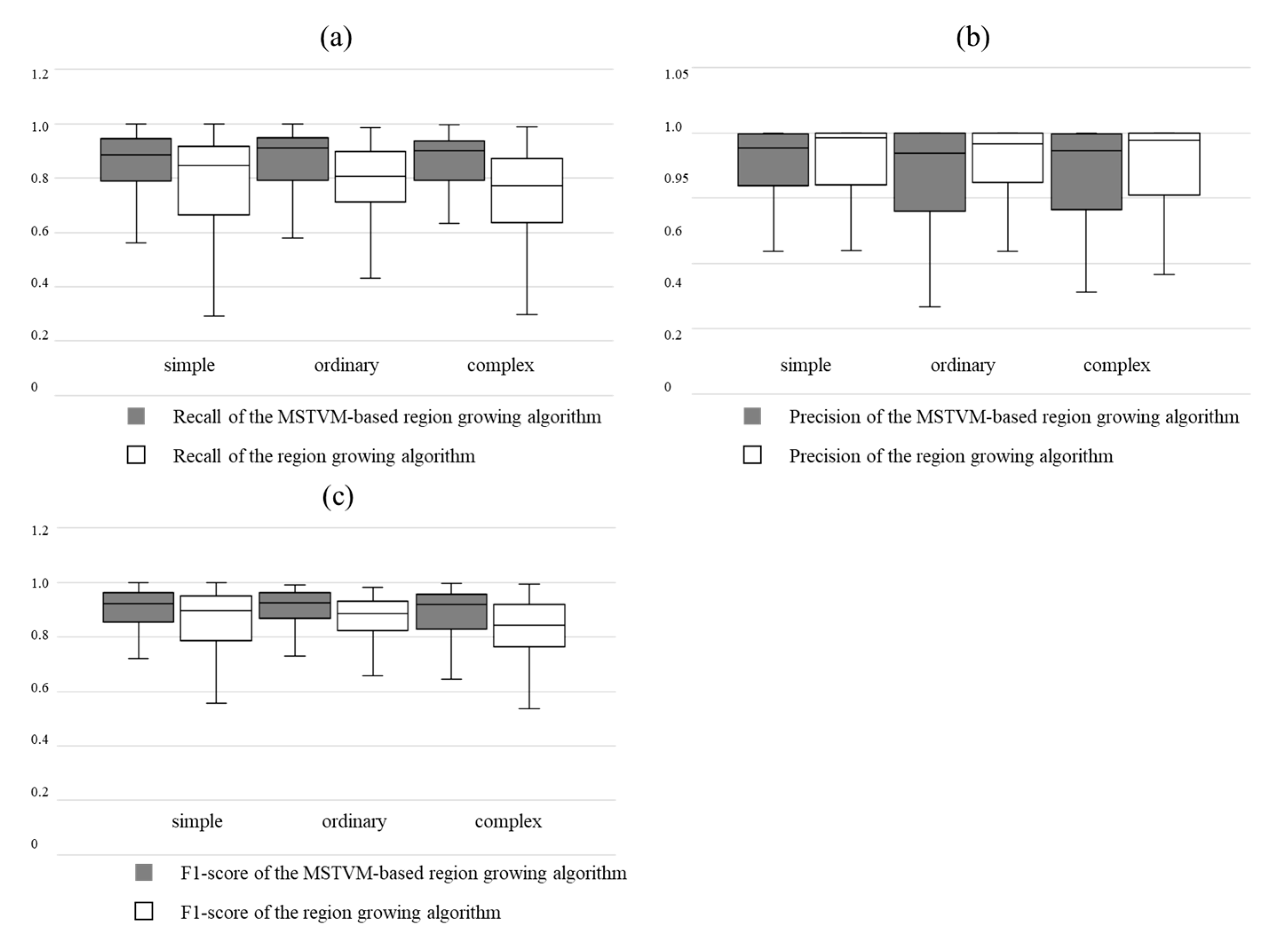
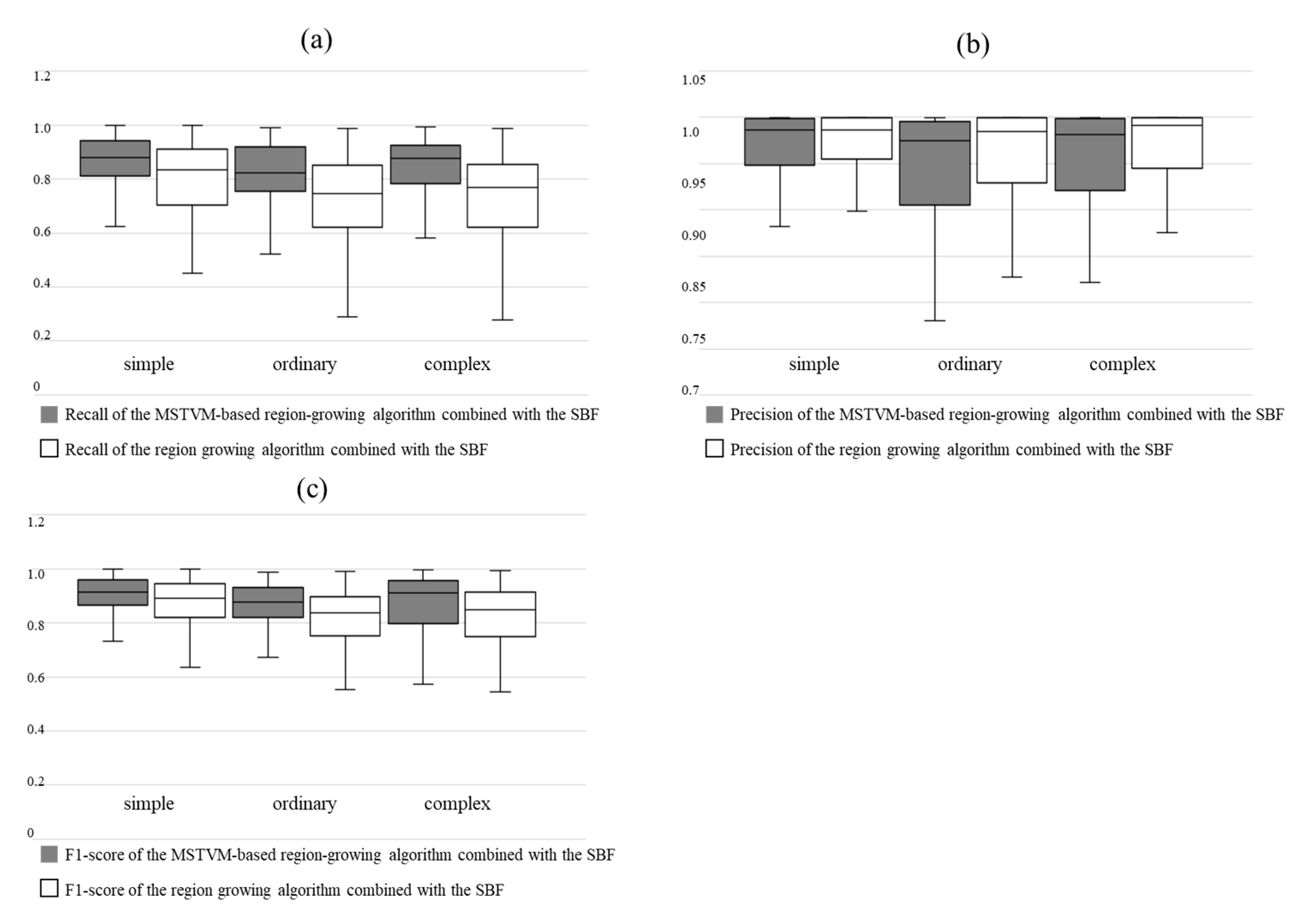
3.3. Evaluation of the Individual Leaf Segmentation for the Whole Plant

Figure 9 shows the results of simple, ordinary, and complex plant type structures created with a combination of different methods.

Table 5. The Mean and standard deviation of segmented leaves for the whole plant by the MSTVM-based region-growing algorithm combined with the SBF and by the region-growing algorithm combined with SBF.

Plant Categories	Simple			Ordinary			Complex
Accuracy Indicators	p	r	f1	p	r	f1	p	r	f1
Region-growing algorithm combined with SBF	0.96 ± 0.07	0.77 ± 0.17	0.84 ± 0.13	0.96 ± 0.05	0.75 ± 0.16	0.84 ± 0.11	0.95 ± 0.07	0.72 ± 0.17	0.81 ± 0.14
MSTVM-based region-growing algorithm combined with SBF	0.95 ± 0.09	0.84 ± 0.14	0.88 ± 0.11	0.95 ± 0.09	0.83 ± 0.13	0.89 ± 0.10	0.93 ± 0.10	0.83 ± 0.14	0.87 ± 0.10

Note: All results were calculated against manually segmented results. p: precision, r: recall, f1: F1-Score.

evaluated the performance of the region-growing algorithm combined with SBF and the MSTVM-based region-growing algorithm combined with SBF in segmenting the individual leaf of the whole plant. The t-test was used to compare the average of precision, recall, and f1-score of these two methods (

Table 6. The t-test of precision, recall, and F1-Score values of segmented leaves for the whole plant by the MSTVM-based region-growing algorithm combined with SBF and by the region-growing algorithm combined with SBF.

Plant Categories	Simple			Ordinary			Complex
Accuracy Indicators	p	r	f1	p	r	f1	p	r	f1
T	−1.99	6.51	4.44	−2.71	9.88	7.22	−3.04	11.04	7.51
p	0.05 *	0.00 *	0.00 *	0.01 *	0.00 *	0.00 *	0.03 *	0.00 *	0.00 *

Note: * indicates a significance level of 0.05.

). The results of Table 5 were expressed in boxplots (Figure 10). Compared with the region-growing algorithm combined with SBF in (Figure 9b,c), leaf segmentation with the MSTVM-based region-growing algorithm combined with SBF was more accurate, as shown in blue circles in (Figure 9c) with a higher F1-Score (0.87~0.89), precision (0.93~0.95), and recall values (0.83~084), and a lower standard deviation. The corresponding evaluation indicators for the region-growing algorithm combined with SBF were 0.81~0.84, 0.95~0.96, and 0.72~0.77, respectively. From Figure 10, it can be clearly seen that the effect of the MSTVM-based region-growing algorithm combined with SBF was better.

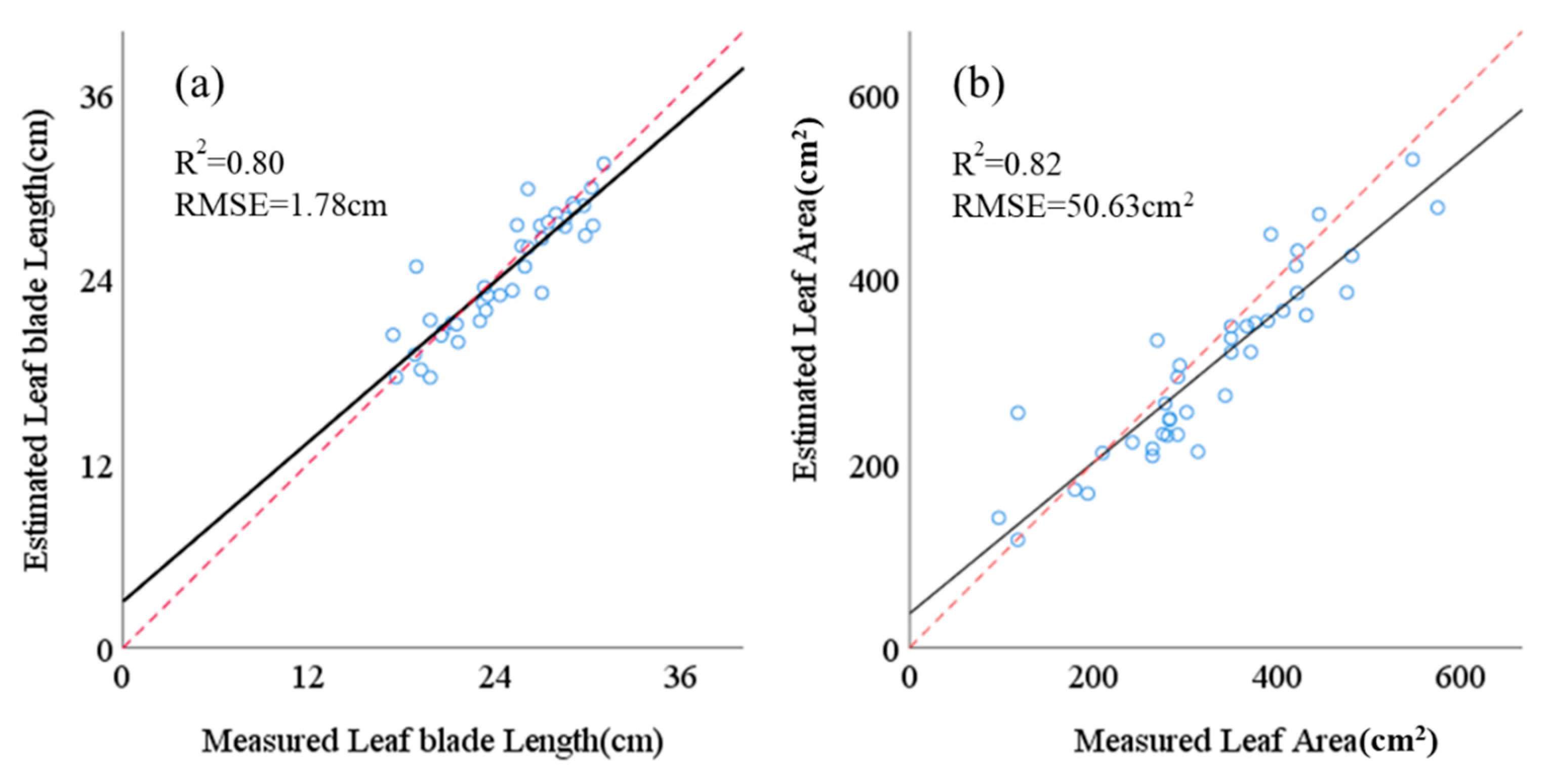
3.4. Evaluation of Extracted Phenotypic Data

The leaf blade length and leaf area of an individual leaf were calculated based on the best method identified above by the MSTVM-based region-growing algorithm combined with SBF and compared with the measured leaf length and leaf area (Figure 11). The linear fitting equation between the calculated and the measured leaf length is y = 0.92x + 2.04 with a correlation coefficient R² of 0.80, RMSE of 1.78 cm, and MAPE of 5.27%, respectively. The linear fitting equation between calculated and measured leaf area is y = 0.82x + 36.86. The corresponding R² is 0.82, RMSE is 50.63 cm², and MAPE is 14.61%.

4. Discussion

The reason why this paper uses the SFM algorithm to generate point clouds is that it has the advantages of a low cost, simple use, and robustness [20]. Before point cloud segmentation, background points such as soil and shadows should be removed, to obtain clean plants and to avoid the interference to the proposed method. Xiao et al. [7] used color filter to remove soil and shadows points. However, this method cannot remove all the background points, and instead removes some of the plant points. Therefore, we removed the background points from the sugar beet plant group manually. The region-growing algorithm has been applied to the segmentation of 3D point cloud of plants with smooth leaf surfaces such as eggplant [51] and maize [52]. However, the region-growing algorithm is unable to acquire accurate segmentation for field grown sugar beet leaves due to the existence of leaf curvatures and serious overlapping within individual plant. Xiao et al. [7] used a clustering algorithm to cluster the discarded points into different leaf regions after segmentation of region-growing algorithm, but the effect of clustering was not evaluated, and the segmentation of overlapping leaves was not considered.

In order to resolve the incomplete segmentation of leaf point cloud caused by folds on the surface of sugar beet leaves, this paper used the MSTVM, a multi-scale processing method, to calculate the comprehensive plane feature strength of each point in the input point cloud as the seed point selection criterion for the region-growing algorithm. Due to the fact that the calculation of the comprehensive plane feature strength was carried out at multiple scales, the selected seed points produced a smoother leaf surface. The results showed that selection methods of seed points improved the performance of the region-growing algorithm. The F1-Score increased from 0.82~0.86 to 0.89~0.90, and the standard deviation was reduced (Table 1).

The MSTVM-based region-growing algorithm performed poorly in the segmentation of overlapping leaves. Most of overlapping leaves in the reconstructed 3D point cloud of sugar beet plants were horizontal overlapped, which was favorable for PCA projection and the accurate operation of SBF. Therefore, we used the SBF to segment the overlapping leaves and compared its performance with the K-means clustering algorithm. Compared with other machine learning methods such as SVM [53] and boosting [54], the K-means clustering algorithm is superior in processing efficiency and segmentation accuracy in the segmentation of overlapping leaves [55].

Due to the mutual occlusion between sugar beet leaves, there are holes in SFM reconstructed leaf point clouds. This situation will cause the SBF method to mistake the points of the hole edge as the ones of leaf edge, then remove them mistakenly. In order to reduce the impact of these holes in the overlapping leaf point cloud during the filter operation, a fixed radius is used when searching for the neighboring points of the point $P_i$ in the overlapping leaf point cloud [47]. Compared with the K-means, the SBF increased the f1-score by 0.08, 0.10, and 0.08 on simple, ordinary and complex plant categories, respectively (Table 3). In this paper, the SBF was used to segment overlapping leaf point clouds obtained by the MSTVM-based region-growing algorithm. However, improvement in the performance of the severe occlusion between leaves is still needed as shown in (Figure 7(a5,a6)). The 3D space information of the leaf edge will be further combined to deal with the severe occlusion. The leaf length and leaf area extracted based on individual leaves after segmentation agree well with the measurements with high accuracy. Elnashef et al. [23] had used the automatic segmentation on crops that were characterized by narrow leaves and tillers, and conducted experiments on cotton, maize and wheat seedlings. It could potentially be used in high-throughput phenotypic data acquisition. In the existing research [19,20,25,27,56], the point cloud data of the early-growth plant was used to divide the leaves with simple plant structures. This study directly segmented the sugar beet plants with different complexities of the plant leaf layout at different growth stages in the field with obvious leaf overlapping. The segmentation results showed the robustness of MSTVM-based region-growing algorithm combined with SBF in leaf segmentation.

In field experiment, the process of SFM method for image collection is laborious. The SFM method uses multi-view images to reconstruct point clouds, which requires adjacent images with a certain degree of overlap. The camera carrier must move around the plant while capturing the image at a constant speed. To save labor costs, we will consider using drones to collect imagery in the future. One of the limitations about the experiment is the small amount of genotypes evaluated (only 20). Another is that the experiment does not have enough repetition and randomization. In the future, we will use more genotypes and repeat these genotypes in several plots in the same experimental area to verify the effectiveness of the method. Furthermore, we will improve the automation of the entire process and increase the processing speed, meanwhile ensuring the accuracy of calculation so as to provide high-throughput analysis methods for the phenotypic data acquisition of more complex plants in the field.

5. Conclusions

In this study, the 3D point clouds were divided into three categories based on the complexity of the plant leaf layout. The combination of the MSTVM-based region-growing algorithm with SBF was used to achieve the point cloud segmentation of an individual leaf of a field sugar beet plant. The MSTVM was used to calculate the comprehensive plane feature. The SBF method was used to process the overlapping leaf point cloud. For the point clouds of 30 field grown sugar beet plants, this method achieved a F1-score of 0.87~0.89, recall of 0.83~0.84, and precision of 0.93~0.95. Based on the individual leaf obtained by the method, the calculated leaf length and leaf were correlated well with the measurement (R² = 0.80~0.82). This method could be used as an efficient leaf segmentation method which is a basic step for the phenotypic analysis of plants with complex leaf layouts and would be particularly useful for sugar beet breeding.

References

1. Brar, N.; Dhillon, B.; Saini, K.S.; Sharma, P. Agronomy of sugarbeet cultivation—A review. Agric. Rev. 2015, 36, 184–197. [Google Scholar] [CrossRef]
2. Zhang, Y.; Nan, J.; Yu, B. OMICS technologies and applications in sugar beet. Front. Plant Sci. 2016, 7, 900. [Google Scholar] [CrossRef] [PubMed] [Green Version]
3. Furbank, R.T.; Tester, M. Phenomics–technologies to relieve the phenotyping bottleneck. Trends Plant Sci. 2011, 16, 635–644. [Google Scholar] [CrossRef]
4. Phillips, R.L. Mobilizing science to break yield barriers. Crop Sci. 2010, 50, 99–108. [Google Scholar] [CrossRef] [Green Version]
5. Dohm, J.C.; Minoche, A.E.; Holtgräwe, D.; Capella-Gutiérrez, S.; Zakrzewski, F.; Tafer, H.; Rupp, O.; Sörensen, T.R.; Stracke, R.; Reinhardt, R.; et al. The genome of the recently domesticated crop plant sugar beet (Beta vulgaris). Nature 2014, 505, 546–549. [Google Scholar] [CrossRef] [PubMed] [Green Version]
6. White, J.W.; Andrade-Sanchez, P.; Gore, M.A.; Bronson, K.F.; Coffelt, T.A.; Conley, M.M.; Feldmann, K.A.; French, A.N.; Heun, J.T.; Hunsaker, D.J.; et al. Field-based phenomics for plant genetics research. Field Crop. Res. 2012, 133, 101–112. [Google Scholar] [CrossRef]
7. Xiao, S.; Chai, H.; Shao, K.; Shen, M.; Wang, Q.; Wang, R.; Sui, Y.; Ma, Y. Image-based dynamic quantification of aboveground structure of sugar beet in field. Remote Sens. 2020, 12, 269. [Google Scholar] [CrossRef] [Green Version]
8. Wang, N.; Wu, X.; Ku, L.; Chen, Y.; Wang, W. Evaluation of Three protein-extraction methods for proteome analysis of maize leaf midrib, a compound tissue rich in sclerenchyma cells. Front. Plant Sci. 2016, 7, 856. [Google Scholar] [CrossRef] [PubMed] [Green Version]
9. Weight, C.; Parnham, D.; Waites, R. TECHNICAL ADVANCE: LeafAnalyser: A computational method for rapid and large-scale analyses of leaf shape variation. Plant J. 2008, 53, 578–586. [Google Scholar] [CrossRef]
10. Granier, C.; Aguirrezabal, L.; Chenu, K.; Cookson, S.J.; Dauzat, M.; Hamard, P.; Thioux, J.; Rolland, G.; Bouchier-Combaud, S.; Lebaudy, A.; et al. PHENOPSIS, an automated platform for reproducible phenotyping of plant responses to soil water deficit in Arabidopsis thaliana permitted the identification of an accession with low sensitivity to soil water deficit. New Phytol. 2006, 169, 623–635. [Google Scholar] [CrossRef]
11. Gibbs, J.A.; Pound, M.; French, A.P.; Wells, D.M.; Murchie, E.; Pridmore, T. Plant phenotyping: An active vision cell for three-dimensional plant shoot reconstruction. Plant Physiol. 2018, 178, 524–534. [Google Scholar] [CrossRef] [PubMed] [Green Version]
12. Li, H.; Qian, Y.; Cao, P.; Yin, W.; Dai, F.; Hu, F.; Yan, Z. Calculation method of surface shape feature of rice seed based on point cloud. Comput. Electron. Agric. 2017, 142, 416–423. [Google Scholar] [CrossRef]
13. Wu, G.; Li, B.; Zhu, Q.; Huang, M.; Guo, Y. Using color and 3D geometry features to segment fruit point cloud and improve fruit recognition accuracy. Comput. Electron. Agric. 2020, 174, 105475. [Google Scholar] [CrossRef]
14. Paulus, S. Measuring crops in 3D: Using geometry for plant phenotyping. Plant Methods 2019, 15, 103. [Google Scholar] [CrossRef] [PubMed]
15. Jin, S.; Su, Y.; Gao, S.; Wu, F.; Ma, Q.; Xu, K.; Hu, T.; Liu, J.; Pang, S.; Guan, H.; et al. Separating the structural components of maize for field phenotyping using terrestrial lidar data and deep convolutional neural networks. IEEE Trans. Geosci. Remote Sens. 2020, 58, 2644–2658. [Google Scholar] [CrossRef]
16. Bao, Y.; Tang, L.; Srinivasan, S.; Schnable, P.S. Field-based architectural traits characterisation of maize plant using time-of-flight 3D imaging. Biosyst. Eng. 2019, 178, 86–101. [Google Scholar] [CrossRef]
17. Jin, S.; Su, Y.; Wu, F.; Pang, S.; Gao, S.; Hu, T.; Liu, J.; Guo, Q. Stem-leaf segmentation and phenotypic trait extraction of individual maize using terrestrial LiDAR data. IEEE Trans. Geosci. Remote Sens. 2019, 57, 1336–1346. [Google Scholar] [CrossRef]
18. Xiang, L.; Bao, Y.; Tang, L.; Ortiz, D.; Salas-Fernandez, M.G. Automated morphological traits extraction for sorghum plants via 3D point cloud data analysis. Comput. Electron. Agric. 2019, 162, 951–961. [Google Scholar] [CrossRef]
19. Harmening, C.; Paffenholz, J. A Fully automated three-stage procedure for spatio-temporal leaf segmentation with regard to the B-spline-based phenotyping of cucumber plants. Remote Sens. 2021, 13, 74. [Google Scholar] [CrossRef]
20. Yang, Z.; Han, Y. A low-cost 3D phenotype measurement method of leafy vegetables using video recordings from smartphones. Sensors 2020, 20, 6068. [Google Scholar] [CrossRef]
21. Zhu, B.; Liu, F.; Xie, Z.; Guo, Y.; Li, B.; Ma, Y. Quantification of light interception within image-based 3-D reconstruction of sole and intercropped canopies over the entire growth season. Ann. Bot. 2020, 126, 701–712. [Google Scholar] [CrossRef] [Green Version]
22. Ghahremani, M.; Williams, K.; Corke, F.; Tiddeman, B.; Liu, Y.; Wang, X.; Doonan, J.H. Direct and accurate feature extraction from 3D point clouds of plants using RANSAC. Comput. Electron. Agric. 2021, 187, 106240. [Google Scholar] [CrossRef]
23. Elnashef, B.; Filin, S.; Lati, R.N. Tensor-based classification and segmentation of three-dimensional point clouds for organ-level plant phenotyping and growth analysis. Comput. Electron. Agric. 2019, 156, 51–61. [Google Scholar] [CrossRef]
24. Miao, T.; Zhu, C.; Xu, T.; Yang, T.; Li, N.; Zhou, Y.; Deng, H. Automatic stem-leaf segmentation of maize shoots using three-dimensional point cloud. Comput. Electron. Agric. 2021, 187, 106310. [Google Scholar] [CrossRef]
25. Liu, Z.; Zhang, Q.; Wang, P.; Li, Z.; Wang, H. Automated classification of stems and leaves of potted plants based on point cloud data. Biosyst. Eng. 2020, 200, 215–230. [Google Scholar] [CrossRef]
26. Gélard, W.; Herbulot, A.; Devy, M.; Debaeke, P.; McCormick, R.F.; Truong, S.K.; Mullet, J. Leaves Segmentation in 3D Point Cloud. In Proceedings of the International Conference on Advanced Concepts for Intelligent Vision Systems, Antwerp, Belgium, 8–21 September 2017; Springer: Cham, Switzerland, 2017. [Google Scholar]
27. Shi, W.; van de Zedde, R.; Jiang, H.; Kootstra, G. Plant-part segmentation using deep learning and multi-view vision. Biosyst. Eng. 2019, 187, 81–95. [Google Scholar] [CrossRef]
28. Liu, J.; Liu, Y.; Doonan, J. Point Cloud Based Iterative Segmentation Technique for 3D Plant Phenotyping. In Proceedings of the 2018 IEEE International Conference on Information and Automation, Wuyishan, China, 11–13 August 2018. [Google Scholar]
29. Dandrifosse, S.; Bouvry, A.; Leemans, V.; Dumont, B.; Mercatoris, B. Imaging wheat canopy through stereo vision: Over-coming the challenges of the laboratory to field transition for morphological features extraction. Front. Plant Sci. 2020, 11, 96. [Google Scholar] [CrossRef] [PubMed] [Green Version]
30. Müller-Linow, M.; Pinto-Espinosa, F.; Scharr, H.; Rascher, U. The leaf angle distribution of natural plant populations: Assessing the canopy with a novel software tool. Plant Methods 2015, 11, 11. [Google Scholar] [CrossRef] [PubMed] [Green Version]
31. Pinto, F.; Müller-Linow, M.; Schickling, A.; Cendrero-Mateo, M.P.; Ballvora, A.; Rascher, U. Multiangular observation of canopy sun-induced chlorophyll fluorescence by combining imaging spectroscopy and stereoscopy. Remote Sens. 2017, 9, 415. [Google Scholar] [CrossRef] [Green Version]
32. Scholz, O.; Uhrmann, F.; Wolff, A.; Pieger, K.; Penk, D. Determination of Detailed Morphological Features for Phenotyping of Sugar Beet Plants Using 3d-Stereoscopic Data. In Proceedings of the ISPRS Annals of Photogrammetry, Remote Sensing and Spatial Information Sciences 2019, Munich, Germany, 18–20 September 2019. [Google Scholar]
33. Lowe, D.G. Object recognition from scale-invariant keypoints. In Proceedings of the IEEE International Conference on Computer Vision 1999, Kerkyra, Corfu, Greece, 20–25 September 1999. [Google Scholar]
34. Fischler, M.A.; Bolles, R.C. Random sample consensus: A paradigm for model fitting with applications to image analysis and automated cartography. Commun. ACM 1981, 24, 381–395. [Google Scholar] [CrossRef]
35. Pedregosa, F.; Varoquaux, G.; Gramfort, A.; Michel, V.; Thirion, B.; Grisel, O.; Blondel, M.; Prettenhofer, P.; Weiss, R.; Dubourg, V.; et al. Scikit-learn: Machine learning in python. J. Mach. Learn. Res. 2011, 12, 2825–2830. [Google Scholar]
36. Zhou, Q.; Park, J.; Koltun, V. Open3D: A Modern Library for 3D Data Processing. arXiv 2018, arXiv:1801.09847. [Google Scholar]
37. Rolf, A.; Leanne, B. Seeded region growing. IEEE Trans. Pattern Anal. Mach. Intell. 1994, 16, 641–647. [Google Scholar]
38. Besl, P.J.; Jain, R.C. Segmentation through variable-order surface fitting. IEEE Trans. Pattern Anal. Mach. Intell. 1988, 10, 167–192. [Google Scholar] [CrossRef] [Green Version]
39. Wu, H.; Zhang, X.; Shi, W.; Cardenas, A.; Li, K.; Michelle, A. An accurate and robust region-growing algorithm for plane segmentation of TLS point clouds using a multiscale tensor voting method. IEEE J. Sel. Top. Appl. Earth Observ. Remote Sens. 2019, 12, 4160–4168. [Google Scholar] [CrossRef]
40. Park, M.K.; Lee, S.J.; Lee, K.H. Multi-scale tensor voting for feature extraction from unstructured point clouds. Graph. Models 2012, 74, 197–208. [Google Scholar] [CrossRef]
41. Wang, G.; Gertner, G.; Xlao, X.; Wente, S.; Anderson, A. Appropriate plot size and spatial resolution for mapping multiple vegetation types. Photogramm. Eng. Remote Sens. 2001, 67, 575–584. [Google Scholar]
42. Medioni, G.; Tang, C.; Lee, M. Tensor Voting: Theory and Applications. In Proceedings of the RFIA 2000, Paris, France, 1–3 February 2000; pp. 215–237. [Google Scholar]
43. Mordohai, P.; Medioni, G.E.R. Dimensionality Estimation, manifold learning and function approximation using tensor voting. J. Mach. Learn. Res. 2010, 11, 411–450. [Google Scholar]
44. Tang, C.; Lee, M.; Medioni, G. Tensor Voting. In Perceptual Organization for Artificial Vision Systems; Springer: Berlin/Heidelberg, Germany, 2000; pp. 215–237. [Google Scholar]
45. You, R.; Lin, B. Building feature extraction from airborne lidar data based on tensor voting algorithm. Photogramm. Eng. Remote Sens. 2011, 77, 1221–1231. [Google Scholar] [CrossRef]
46. Rabbani, T.; Van Den Heuvel, F.A.; Vosselman, G. Segmentation of Point Clouds Using Smoothness Constraint. In Proceedings of the International Society for Photogrammetry and Remote Sensing, Dresden, Germany, 25–27 January 2006. [Google Scholar]
47. Li, D.; Cao, Y.; Shi, G.; Cai, X.; Chen, Y.; Wang, S.; Yan, S. An Overlapping-free leaf segmentation method for plant point clouds. IEEE Access 2019, 7, 129054–129070. [Google Scholar] [CrossRef]
48. Bourke, P. Efficient Triangulation Algorithm Suitable for Terrain Modelling. In Proceedings of the Pan Pacific Computer Conference, Beijing, China, 1 January 1989. [Google Scholar]
49. He, J.; Reddy, G.V.P.; Liu, M.; Shi, P. A general formula for calculating surface area of the similarly shaped leaves: Evidence from six Magnoliaceae species. Glob. Ecol. Conserv. 2020, 23, e1129. [Google Scholar] [CrossRef]
50. Feng, L.; Han, X. Correction factor for leaf area of sesame, sweet potato and beet. J. Shanxi Agric. Sci. 1992, 5, 20. [Google Scholar]
51. Hui, F.; Zhu, J.; Hu, P.; Meng, L.; Zhu, B.; Guo, Y.; Li, B.; Ma, Y. Image-based dynamic quantification and high-accuracy 3D evaluation of canopy structure of plant populations. Ann. Bot. 2018, 121, 1079–1088. [Google Scholar] [CrossRef] [PubMed]
52. Zhu, B.; Liu, F.; Che, Y.; Hui, F.; Ma, Y. Three-Dimensional Quantification of Intercropping Crops in Field by Ground and Aerial Photography. In Proceedings of the 6th International Symposium on Plant Growth Modeling, Simulation, Visualization and Applications 2018, Beijing, China, 4–8 November 2018. [Google Scholar]
53. Hsu, C.; Lin, C. A comparison of methods for multiclass support vector machines. IEEE Trans. Neural Netw. 2002, 13, 415–425. [Google Scholar]
54. James, G.; Witten, D.; Hastie, T.; Tibshirani, R. An Introduction to Statistical Learning; Springer: Berlin/Heidelberg, Germany, 2013. [Google Scholar]
55. Zhou, J.; Fu, X.; Zhou, S.; Zhou, J.; Ye, H.; Nguyen, H.T. Automated segmentation of soybean plants from 3D point cloud using machine learning. Comput. Electron. Agric. 2019, 162, 143–153. [Google Scholar] [CrossRef]
56. Jinyong, W.; Wenrong, T.; Shuaimin, H.; Yang, W.; Hongna, Z. Research on Quantification Method of Maize Leaf Phenotype Parameters Based on Machine Vision. In Proceedings of the 2020 International Symposium on Computer Engineering and Intelligent Communications, Guangzhou, China, 7–9 August 2020. [Google Scholar]
Figure 1. (a) A site map taken with a drone in July 2019. The 20 plots in the blue box are planted with the sugar beet plants studied in this article. (b) A photo of the plants in the field with a Rubik’s cube.
Agronomy 12 00893 g001
Figure 2. Steps for processing point cloud of individual sugar beet leaves: (a) point cloud of individual sugar beet plant needs to be segmented; (b) point cloud of overlapping leaves needs to be segmented; (c) separated individual leaves by further segmentation of the point clouds for overlapping leaves; (d) final segmentation of individual leaves, different leaves were represented with different colors.
Agronomy 12 00893 g002
Figure 3. The semivariogram value and exponential fitting curve.
Agronomy 12 00893 g003
Figure 4. The plant type categories based on the complexity of the leaf layout of the sugar beet plant: simple plant type structure with less overlapping leaves (a1a3), ordinary plant type structure with 3–5 leaf overlaps (b1b3), belonged to complex plant type structure with severe overlap of leaves (c1c3).
Agronomy 12 00893 g004
Figure 5. Visualization of point clouds segmentation for individual sugar beet plant by using the region-growing algorithm and MSTVM-based region-growing algorithm. The first row, the second row and the third row are one of the simple, ordinary and complex plant type structures, respectively. (a) are the individual sugar beet plants to be proceeded. (b) are the segmentation results based on the region-growing algorithm. Red circled area indicates incorrect segmentations. (c) are the segmentation results based on the MSTVM-based region-growing algorithm. Blue circled area indicates correct segmentations.
Agronomy 12 00893 g005
Figure 6. Box plots of the accuracy indicators between region-growing algorithm and MSTVM-based region-growing algorithm: (a) are the recall; (b) are the precision; (c) are the f1-score.
Agronomy 12 00893 g006
Figure 7. Visualization of leaf segmentation results using SBF and K-means clustering algorithm. (a1a6) are the original leaf point clouds with different complex; (b1b6) are the leaves separated with the K-means clustering algorithm; (c1c6) are the leaves separated with the SBF.
Agronomy 12 00893 g007
Figure 8. Box plots of the accuracy indicators between SBF and K-means clustering algorithm: (a) are the recall; (b) are the precision; (c) are the f1-score.
Agronomy 12 00893 g008
Figure 9. Visualization of the leaf segmentation results using the combinations of different methods. The first row, the second row and the third row are one of the simple, ordinary and complex plant type structures; (a) are the individual sugar beet plants to be proceeded. (b) are the results of leaf segmentation by using the region-growing algorithm combined with SBF. The red circles are the regions segmented incompletely. (c) are the results of leaf segmentation by using the MSTVM-based region-growing algorithm combined with SBF. The blue circles are the regions segmented correctly. (d) are the manual segmentation results (ground truth).
Agronomy 12 00893 g009
Figure 10. Box plots of the accuracy indicators between the MSTVM-based region-growing algorithm combined with SBF and by the region-growing algorithm combined with SBF: (a) are the recall; (b) are the precision; (c) are the f1-score.
Agronomy 12 00893 g010
Figure 11. Comparison of the estimated individual leaf area (a) and the estimated individual leaf length (b) with the measured value. The black and red dashed lines denote the fitting line and the 1:1 line, respectively.
Agronomy 12 00893 g011