Article

Assessing the Contribution of ECa and NDVI in the Delineation of Management Zones in a Vineyard

Linking Landscape, Environment, Agriculture and Food (LEAF) Research Center, Terra Associate Laboratory, Instituto Superior de Agronomia, Universidade de Lisboa, Tapada da Ajuda, 1349-017 Lisboa, Portugal
*
Author to whom correspondence should be addressed.
Submission received: 25 March 2022 / Revised: 24 May 2022 / Accepted: 27 May 2022 / Published: 31 May 2022

Abstract

:
Precision fertilization implies the need to identify the variability of soil fertility, which is costly and time-consuming. Remotely measured data can be a solution. Using this strategy, a study was conducted, in a vineyard, to delineate different management zones using two indicators: apparent soil electrical conductivity (ECa) and normalized difference vegetation index (NDVI). To understand the contribution of each indicator, three scenarios were used for zone definition: (1) using only NDVI, (2) only ECa, or (3) using a combination of the two. Then the differences in soil fertility between these zones were assessed using simple statistical methods. The results indicate that the most beneficial strategy is the combined use of the two indicators, as it allowed the definition of three distinct zones regarding important soil variables and crop nutrients, such as soil total nitrogen, Mg2+ cation, exchange acidity, and effective cation exchange capacity, and some relevant cation ratios. This strategy also allowed the identification of an ionic unbalance in the soil chemistry, due to an excess of Mg2+, that was harming crop health, as reported by NDVI. This also impacted ECa and NDVI relationship, which was negative in this study. Overall, the results demonstrate the advantages of using remotely sensed data, mainly more than one type of sensing data, and suggest a high potential for differential crop fertilization and soil management in the study area.

1. Introduction

The current urge in the agricultural sector is to maintain high crop productivity, or even increase it due to high food demand, and simultaneously reduce the consequent emissions and other environmental impacts. Employing precision agriculture (PA) practices can directly and indirectly contribute to a decrease in greenhouse gas emissions and improve the use efficiency of agricultural inputs, optimizing crop production and economic return [1,2]. This is achieved because PA considers the inherently variable agricultural land and thus is based on the variable and precise use of inputs to match the specific site characteristics within a field and the adequate timing of application [3,4].
However, first, the site-specific characteristics of a field, i.e., the intra-variability of a field, must be known. Nowadays, the use of sensors is becoming normal to map various and relevant soil properties [5], thus reducing the number of soil samples needed to describe field variability. For instance, sensing of soil apparent electrical conductivity (ECa) is very common and useful, being used by various researchers to map soil water content [6], top and subsoil physical properties [7], clay content and cation exchange capacity [8,9], overall soil textural classes [10,11], soil pH [12], exchangeable magnesium [13], and other soil nutrient variations [14]. These are soil properties known to mutually influence soil’s electrical conductivity [15].
However, using one sensing data type alone might not be sufficient to understand yield variations. For example, in a Chilean vineyard, the use of ECa itself was not enough to estimate the most commonly used soil variables to delineate different zones [16]. Therefore, linking soil variations, as indicated by ECa, to crop performance differences, as indicated by vegetation indices, can help further identify the factors limiting the system yield [17].
Normalized difference vegetation index (NDVI) is the most popular vegetation index used in agriculture, dating to 1969, and is based on the spectral reflectance in certain wavelengths of crop surfaces and bare soil [16]. This index is used to map canopy changes within a field and provides information about plant morphology, vegetation’s greenness, and crop yield [16,17,18].
This type of sensing data is the foundation for the delineation of management zones (MZs), which are sub-regions in a field with homogeneous yield-controlling features [16,19]. In the MZs, it is possible to apply variable rates of farm inputs, according to the characteristics of each zone, to attain maximum farm yield and efficiency [19]. It is also possible to differentiate practices such as pruning, shoot thinning, and harvesting [2,16,20,21,22]. The combination of ECa maps and NDVI has been thoroughly studied and successfully used in vineyards to assess the variability of the field and crop conditions (e.g., [21,23,24,25,26]), and it is important because of the impact of soil on vine nutrition, water uptake, root depth, and temperature, which in turn affects vine performance and wine production [21].
However, in potato farming, the combination did not show extra benefit [27], and in a peach orchard, the combination was only beneficial in predicting fruit yield, as opposed to quality parameters which were successful using just NDVI [28]. Furthermore, this combination was useful in MZ delineation for irrigation in an olive grove [29].
The results presented here represent the extended version of a proceedings paper by Esteves et al. [30] where significant differences in soil attributes were found between zones delineated in a vineyard in a Mediterranean climate. However, in this extended version, we wanted to understand the contribution of the indicators chosen, NDVI and ECa, and in the present specific field conditions and climate. As such, zones for differential management were delineated based on three scenarios: (1) just NDVI, (2) just ECa, and (3) a combination of the two. The results of the soil analysis were then compared between these delineated zones, and the need for one indicator, either NDVI or ECa, or the need for both was assessed in the identification of soil intra-variability.

2. Materials and Methods

2.1. Experimental Site

The experimental site is located in a vineyard of Tricadeira cv, grafted on 1103P and planted in 2003 in Montijo, Portugal (38°41′25.9″ N 8°45′40.8″ W). The selected study area has 6.77 ha; the vines are spaced 1.4 m within rows and 2.8 m between rows and are pruned as a single Guyot.
The soil is primarily classified as an Orthic Podzol, according to the World Reference Base for soil classification [31], and the region’s climate is a Csa, according to the Köppen–Geiger climate classification, a temperate climate with rainy winter and dry summer [32].
The vineyard has a drip irrigation system that provides water after the fruit set up until ripening (usually from June to August, depending on the year). The crop is fertilized once a year after the dormant season, with an organic fertilizer (4.2:4.5:1 in N:P:K units; and 65% of organic matter) at a rate of 1000 kg ha−1. The organic fertilizer is applied in the interrow in the shape of pellets of 4 mm at 40 cm depth. The application alternates between interrows every year to homogenize the effects of this fertilization.

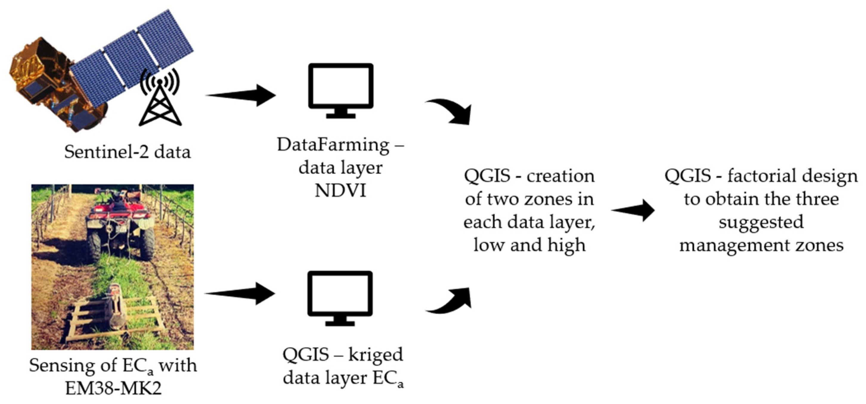
2.2. Remote Measurements
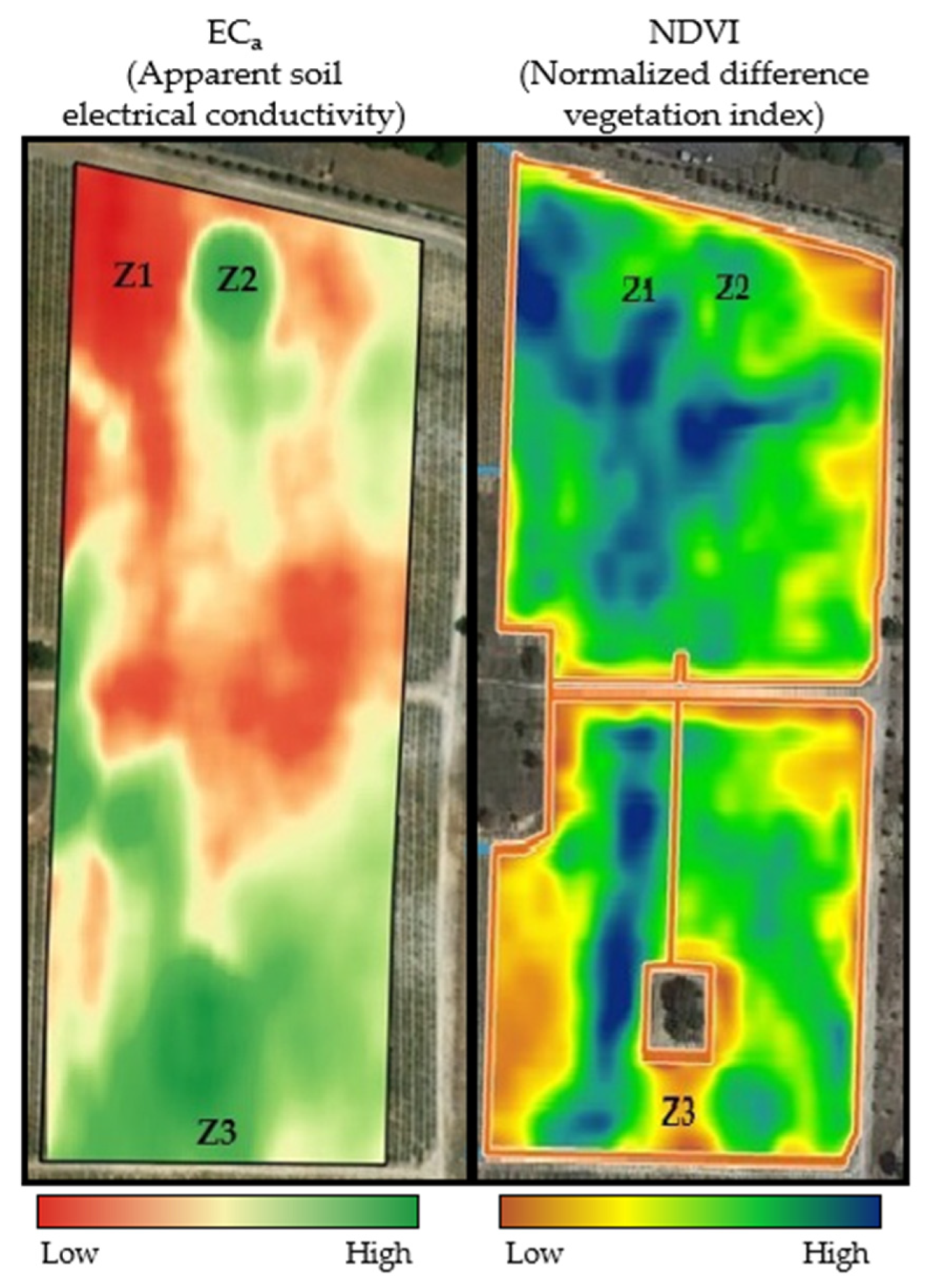
2.2.1. ECa

There are two main methods for measuring ECa: (1) a direct contact method, where electrodes are in direct contact with the soil to inject and measure an electrical current, and (2) an indirect contact method called electromagnetic induction (EMI) where a transmitter coil induces a magnetic field in the soil and a receiver determines the response [16,33].
The ECa map was obtained by the means of an electromagnetic induction (EMI) sensor, the EM38-MK2 sensor [34]. This non-invasive sensor is considered very sensitive in describing the soil sublayer properties, without in-depth disturbance [20].
The sensor was positioned in the vertical dipole with the receiver separated from the transmitter by 1 m [35,36] and was mounted on a four-wheel motorcycle, which passed on every other interrow (intervals of 5.6 m). The ECa sensing data dated from 14 May 2018, and the soil had a water content of about 75% of field capacity during measurement. The data were then kriged in QGIS version 3.16.15 [37], and, using the median values, two levels of ECa were defined: high and low.

2.2.2. NDVI

The expression used to obtain NDVI is extensively described in the literature (e.g., [16,18,38]), where the bands from the near-infrared radiation (NIR) region (from 0.7 to 1.2 µm) and the red radiation region (from 0.6 to 0.7 µm) of the electromagnetic spectrum (EMS) are used for the computation. The indicator varies from +1 to −1, where positive values represent vegetation or high-reflective surfaces, since they have a higher reflectance of NIR radiation, and negative values indicate non-vegetation or senescent and dry vegetation, or clouds or water, as they have a lower reflectance of NIR radiation [38].
The NDVI map used here was obtained with images from the satellite Sentinel-2 [39], from the European Commission’s Copernicus program. The images were downloaded directly through the DataFarming platform [40], which already provided the NDVI map. The image is from tile number T29SMC, which corresponds to continental Portugal. The date was 24 June 2018, a day without clouds, and the images had a resolution of 10 m. In the Sentinel-2 instruments, the bands 8 and 4 correspond to the NIR and red band of the EMS, respectively, and thus are used for NDVI computation. The downloaded images were then treated in QGIS to also obtain two levels of NDVI (also using the median values): high and low.
Also in QGIS, the NDVI map was used in conjunction with the ECa map to obtain, through a factorial design, the three suggested zones, which are combinations of high and low values of NDVI and ECa, as summarized in Figure 1.

2.3. Experimental Design

Within the experimental area, zones were defined based on the low and high levels of two indicators, NDVI and ECa. The experimental design used in the statistical analysis was based on three scenarios: (1) zoning based on NDVI, (2) zoning based on ECa, and (3) zoning based on both indicators, NDVI + ECa.
In the first two scenarios, only two zones were defined: high NDVI (N+) and low NDVI (N−) when using NDVI for zone delineation; high ECa (E+) and low ECa (E−) when using ECa for zone delineation. In the last scenario, three zones were defined as shown in Figure 2: zone one with high levels of NDVI and low of ECa (Z1: N+ E−), zone two with high levels of both NDVI and ECa (Z2: N+ E+), and zone three with low NDVI and high ECa (Z3: N− E+). High and low levels were defined based on the 50 percentile values. In each zone, 3 different plots (replicates) were randomly established. Moreover, in the study area, a zone with low NDVI and low ECa was not detected.

2.4. Soil Analysis

Using a probe, soil samples were collected from the first 0–50 cm of soil. From each plot of each zone, 13 soil samples were taken, making up a total of 117 soil samples (3 zones × 3 plots × 13 samples), that were individually analyzed. Before chemical analysis, the 117 soil samples were air-dried until constant weight and sieved through a 2 mm mesh. The variables assessed in the present study were the following: pH and laboratory-determined soil electrical conductivity (EC1:2), soil organic carbon (SOC), total nitrogen (N), extractable phosphorus (P), exchangeable cations (potassium K+, calcium Ca2+, magnesium Mg2+, and sodium Na+), exchangeable acidity (EA), and effective cation exchange capacity (ECEC).
Soil pH and EC1:2 were measured in a soil:water suspension (p/v) prepared with distilled water, using a 1:2.5 suspension and a potentiometer for pH measurement, and using a 1:2 suspension and an electrical conductivity meter for EC1:2 determination, both measured at room temperature [41]. Furthermore, pH was also measured in a 1:2.5 soil:CaCl2 (0.01 M) suspension [42].
Extractable P was determined using the Égner–Rhiem method and measured through the inductively coupled plasma optical emission spectroscopy (ICP-OES) technique [43]; SOC concentration was determined through the total organic carbon (TOC) method using dry combustion [44]; total N was measured using the micro-Kjeldahl method [45].
Exchangeable cations were determined by extraction with ammonium acetate (1 M at pH 7) and then quantification through the ICP-OES technique; EA was determined through KCl (1 M) extraction, followed by titration with NaOH (0.043475 M); ECEC was determined as the sum of exchangeable cations and EA. The procedures were according to Amacher et al. [46].
Particle size determination was also evaluated in the present work and was determined through the conventional pipette method to obtain the soil percentage of sand, silt, and clay [47].

2.5. Statistical Analysis

The experimental data were analyzed through a one-way variance analysis (ANOVA), using the general linear model procedure to perform the F test with a completely randomized design. Mean separation was performed using the LSD test with the significance level set at α = 0.05. All statistical analyses were performed with the Statistix software package [48]. ANOVA was used in this context to obtain information about the statistical separation between the potential management zones in the study area, as in Li et al. [19].

3. Results and Discussion

3.1. Soil Particle Size

The results of soil particle size analysis from each zone delineated in the three scenarios are shown in Table 1. In zones delineated based on NDVI, the high NDVI levels (N+ zones) are associated with a higher percentage of sand and a lower percentage of clay in the soil, while there are no significant differences for silt. These results indicate that high NDVI is related to soils with more porosity that have better drainage and allow aeration near the root zone, which is important in healthy vine roots [49].
However, when using ECa for zone delineation, high values of the indicator (E+) correspond to a lower percentage of sand and a higher percentage of silt and clay in the soil. This result agrees with other researchers’ work, which demonstrated the positive correlation between soil clay content and ECa, regardless of the soil type or ECa data types [8]. In another study also performed in a vineyard, a negative correlation between EMI-based ECa and soil sand was found [25], similar to the present work findings. The same conclusions were reached by other authors, with the same EM38 sensor [10,13,29,30,31,50], and in a Portuguese vineyard, with the ECa sensor Veris 3150 [51]. Given this positive relationship between ECa and soil clay content, ECa maps can be used for a variety of purposes, such as a base for soil fertilization and irrigation, since clay content is linked to nutrient availability and structural and hydrological properties [51].
In another study, soils with higher clay content had the highest values of NDVI [25]. The authors associated the benefits of soils with a finer texture, specifically having higher water holding capacity, better vegetative vigor, and higher NDVI. However, the results in the present work do not reflect these findings. Quite the opposite, high levels of NDVI were related to low content of clay and high content of sand.
Regarding the scenario NDVI + ECa, the results are equivalent to scenario ECa, where zones with high ECa had significantly less sand in the soil and higher content of clay, regardless of the NDVI levels. It suggests that soil particle size is more related to ECa than to NDVI. Zone delineation using ECa as a proxy should be adequate, as the addition of NDVI did not bring any added value, as already concluded by other researchers [27].

3.2. Soil pH, EC, SOC, N, and P

3.2.1. Soil pH

Values of soil pH (H2O) and pH (CaCl2) showed significant differences between zones, but such variations rely on the scenario considered (Table 2). Using NDVI for zone delineation, only pH (CaCl2) values showed significant differences between zones, while when using ECa, only pH (H2O) showed significant differences. In the NDVI + ECa scenario, the differences between zones are significant, and there is a combination of the above-mentioned results, further evidencing the relationship between pH (H2O) and ECa and between pH (CaCl2) and NDVI.
A positive, and significant, relationship between ECa and pH (H2O) was already observed in other studies [14,51]. Regarding the relationship between NDVI and pH (CaCl2), there is little proof of it; however, using CaCl2 to measure pH is known to be more consistent as it is less affected by environmental changes, i.e., the addition of fertilizer, whereas water extracted pH can vary without changes in exchangeable acidity [52]. As such, in the present work, pH (CaCl2) is well related to NDVI since this measurement method better reflects plant response to pH variations.
Soil pH (H2O) is quite neutral or slightly acidic in the study area, but pH (CaCl2), which should be between 5.5 and 8 for optimum grapevine production [53], is slightly below the minimum threshold when NDVI is high, when ECa is low, and when both are combined. However, pH (CaCl2) is not below five, a threshold associated with stunted shoot and root growth [53].

3.2.2. Soil EC1:2

The low values of laboratory-measured EC1:2 indicate that there are no salinity issues in the soil [41,53]. As can be seen in Table 2, higher values of this variable are related to high ECa, an expected outcome as EC1:2 is a direct measurement of soil salinity, which has a great impact on ECa measurement. This positive correlation was also observed in another study [51]. High EC1:2 is also related to low NDVI, meaning that the high content of exchangeable cations is related to low vegetation health. Low values of NDVI indicate stressed vegetation, with less photosynthetic activity since less near-infrared radiation is reflected [54]. Thus, there might be unbalance in soil nutrient content that is affecting plant nutrition and consequently affecting photosynthetic activity and producing lower values of NDVI.
Additionally, zones with lower values of EC1:2 coincide with zones that have larger particle sizes (higher content of sand), whereas higher values of EC1:2 coincide with smaller particle sizes (higher content of clay), a result also found in the literature [50]. Perhaps the leaching of salts in excess, promoted by the large size of the soil particles in the zone with sandy soil, N+E−, is one of the reasons this zone has a high NDVI. The other zone with a high NDVI, N+E+, is the one with more silt percentage, as seen in Table 1. The EC1:2 in this zone does not significantly differ from EC1:2 in zone N+E−, with both zones having substantially less soil electrical conductivity (EC1:2) in the soil than N−E+, the only zone with a small NDVI. This is another indication that the soil might have an excess of salts, as reported by EC1:2, that is harming crop performance, as reported by the NDVI. However, it remains difficult to assess what has the greatest impact on NDVI: aeration near roots or the leaching of salts, or even the combination of the two.

3.2.3. Soil Organic Carbon (SOC)

SOC content, on the other hand, is very homogeneous within the experimental area since no significant differences are observed between zones, in all scenarios. A similar outcome was obtained in a study performed in a Chilean vineyard, using ECa as an indicator for zone definition [16]. As such, organic matter added to soil, if needed, could be done uniformly across the field. However, since this characteristic is quite temporally stable in the soil, it is not expected to be a necessity in the upcoming years. Even if not observed in the present work, a small correlation between soil organic matter and ECa has been documented in a similar condition, i.e., in a Mediterranean vineyard [51].

3.2.4. Soil Total Nitrogen (Ntot) and Extractable Phosphorus (P)

Concerning Ntot, the results reveal significant differences when using NDVI and NDVI + ECa for zone delineation, but no differences were observed between zones when using only ECa. High NDVI levels were related to a high content of soil Ntot. Here, the importance of NDVI to differentiate management zones for nitrogen fertilization is indisputable, as Ntot strongly influences this indicator. This correlation has been thoroughly studied in the past decades due to the importance of nitrogen to plant biomass production (e.g., recently: [55,56,57]).
Using ECa in the delineation of distinct zones, regarding soil N content, was only effective when used jointly with NDVI. Nevertheless, ECa addition proved to be very effective as the three zones, delineated in the scenario NDVI + ECa, were substantially different from each other and thus can be managed differently.
For extractable P content, the zones were only significantly different when using NDVI for zone definition, with high values of the nutrient being related to high levels of NDVI. In the present work, using ECa for zone definition added no value. The relationship between soil P and the indicators varies in the literature, with some studies finding no significant correlation between ECa and soil P [14,24], whereas other researchers found a significant correlation (R2 = 0.61) between Olsen P and ECa [13]. Serrano et al. [24] found a small connection between P and NDVI (p < 0.05) in a vineyard. By considering the soil type, in terms of soil texture, ECEC, and humic matter, some authors have improved the correlation between this nutrient (and others) and ECa [58].

3.3. Cation Exchange Complex

3.3.1. Exchangeable Cations

The exchangeable cation content is significantly different between zones in all three scenarios, as seen in Table 3. The high content of exchangeable cations is related to low NDVI and to high ECa in the scenarios where only one indicator is used. This finding corroborates the hypothesis mentioned in Section 3.2.2., which stated that low vegetation health (low NDVI) may be related to a high content of salts in the soil. Aeration promoted by the larger particle soil also plays an important role in plant health; however, these results do indicate that leaching of excess salts in these soils may have a greater impact on crop health and NDVI than the aeration.
In the results from scenario NDVI + ECa, the effect of K+ on ECa is noticeable, since high K+ content is related to high ECa, regardless of NDVI levels. This result is not in agreement with other results, as some have found no correlation between ECa and K+ [14,50]. A similar but inverse relationship was observed between Ca2+ and NDVI in the present work, with low Ca2+ related to high NDVI levels.
Concerning Mg2+ and Na+, both differed at the highest significance level in all three scenarios: NDVI, ECa, and NDVI + ECa. Both cations are normally correlated with ECa, but Na+ has shown a more dominant correlation with ECa in previous studies [14,50] as compared to the present results. In another study, Mg2+ was the most correlated cation with ECa, and since it was most correlated at higher depth, the authors justified this correlation with the parent material of the soil [13]. In the present case study, both Na+ and Mg2+ were also highly related to NDVI.
Additionally, the soil content of Mg2+ is significantly different between the three zones established in the NDVI + ECa scenario. This is a very positive outcome because delineating zones based on two indicators, instead of just one, allowed the definition of three significantly distinct zones in terms of Mg2+, which in turn, if managed differently, allows for better soil and crop fertilization, more adequate to the field intra-variability.

3.3.2. Exchangeable Acidity (EA) and Effective Cation Exchange Capacity (ECEC)

EA differed between zones delineated with ECa, with high ECa associated with high EA, but it did not differ when using NDVI. However, in the scenario NDVI + ECa, the three zones were significantly different from each other, again showing the effectiveness of combining two indicators for the delineation of management zones. The differences observed in EA results are the same as the differences obtained in pH (H2O) results, implying that EA is positively related to distilled water extracted pH, rather than calcium chloride extracted pH. Contrarily to what was previously mentioned, the variations in pH (H2O) accompanied the EA variations in the present work conditions. The low values of EA imply that no acidity issues are expected in the soil [59].
As for ECEC, due to the content of exchangeable cations and EA, high values of ECEC correspond to low NDVI and high ECa. Regarding ECEC, the differences between zones, and the relationship with NDVI and ECa, are the same as those obtained for soil clay content. This result is similar to those reported in previous works [8,13,14], evidencing the influence of soil clay content on ECa measurement [58]. This agrees with the rationale that ECa increases with the increase in charges in the soil surfaces, e.g., an increase in clay minerals in the soil matrix, and an increase in exchangeable cations [13].
Like soil Mg2+, ECEC content is substantially different between the three established zones (in scenario NDVI + ECa), suggesting a strong influence of the nutrient in ECEC.

3.4. Ratios within the Cation Exchange Complex

The ratios between cations and the percentages of the cations within ECEC are presented in Table 4. The understanding of the exchangeable cation content in soil is very important, as they are in a plant-available form and consequently important for plant growth [13]. Equally important are the cation ratios in the soil cation exchange complex, as a disequilibrium between cation content may affect soil physical properties, such as clay dispersion due to Na excess, and nutrient availability to plants, as the excess of one cation may harm another cation’s absorption (e.g., potassium and magnesium antagonism), therefore affecting root growth and development and plant performance and productivity.
As seen, high NDVI and low ECa are related to higher values of Ca2+/ECEC and K+/ECEC and lower proportions of Mg2+/ECEC and Na+/ECEC. Hence, it is natural that they are also related to higher Ca2+/Mg2+ and K+/Mg2+ ratios.
In the scenario where both indicators are used for zone delineation, almost all ratios, except for K+/ECEC and Na+/ECEC, were significantly different between the three zones, again demonstrating the usefulness and effectiveness of using two indicators for zone delineation, one for soil salinity and a multitude of soil chemical and physical parameters (ECa), and another that relates to crop response and health (NDVI).
The Ca2+/Mg2+ ratio, which is important as it indicates the likely effect of clay dispersion consequent from Mg2+ excess [60], should be within the interval 2–10 for optimal vineyard production [53]. However, the ratio in zone N−, zone E+, and zone N−E+ is below the mentioned interval, which may indicate an excess of Mg2+ in relation to Ca2+, in turn inducing clay dispersion and affecting soil structural stability. Lanyon et al. [53] suggested that this effect is induced in soils with ratios of Ca2+/Mg2+ below 1. This is not seen in the results; however, zones N− and N−E+ have this ratio very close to 1 (1.01 as seen in Table 4). Therefore, this is something to investigate in the future as the excess of Mg2+ may cause soil damage and, consequently, loss of crop productivity.
Simultaneously, the K+/Mg2+ ratio, which should be between 0.1 and 0.4 for optimal vine production [53], is below the minimum threshold in two of the same zones: N− and N−E+, reinforcing the hypothesis of excess Mg2+ and the existence of an ionic imbalance in the soil’s chemical composition. The fact that the excess of Mg2+ happens in zones with high ECa and low NDVI suggests that the high content of this cation is increasing soil cation concentration to a point of decreasing crop vegetation health status and, eventually, affecting crop production.
Indeed, the ratio of Mg2+/ECEC is very high in these zones (30 is the maximum value for this ratio according to Lanyon et al. [53]), confirming the excess of Mg2+ in this case study. According to the same author, Ca2+/ECEC, K+/ECEC, and Na+/ECEC have reference values for optimal grape production (Table 4), and as seen in the results, the zones with the Mg2+ disequilibrium fail to be within these intervals: Ca2+ is below as well as K+, but Na+ is slightly above. An excess of Na+ may even aggravate clay dispersion in these zones. The unhealthy vegetation, as reported by the low NDVI, may also be due to ion antagonism as the excess of Mg2+ is injuring K+ absorption. This problem can be solved by lowering pH to make the absorption of Mg2+ difficult, but a more successful approach is potassium fertilization [61]. The success rate does depend on various factors, such as soil lime content [62].
Thereby, the zones with high ECa and low NDVI deserve special attention, in the matter of fertilization purposes. Furthermore, throughout the present work, the results point to a negative relationship between ECa and NDVI, since the differences obtained between zones are somewhat opposite when using one or the other indicator, i.e., one variable is high with high levels of ECa and low levels of NDVI. This often happens in the results, with most of the soil variables tackled in the world, which supports the idea that, in the present case, a high concentration of exchangeable cations (more precisely, Mg2+) is related to low plant vigor. In a Bordeaux vineyard, this relation was positive rather than negative [25], and in an arid environment, the relationship was also negative, which was attributed to salinity [18].
The interpretation of soil analysis relative to crop yield prediction is very uncertain in a vineyard since it is a perennial plant with storage organs that temporally varies in nutrient content [53]. Nonetheless, the present soil evaluation whilst using two remote indicators (NDVI and ECa) for soil sampling proved to be extremely important because it allowed the definition of different zones, with contrasting soil properties in the study area.

4. Conclusions

For a few of the soil variables, NDVI alone was sufficient to delineate different zones, e.g., pH (CaCl2) and extractable P. For other soil variables, such as pH (H2O), ECa allowed an effective zone definition. However, for most of the soil variable content, the combined use of the indicators proved to be more effective, as the three delineated zones in scenario NDVI + ECa were significantly distinct, allowing the three zones to be managed differently, which would have not been possible if only one indicator had been used. That is the case of soil Ntot, Mg2+, EA, and ECEC and the ratios Ca2+/Mg2+, K+/Mg2+, Ca2+/ECEC, and Mg2+/ECEC. As such, it is concluded that the use of both indicators, NDVI and ECa, is more beneficial than using just one and that there is a high potential for differential application of crop nutrients and soil management in the present vineyard.
It is also formulated that, in the present study conditions, plant health is related to sand content because it allowed the leaching of excess salts, in this case, excess of Mg2+. The negative relationship between NDVI and ECa (the latter impacted by the excess of Mg2+) also corroborates this hypothesis. However, further analysis is needed, such as petiole analysis at flowering and veraison stage, and registration of grape production is also important.
If the soil characterization had been performed as if the 6.77 ha of vineyard were homogenous, as is conventionally done, this ionic problem would have not been identified and would remain uncorrected. Hence, the use of these technological tools, namely NDVI and ECa, is of great relevance in today’s context and if used properly, is capable of increasing food production with less environmental impact.
Nevertheless, validation of these results in other conditions, with different soil types or in different regions, is still needed.

Author Contributions

Conceptualization, R.P.B. and H.R.; Data curation, C.E., R.P.B., H.R. and M.M.; Funding acquisition, D.F.; Investigation, C.E.; Supervision, H.R.; Writing—original draft, C.E.; Writing—review and editing, D.F., R.P.B., M.B. and H.R. All authors have read and agreed to the published version of the manuscript.

Funding

This research was funded by (1) the Project Nutri2Cycle: H2020-SFS-30-2017 “Transition towards a more carbon and nutrient efficient agriculture in Europe”, funded by the European Union, Program Horizon 2020 (Grant Agreement No. 773682); (2) national funds through FCT—Fundação para a Ciência e a Tecnologia, I.P., in the scope of the project Linking Landscape, Environment, Agriculture and Food Research Centre Ref. UIDB/04129/2020 and UIDP/04129/2020. This document reflects only the authors’ view, and the Union is not liable for any use that may be made of the information contained therein.

Acknowledgments

Many thanks to the José Maria da Fonseca company (https://www.jmf.pt/, accessed on 24 March 2022), which provided the study area that made the present work possible. We also appreciate their help and time.

Conflicts of Interest

The authors declare no conflict of interest. The funders had no role in the design of the study; in the collection, analyses, or interpretation of data; in the writing of the manuscript, or in the decision to publish the results.

References

  1. Van Alphen, B.J.; Stoorvogel, J.J. A methodology for precision nitrogen fertilization in high-input farming systems. Precis. Agric. 2000, 2, 319–332. [Google Scholar] [CrossRef]
  2. Balafoutis, A.; Beck, B.; Fountas, S.; Vangeyte, J.; Van Der Wal, T.; Soto, I.; Gómez-Barbero, M.; Barnes, A.; Eory, V. Precision agriculture technologies positively contributing to ghg emissions mitigation, farm productivity and economics. Sustainability 2017, 9, 1339. [Google Scholar] [CrossRef] [Green Version]
  3. Bramley, R.G.V.; Lamb, D.W. Making sense of vineyard variability in Australia. In Precision Viticulture, Proceedings of an International Symposium Held as Part of the IX Congreso Latinoamericano de Viticultura y Enologia, Chile; Ortega, R., Esser, A., Eds.; Centro de Agricultura de Precisión, Facultad de Agronomía e Ingenería Forestal, Pontificia Universidad Católica de Chile: Santiago, Chile, 2003; pp. 35–54. [Google Scholar]
  4. Du, Q.; Chang, N.B.; Yang, C.; Srilakshmi, K.R. Combination of multispectral remote sensing, variable rate technology and environmental modeling for citrus pest management. J. Environ. Manag. 2008, 86, 14–26. [Google Scholar] [CrossRef] [PubMed]
  5. Leroux, C.; Tisseyre, B. How to measure and report within-field variability: A review of common indicators and their sensitivity. Precis. Agric. 2019, 20, 562–590. [Google Scholar] [CrossRef]
  6. Brevik, E.C.; Fenton, T.E.; Lazari, A. Soil electrical conductivity as a function of soil water content and implications for soil mapping. Precis. Agric. 2006, 7, 393–404. [Google Scholar] [CrossRef]
  7. Carroll, Z.L.; Oliver, M.A. Exploring the spatial relations between soil physical properties and apparent electrical conductivity. Geoderma 2005, 128, 354–374. [Google Scholar] [CrossRef]
  8. Sudduth, K.A.; Kitchen, N.R.; Wiebold, W.J.; Batchelor, W.D.; Bollero, G.A.; Bullock, D.G.; Clay, D.E.; Palm, H.L.; Pierce, F.J.; Schuler, R.T.; et al. Relating apparent electrical conductivity to soil properties across the north-central USA. Comput. Electron. Agric. 2005, 46, 263–283. [Google Scholar] [CrossRef]
  9. Jung, W.K.; Kitchen, N.R.; Sudduth, K.A.; Kremer, R.J.; Motavalli, P.P. Relationship of Apparent Soil Electrical Conductivity to Claypan Soil Properties. Soil Sci. Soc. Am. J. 2005, 69, 883–892. [Google Scholar] [CrossRef] [Green Version]
  10. Stepień, M.; Samborski, S.; Gozdowski, D.; Dobers, E.S.; Chormański, J.; Szatylowicz, J. Assessment of soil texture class on agricultural fields using ECa, Amber NDVI, and topographic properties. J. Plant Nutr. Soil Sci. 2015, 178, 523–536. [Google Scholar] [CrossRef]
  11. Domsch, H.; Giebel, A. Estimation of Soil Textural Features from Soil Electrical Conductivity Recorded Using the EM38. Precis. Agric. 2004, 5, 389–409. [Google Scholar] [CrossRef]
  12. Dunn, B.W.; Beecher, H.G. Using electro-magnetic induction technology to identify sampling sites for soil acidity assessment and to determine spatial variability of soil acidity in rice fields. Aust. J. Exp. Agric. 2007, 47, 208–214. [Google Scholar] [CrossRef]
  13. Hedley, C.B.; Yule, I.J.; Eastwood, C.R.; Shepherd, T.G.; Arnold, G. Rapid identification of soil textural and management zones using electromagnetic induction sensing of soils. Soil Res. 2004, 42, 389–400. [Google Scholar] [CrossRef]
  14. Peralta, N.R.; Costa, J.L. Delineation of management zones with soil apparent electrical conductivity to improve nutrient management. Comput. Electron. Agric. 2013, 99, 218–226. [Google Scholar] [CrossRef] [Green Version]
  15. Corwin, D.L.; Lesch, S.M. Apparent soil electrical conductivity measurements in agriculture. Comput. Electron. Agric. 2005, 46, 11–43. [Google Scholar] [CrossRef]
  16. Ortega-Blu, R.; Molina-Roco, M. Evaluation of vegetation indices and apparent soil electrical conductivity for site-specific vineyard management in Chile. Precis. Agric. 2016, 17, 434–450. [Google Scholar] [CrossRef]
  17. Verhulst, N.; Govaerts, B.; Sayre, K.D.; Deckers, J.; François, I.M.; Dendooven, L. Using NDVI and soil quality analysis to assess influence of agronomic management on within-plot spatial variability and factors limiting production. Plant Soil 2009, 317, 41–59. [Google Scholar] [CrossRef]
  18. Aldakheel, Y.Y. Assessing NDVI Spatial Pattern as Related to Irrigation and Soil Salinity Management in Al-Hassa Oasis, Saudi Arabia. J. Indian Soc. Remote Sens. 2011, 39, 171–180. [Google Scholar] [CrossRef]
  19. Li, Y.; Shi, Z.; Wu, C.F.; Li, H.Y.; Li, F. Determination of potential management zones from soil electrical conductivity, yield and crop data. J. Zhejiang Univ. Sci. B 2008, 9, 68–76. [Google Scholar] [CrossRef] [Green Version]
  20. Andrenelli, M.C.; Magini, S.; Pellegrini, S.; Perria, R.; Vignozzi, N.; Costantini, E.A.C. The use of the ARP© system to reduce the costs of soil survey for precision viticulture. J. Appl. Geophys. 2013, 99, 24–34. [Google Scholar] [CrossRef]
  21. Bonilla, I.; De Toda, F.M.; Martínez-Casasnovas, J.A. Vineyard zonal management for grape quality assessment by combining airborne remote sensed imagery and soil sensors. Remote Sens. Agric. Ecosyst. Hydrol. XVI 2014, 9239, 92390S. [Google Scholar] [CrossRef]
  22. Botelho, M.; Cruz, A.; Mourato, C.; Castelo-Branco, J.; Ricardo-da-Silva, J.; Castro, R.; Ribeiro, H.; Braga, R. Variable-rate mechanical pruning: A new way to prune vines. Acta Hortic. 2021, 1314, 307–312. [Google Scholar] [CrossRef]
  23. Tagarakis, A.; Liakos, V.; Fountas, S.; Koundouras, S.; Gemtos, T.A. Management zones delineation using fuzzy clustering techniques in grapevines. Precis. Agric. 2013, 14, 18–39. [Google Scholar] [CrossRef]
  24. Serrano, J.; Da Silva, J.M.; Shahidian, S.; Silva, L.L.; Sousa, A.; Baptista, F. Differential vineyard fertilizer management based on nutrient’s spatio-temporal variability. J. Soil Sci. Plant Nutr. 2017, 17, 46–61. [Google Scholar]
  25. Hubbard, S.S.; Schmutz, M.; Balde, A.; Falco, N.; Peruzzo, L.; Dafflon, B.; Léger, E.; Wu, Y. Estimation of soil classes and their relationship to grapevine vigor in a Bordeaux vineyard: Advancing the practical joint use of electromagnetic induction (EMI) and NDVI datasets for precision viticulture. Precis. Agric. 2021, 22, 1353–1376. [Google Scholar] [CrossRef]
  26. Sams, B.; Bramley, R.G.V.; Sanchez, L.; Dokoozlian, N.; Ford, C.; Pagay, V. Remote Sensing, Yield, Physical Characteristics, and Fruit Composition Variability in Cabernet Sauvignon Vineyards. Am. J. Enol. Vitic. 2022, 73, 93–105. [Google Scholar] [CrossRef]
  27. von Hebel, C.; Reynaert, S.; Pauly, K.; Janssens, P.; Piccard, I.; Vanderborght, J.; van der Kruk, J.; Vereecken, H.; Garré, S. Toward high-resolution agronomic soil information and management zones delineated by ground-based electromagnetic induction and aerial drone data. Vadose Zone J. 2021, 20, 1539–1663. [Google Scholar] [CrossRef]
  28. Uribeetxebarria, A.; Martínez-Casasnovas, J.A.; Escolà, A.; Rosell-Polo, J.R.; Arnó, J. Stratified sampling in fruit orchards using cluster-based ancillary information maps: A comparative analysis to improve yield and quality estimates. Precis. Agric. 2019, 20, 179–192. [Google Scholar] [CrossRef] [Green Version]
  29. Millán, S.; Moral, F.J.; Prieto, M.H.; Pérez-Rodríguez, J.M.; Campillo, C. Mapping soil properties and delineating management zones based on electrical conductivity in a hedgerow olive grove. Trans. ASABE 2019, 62, 749–760. [Google Scholar] [CrossRef]
  30. Esteves, C.; Fangueiro, D.; Ribeiro, H.; Braga, R. Remote sensing (NDVI) and Apparent soil electrical conductivity (ECap) to delineate different zones in a vineyard. Biol. Life Sci. Forum 2021, 3, 42. [Google Scholar] [CrossRef]
  31. WRB-IUSS. World Reference Base for Soil Resources. World Soil Resources Reports 106. World Soil Resources Reports; No. 106; FAO: Rome, Italy, 2015. [Google Scholar]
  32. Instituto Português da Atmosfera e do Mar. Available online: https://www.ipma.pt/pt/oclima/normais.clima/ (accessed on 27 March 2021).
  33. Singh, G.; Williard, K.W.J.; Schoonover, J.E. Spatial relation of apparent soil electrical conductivity with crop yields and soil properties at different topographic positions in a small agricultural watershed. Agronomy 2016, 6, 57. [Google Scholar] [CrossRef] [Green Version]
  34. Geonics Limited. Available online: http://www.geonics.com/html/em38.html (accessed on 27 March 2021).
  35. Heil, K.; Schmidhalter, U. Comparison of the EM38 and EM38-MK2 electromagnetic induction-based sensors for spatial soil analysis at field scale. Comput. Electron. Agric. 2015, 110, 267–280. [Google Scholar] [CrossRef]
  36. Heil, K.; Schmidhalter, U. The application of EM38: Determination of soil parameters, selection of soil sampling points and use in agriculture and archaeology. Sensors 2017, 17, 2540. [Google Scholar] [CrossRef] [PubMed] [Green Version]
  37. QGIS Version 3.16.15. QGIS Geographic Information System. QGIS Association. Available online: http://www.qgis.org (accessed on 21 March 2022).
  38. Bhunia, G.S.; Shit, P.K.; Pourghasemi, H.R. Soil organic carbon mapping using remote sensing techniques and multivariate regression model. Geocarto Int. 2017, 34, 215–226. [Google Scholar] [CrossRef]
  39. Copernicus Sentinel-2. Available online: https://sentinel.esa.int/web/sentinel/missions/sentinel-2 (accessed on 15 April 2021).
  40. DataFarming. Data Farming-High Resolution Images Available Now. DataFarming. Available online: https://www.datafarming.com.au/ (accessed on 21 March 2022).
  41. Sonmez, S.; Buyuktas, D.; Okturen, F.; Citak, S. Assessment of different soil to water ratios (1:1, 1:2.5, 1:5) in soil salinity studies. Geoderma 2008, 144, 361–369. [Google Scholar] [CrossRef]
  42. Fotyma, M.; Jadczyszyn, T.; Jozefaciuk, G. Hundredth molar calcium chloride extraction procedure. Part II: Calibration with conventional soil testing methods for pH. Commun. Soil Sci. Plant Anal. 1998, 29, 1625–1632. [Google Scholar] [CrossRef]
  43. Egnér, H.; Riehm, H.; Domingo, W.R. Investigations on chemical soil analysis as a basis for assessing the nutrient status of soils. II. Chemical Extraction Methods for Phosphorus and Potassium Determination. K. Lantbr. Ann. 1960, 26, 199–215. [Google Scholar]
  44. Nelson, D.W.; Sommers, L.E. Total Carbon, Organic Carbon, and Organic Matter. In Methods of Soil Analysis: Part 2 Chemical and Microbiological Properties 9.2.2, 2nd ed.; The American Society of Agronomy, Inc.: Madison, WI, USA; Soil Science Society of America, Inc.: Madison, WI, USA, 1996; Chapter 29. [Google Scholar] [CrossRef]
  45. Bremner, J.M. Determination of nitrogen in soil by the Kjeldahl method. J. Agric. Sci. 1960, 55, 11–33. [Google Scholar] [CrossRef]
  46. Amacher, M.C.; Henderson, R.E.; Breithaupt, M.D.; Seale, C.L.; LaBauve, J.M. Unbuffered and Buffered Salt Methods for Exchangeable Cations and Effective Cation-Exchange Capacity. Soil Sci. Soc. Am. J. 1990, 54, 1036–1042. [Google Scholar] [CrossRef]
  47. Gee, G.W.; Bauder, J.W. Particle-size Analysis. In Methods of Soil Analysis: Part I—Physical and Mineralogical Methods; Campbell, G.S., Jackson, R.D., Mortland, M.M., Nielsen, D.R., Klute, A., Eds.; American Society of Agronomy: Madison, WI, USA, 1986; pp. 383–411. [Google Scholar]
  48. Statistix Program Version 9.0; Analytical Software, Tallahassee, FL, USA. Free Trial. Available online: https://www.statistix.com/ (accessed on 27 March 2021).
  49. Stevens, R.M.; Douglas, T. Distribution of grapevine roots and salt under drip and full-ground cover microjet irrigation systems. Irrig. Sci. 1994, 15, 147–152. [Google Scholar] [CrossRef]
  50. Rodríguez-Pérez, J.R.; Plant, R.E.; Lambert, J.J.; Smart, D.R. Using apparent soil electrical conductivity (ECa) to characterize vineyard soils of high clay content. Precis. Agric. 2011, 12, 775–794. [Google Scholar] [CrossRef] [Green Version]
  51. Serrano, J.; da Silva, J.; Shahidian, S.; Silva, L.; Sousa, A.; Baptista, F. Spatial variability of soil phosphorus, potassium and pH: Evaluation of the potential for improving vineyard fertilizer management. In Precision Agriculture’15; Stafford, J.V., Ed.; Wageningen Academic Publishers: Wageningen, The Netherlands, 2015; pp. 495–502. [Google Scholar] [CrossRef]
  52. Kissel, D.E.; Sonon, L.; Vendrell, P.F.; Isaac, R.A. Salt concentration and measurement of soil pH. Commun. Soil Sci. Plant Anal. 2009, 40, 179–187. [Google Scholar] [CrossRef]
  53. Lanyon, D.M.; Cass, A.; Hasen, D. The Effect of Soil Properties on Vine Performance. 2004. Available online: https://www.researchgate.net/publication/228433458 (accessed on 27 March 2022).
  54. Hall, A.; Lamb, D.W.; Holzapfel, B.; Louis, J. Optical remote sensing applications in viticulture—A review. Aust. J. Grape Wine Res. 2002, 8, 36–47. [Google Scholar] [CrossRef]
  55. Peri, P.L.; Rosas, Y.M.; Ladd, B.; Toledo, S.; Lasagno, R.G.; Pastur, G.M. Modeling soil nitrogen content in south Patagonia across a climate gradient, vegetation type, and grazing. Sustainability 2019, 11, 2707. [Google Scholar] [CrossRef] [Green Version]
  56. Wang, S.; Zhuang, Q.; Jin, X.; Yang, Z.; Liu, H. Predicting soil organic carbon and soil nitrogen stocks in topsoil of forest ecosystems in Northeastern China using remote sensing data. Remote Sens. 2020, 12, 1115. [Google Scholar] [CrossRef] [Green Version]
  57. Zhang, J.; Wei, Q.; Xiong, S.; Shi, L.; Ma, X.; Du, P.; Guo, J. A spectral parameter for the estimation of soil total nitrogen and nitrate nitrogen of winter wheat growth period. Soil Use Manag. 2021, 37, 698–711. [Google Scholar] [CrossRef]
  58. Heiniger, R.W.; Mcbride, R.G.; Clay, D.E. Using Soil Electrical Conductivity to Improve Nutrient Management. Agron. J. 2003, 95, 508–519. [Google Scholar] [CrossRef]
  59. Dai, Z.; Liu, Y.; Wang, X.; Zhao, D. Changes in pH, CEC and exchangeable acidity of some forest soils in southern China during the last 32–35 years. Water Air Soil Pollut. 1998, 108, 377–390. [Google Scholar] [CrossRef]
  60. Bennett, J.M.L.; Marchuk, A.; Marchuk, S. An alternative index to the exchangeable sodium percentage for an explanation of dispersion occurring in soils. Soil Res. 2016, 54, 949–957. [Google Scholar] [CrossRef]
  61. Michael Hannan, J.; Michael, J. Potassium-Magnesium Antagonism in High Magnesium Vineyard Soils Recommended Citation. Master’s Thesis, Iowa State University, Ames, IA, USA, 2011. [Google Scholar]
  62. Gluhić, D.; Ćustić, M.H.; Petek, M.; Čoga, L.; Slunjski, S.; Sinčić, M. The Content of Mg, K and Ca Ions in Vine Leaf under Foliar Application of Magnesium on Calcareous Soils. Agric. Conspec. Sci. 2009, 74, 81–84. [Google Scholar]
Figure 1. Summary of the procedures performed to obtain the ECa map, the NDVI map, and the map with the three distinct zones in terms of these two indicators.
Agronomy 12 01331 g001
Figure 2. Satellite image of the study area (6.77 ha), with ECa and NDVI maps and the respective legend. In the figure, it is also possible to view the three delineated zones (Z1, Z2, and Z3 as mentioned in [30]).
Agronomy 12 01331 g002
Table 1. Mean values of soil percentage of sand, silt, and clay according to zone and indicator used.
Zone DesignSandSiltClay
%
NDVI
N+79.25 a7.1413.61 b
N−71.16 b6.6722.17 a
Signif.*ns**
ECa
E+72.29 b7.62 a20.09 a
E−85.06 a5.71 b9.23 b
Signif.*******
NDVI + ECa
N+ E−85.06 a5.71 b9.23 b
N+ E+73.43 b8.58 a18.00 a
N− E+71.16 b6.67 b22.17 a
Signif.********
Signif.—significance level by the F test, ns—non-significant at p < 0.05 level, significant at p < 0.05 (*), p < 0.01 (**), and p < 0.001 (***) by the F test. In each column, values followed by the same letter do not significantly differ by the LSD test at α = 0.05.
Table 2. Mean values of soil pH (extracted with H2O and CaCl2), electrical conductivity (1:2 soil:water extraction), soil organic carbon (SOC), total nitrogen (Ntot), and extractable phosphorus (P) according to zone and indicator used.
Zone DesignpHpHEC1:2SOCNtotExtractable P
(H2O)(CaCl2)(µS cm−1)(%)(mg kg−1)(mg kg−1)
NDVI
N+6.375.35 b72.86 b0.42285.64 a19.20 a
N−6.515.70 a161.27 a0.42179.85 b8.83 b
Signif.ns******ns****
ECa
E+6.49 a5.52121.19 a0.42247.9113.69
E−6.25 b5.3664.60 b0.42255.3019.85
Signif.**ns***nsnsns
NDVI + ECa
N+ E−6.25 b5.36 b64.60 b0.42255.30 b19.85
N+ E+6.48 a5.35 b81.11 b0.42315.98 a18.55
N− E+6.51 a5.70 a161.27 a0.42179.85 c8.83
Signif.********ns***ns
Signif.—significance level by the F test, ns—non-significant at p < 0.05 level, significant at p < 0.05 (*), p < 0.01 (**), and p < 0.001 (***) by the F test. In each column, values followed by the same letter do not significantly differ by the LSD test at α = 0.05.
Table 3. Mean values of soil exchangeable cations, exchangeable acidity (EA), and effective cation exchange capacity (ECEC) according to zone and indicator used.
Zone DesignExchangeable CationsEAECEC
K+Ca2+Mg2+Na+
(cmol+ kg−1)
NDVI
N+0.19 b1.83 b0.76 b0.07 b0.223.07 b
N−0.23 a3.03 a2.96 a0.43 a0.226.87 a
Signif.**********ns***
ECa
E+0.23 a2.52 a2.01 a0.26 a0.28 a5.31 a
E−0.15 b1.66 b0.45 b0.04 b0.11 b2.40 b
Signif.*****************
NDVI + ECa
N+ E−0.15 b1.66 b0.45 c0.04 b0.11 c2.40 c
N+ E+0.23 a2.01 b1.07 b0.09 b0.33 a3.74 b
N− E+0.23 a3.03 a2.96 a0.43 a0.22 b6.87 a
Signif.******************
Signif.—significance level by the F test, ns—non-significant at p < 0.05 level, significant at p < 0.05 (*), p < 0.01 (**), and p < 0.001 (***) by the F test. In each column, values followed by the same letter do not significantly differ by the LSD test at α = 0.05.
Table 4. Mean values of ratios between Ca2+ and Mg2+ and K+ and Mg2+ and percentages of the cations within the effective cation exchange capacity (ECEC) according to zone and indicator used. Also shown are the “suggested criteria for soil chemical status for sustainable vine health for wine grape production” [53].
Zone DesignCa2+/Mg2+K+/Mg2+Ca2+/ECECK+/ECECMg2+/ECECNa+/ECEC
%
NDVI
N+3.18 a0.32 a61.41 a6.41 a22.31 b2.13 b
N−1.01 b0.08 b41.99 b3.59 b44.56 a6.22 a
Signif.******************
ECa
E+1.62 b0.17 b48.32 b4.95 b35.59 a4.35 a
E−4.12 a0.38 a68.17 a6.51 a18.01 b1.78 b
Signif.******************
NDVI + ECa
N+ E−4.12 a0.38 a68.17 a6.51 a18.01 c1.78 b
N+ E+2.24 b0.25 b54.65 b6.31 a26.61 b2.48 b
N− E+1.01 c0.08 c41.99 c3.59 b44.56 a6.22 a
Signif.******************
Reference values according to
Lanyon et al. [53]
2–100.1–0.460–805–1015–30<6
Signif.—significance level by the F test, significant at p < 0.001 (***) by the F test. In each column, values followed by the same letter do not significantly differ by the LSD test at α = 0.05.
Publisher’s Note: MDPI stays neutral with regard to jurisdictional claims in published maps and institutional affiliations.

