
Hyperspectral Sensing of Plant Diseases: Principle and Methods


1
College of Engineering and Technology, Southwest University, Chongqing 400715, China
2
Key Laboratory of Modern Agricultural Equipment and Technology (Jiangsu University), Ministry of Education, School of Agricultural Engineering, Jiangsu University, Zhenjiang 212013, China
3
Interdisciplinary Research Center for Agriculture Green Development in Yangtze River Basin, Southwest University, Chongqing 400715, China
4
Institute of Urban Agriculture, Chinese Academy of Agricultural Sciences, Chengdu 610213, China
*
Authors to whom correspondence should be addressed.
†
These authors contributed equally to this work.
Agronomy 2022, 12(6), 1451; https://0-doi-org.brum.beds.ac.uk/10.3390/agronomy12061451
Submission received: 7 April 2022
/
Revised: 13 June 2022
/
Accepted: 13 June 2022
/
Published: 17 June 2022
(This article belongs to the Special Issue Agricultural Environment and Intelligent Plant Protection Equipment)
Abstract
:Pathogen infection has greatly reduced crop production. As the symptoms of diseases usually appear when the plants are infected severely, rapid identification approaches are required to monitor plant diseases at early the infection stage and optimize control strategies. Hyperspectral imaging, as a fast and nondestructive sensing technology, has achieved remarkable results in plant disease identification. Various models have been developed for disease identification in different plants such as arable crops, vegetables, fruit trees, etc. In these models, important algorithms, such as the vegetation index and machine learning classification and methods have played significant roles in the detection and early warning of disease. In this paper, the principle of hyperspectral imaging technology and common spectral characteristics of plant disease symptoms are discussed. We reviewed the impact mechanism of pathogen infection on the photo response and spectrum features of the plants, the data processing tools and algorithms of the hyperspectral information of pathogen-infected plants, and the application prospect of hyperspectral imaging technology for the identification of plant diseases.
1. Introduction
Pathogens have brought great challenges to crop production in the last two decades. The reduction of crop yield induced by plant diseases can be up to 28.1% for wheat, 40.9% for rice, 41.4% for maize, 21% for potato, and 32.4% for soybean [1]. Several reasons may contribute to the increase in incidence around the world. Firstly, the globalization of human activities is promoting a more rapid spread and wider distribution of plant pathogens [2]. Secondly, commercialized high-yield varieties are bred from genotypes that are cultivated in certain regions. These varieties may not be adapted to new regional environments and may be less resistant to the local plant pathogens compared to their native wild relatives [3]. Finally, heavy fertilizer application, the large-scale cultivation of monocultures, and reduced crop rotation impact the soil bacterial composition and damage disease-suppressive microorganisms. As a result, there might be a higher possibility for the plants to be infected by pathogens [4].
Conventionally, plant diseases are identified visually according to symptoms when plants are infected severely by pathogens. This is usually quite time-consuming and labor-intensive. Furtherly, it is also a drawback for crop protection with fungicide application, as a better control effect could occur when spraying is conducted at the early stage of pathogen infection. In addition to manual monitoring, biological and molecular detection approaches also provide accurate assessment results of plant diseases. However, a laboratory bioassay can have a high cost and poor real-time performance as well as a limited sample size, which will restrict the measurement scale [5,6,7]. Thus, it is of great significance to evaluate the occurrence of plant diseases and provide an early warning of pathogen infection in crops in time. To satisfy the requirements of the high-throughput detection of plant diseases for precise fungi control, non-destructive and automatic remote detection methods with high sensitivity and reliability are required.
In recent years, modern sensing technologies have been applied for the automatic detection and early warning of plant diseases [8]. For instance, the infrared thermal imaging system has been applied to identify tomato mosaic virus and wheat leaf rust [9]; chlorophyll fluorescence imaging technology was applied to monitor the photosynthetic fingerprint of citrus Huanglongbing [10]; the deep learning model significantly improved the classification accuracy and efficiency of RGB images of healthy or pathogen-infected plants. However, the machine vision technology could only identify plant diseases if the symptoms were obviously apparent on the plant leaves, when it was usually too late for fungicide application. Compared to other sensing approaches, spectral imaging technology has been applied most commonly and has presented remarkable application potential in the real-time detection and evaluation of plant diseases [11,12,13]. In this review, we summarize the principles, application status, technical obstacles, data processing algorithms, and development trends of using hyperspectral imaging technology for disease identification in phytopathology.
2. Literature Overview
This review investigates the relevant literature published from 2001 to 2021. The following results were obtained:
(1) A search with the keywords “hyperspectral” and “plants” resulted in 6207 publications in total. Apart from the repeated literature records, 6165 relevant literature records were obtained. The number of relevant publications in the timeframe is shown in Figure 1a.
(2) In a search of the subject “disease” in the results of (1), 621 literature records were obtained. The time distribution of their publication is shown in Figure 1b.
(3) The 621 literature results obtained above are analyzed in this review. Their research objects included grain crops, vegetables, fruit trees, medicinal materials, tobacco, and other crops [14,15,16,17,18,19,20]. Among them, it was found that wheat disease identification attracted the most attention from scientists, with 174 articles in total. Significant results were achieved in the detection of stripe rust [21], scab [22], powdery mildew [23], downy mildew [24], and several other main diseases in wheat.
To identify these diseases, various spectral data processing algorithms, including the vegetation index, spectral stoichiometry, machine learning, and deep learning were used. It should be noted that the deep learning model has become more common for spectral data processing than conventional machine learning tools in recent years. Both supervised and unsupervised classes were applied in the disease identification algorithms, which included the K-means clustering algorithm [25], support vector machine (SVM) [26], K-nearest neighbor (KNN) [27], decision tree algorithm [28], and deep learning methods, such as stacked auto-encoder (SAE) [29], deep belief network (DBN) [30], convolutional neural networks (CNNs) [31], etc. Meanwhile, the feature extraction methods of hyperspectral data have changed from extraction based on a single spatial or spectral feature to a space spectrum combination.
In general, hyperspectral imaging technology has achieved gratifying accomplishments in the field of plant disease detection, in which data processing methods, such as machine learning and deep learning have shown great potential.
3. Variation Mechanism of Spectral Information and Photo Response of Plant Diseases
3.1. Principles of Hyperspectral Imaging Technology and Sensors
Spectral analysis has been widely used for investigating the interaction between electromagnetic radiation and materials based on the wavelength and reflection intensity. It is a quantitative analysis method for photo information extraction in remote sensing. Via the analysis and interpretation of any object’s spectrum information, it can reveal the variation of its surface physical characteristics or chemical features.
Hyperspectral remote sensing is also known as high spectral resolution remote sensing. According to the international remote sensing community, a spectral resolution of 10−1λ is defined as multispectral, and a spectral resolution of 10−2λ is defined as hyperspectral. As a comprehensive technology, hyperspectral imaging technology integrates weak signal detection, probing technology, precision optical machinery, and computing technology. It can obtain hyperspectral resolution image data with a continuous and narrow band. It is also a kind of multi-dimensional information acquisition technology that can combine imaging and spectral technologies.
Compared to non-imaging spectral technology, hyperspectral imaging data can provide additional information, such as shape, gradient, color, etc. The resolution of image data of hyperspectral imaging technology is high with a wavelength variation of 10−2λ [32]. In the visible to shortwave infrared band, the spectral has a resolution level of a nanometer. There could be dozens or even hundreds of spectral bands. The spectral bands are continuous, and a complete hyperspectral resolution spectral curve can be extracted at each pixel location of the image data. Therefore, the hyperspectral data frame is formed as a three-dimensional image cube, as shown in Figure 2. The X-Y dimension expresses the spatial position information of the image. The third dimension (λ) is the spectral/wavelength dimension, which is composed of several bands in the spectral space. By making a multi-dimensional section of the spectral image cube, different types of spectral features can be obtained, such as the spectral characteristics at any point pixel, the spectral change of a spectral interval on an arbitrary spatial profile, or the spatial image of any band in the spectral dimension, etc. With the above information, we can not only identify the object according to the image feature in the spatial section but also analyze the spectral feature in the spectral dimension. As a result, it will benefit the recognition of the types, components, and contents of the substances [33].
As the kernel part of the hyperspectral imaging system, spectral sensors can be classified according to their spectral resolution (the number and widths of measurement bands), spectral scales (ultraviolet, visible, near-infrared, shortwave infrared, etc.), or imaging principles (imaging or non-imaging) [34]. The hyperspectral imaging sensor can provide spectral information with a spatial resolution for the detected object, while the non-imaging sensors usually provide the average spectral information of a certain region in its field of view. In addition to RGB bands, the hyperspectral sensor can also cover the visible band of the electromagnetic spectrum from 400 nm to 700 nm, the near-infrared band from 700 nm to 1000 nm, and the shortwave infrared band from 1000 nm to 2500 nm. The possible narrow spectral resolution of a hyperspectral sensor can be less than 1 nm [35]. Multispectral sensors are similar to hyperspectral sensors, but they provide less data complexity and information content. These sensors measure the spectral information of objects in several bands, which are usually RGB and near-infrared. The reduction of the sensing expense can make multispectral sensors light and relatively cheap. In field applications, both multispectral and hyperspectral sensors are often combined with unmanned aerial vehicles for low-altitude remote sensing.
3.2. Photo Response of Pathogen-Infected Plants
Understanding the interaction between plants and light is crucial for the analysis of hyperspectral data. Many studies have shown that the modes of interaction between plant leaves and natural light can be classified into three types—transmission, absorption, and reflection, as shown in Figure 3.
Firstly, light can transmit through the leaves [36]; secondly, the light can be absorbed by chemical substances in the leaves (such as the pigments, water, sugars, lignin, and amino acids) [37,38]; thirdly, the light can be reflected by the surface or internal structure of the leaves (waxy cuticle, cell wall, etc.) [37,39].
Hyperspectral imaging technology can be used to monitor reflected and transmitted light. Hyperspectral data reveal the characteristics of the spectral absorption activity of the chemicals in the leaf. However, due to the limitation of the output of transmittance sensors and the complexity of their measurement settings, only a few systems for measuring both the reflectance and transmittance of light have been developed to detect plant diseases.
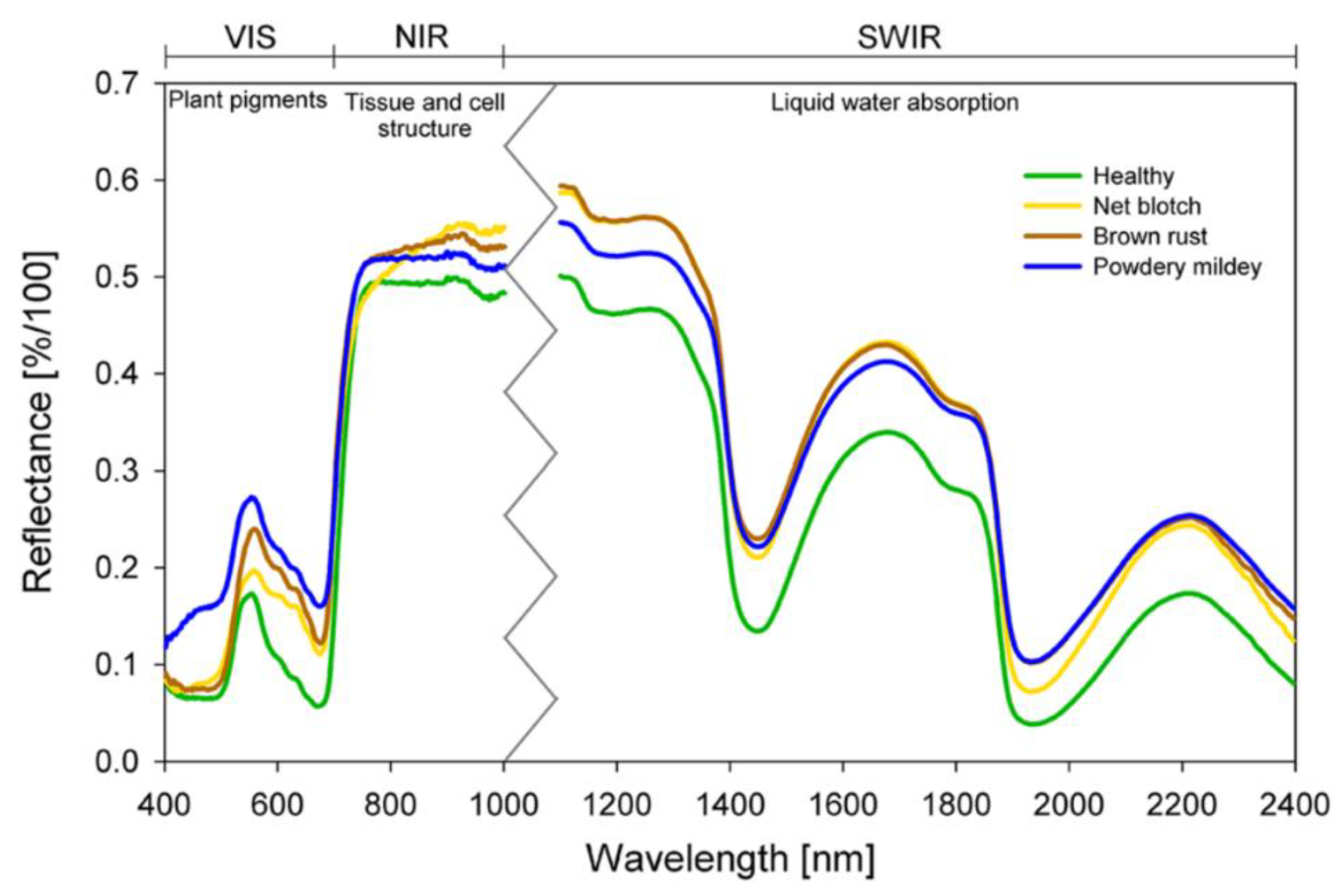
Different substances presented different reflectance and absorption values of light in specific wavebands, showing unique spectral characteristics. For example, the spectral characteristic curves of green plants are similar. They showed typical reflective spectral characteristics in some bands, which are shown in Figure 4, including the following aspects:
(1) There is a small reflection peak near 550 nm, which corresponds to the strong reflection region of chlorophyll [40];
(2) The reflectance near 700 nm increases sharply, as chlorophyll absorption had low red reflectance and high internal leaf scattering, causing high near-infrared reflectance. The slope of the curve is closely related to the content of chlorophyll in vivo in plants. This is also known as the red edge phenomenon [41];
(3) In the band between 700 and 1200 nm, strong reflectance takes place, as the leaves almost no longer absorb light energy to avoid high-temperature burns [36];
(4) There are two moisture absorption bands with low reflectance near 1470 nm and 1940 nm, which created two troughs [42];
(5) In the spectrum range of 1300~2500 nm, the spectral reflectance characteristics are mainly related to the plant moisture content and CO2 emissions [43].
Plant pathogenesis is a dynamic process in which a series of reactions occur continuously. In the process of plant–pathogen interactions, many physiological and biochemical reactions take place in vivo in plants. Based on the nutritional structure and ontogeny of different fungal pathogens, these changes in the plant pathogenesis in turn affect the optical properties of plants [44]. This makes it possible to detect plant diseases using the hyperspectral method and distinguish different diseases at each plant pathogenesis stage.
Conventionally, plant diseases are identified upon either symptoms (e.g., damage, wilt, gall, tumor, canker, wilt, rot, or necrotic disease) or visible pathogenic microorganisms (e.g., the spores in the genus rust, the mycelium or conidium in the genus erysipelas) [45]. Early plant–pathogen interactions are detected at a submillimeter size, which limits precise observation with visual assessment or HSI systems. The spatial resolution of a hyperspectral camera can be improved by using a hyperspectral microscope [46,47]. Using this approach, it is possible to study the microscopic and subtle resistance-related reactions and pathogenesis mechanisms in plants. Obtaining the hyperspectral imaging properties of the biological processes during plant–pathogen interactions enables the detection of plant diseases using hyperspectral imaging technology.
Complex processes control the emergence and progression of disease in each individual plant–pathogen system. Changes in the reflectance caused by plant disease could be attributed to the damage of specific chemical components of the leaf surfaces or tissues during pathogenesis, which could be chlorosis, the succession of necrotic tissue, or the appearance of typical fungal structures. Each host–pathogen interaction has specific and dynamic statuses in both spatial and temporal dimensions, which affects the spectral properties in different wavelength ranges [48,49,50,51].
4. Analysis Hyperspectral Imaging Information for Plant Disease Identification
Hyperspectral sensing is a non-contact and nondestructive detection method. Hyperspectral images contain a large amount of information that reveals environmental and chemical compound characteristics [51,52,53]. The challenge of hyperspectral data analysis is to extract target-related information from the huge amount of hyperspectral image data [51]. The useful information correlated with plant disease could vary during plant pathogenesis and be distributed among several regions of the measured spectrum. In recent years, a variety of data analysis methods have been applied to hyperspectral images for plant disease detection. This section reviews the most common preprocessing and analysis approaches to hyperspectral data.
4.1. Preprocessing of Hyperspectral Images
4.1.1. Image Mosaic
After the collection of crop images, it is necessary to splice several small-range images taken to obtain a complete and valuable large crop image. The mosaic of complete images is accomplished by matching pixels of the same name between images.
Fu et al. [54] reported an end-to-end deep learning method to reconstruct hyperspectral images directly from a raw mosaic image. It saves the separate demosaicing process required by other methods, which reconstruct the full-resolution RGB data from the raw mosaic image. The method reduced the computational complexity and accumulative error. Three different networks were designed based on the state-of-the-art models, including a residual network, a multiscale network, and a parallel-multiscale network. Liu et al. [55] used remote sensing images to extract the plant number information of maize seedling stages. To improve the accuracy of image mosaics, geometric reference boards were set up in different navigation belts as GPS control points to ensure subsequent mosaic work based on geographical positioning. Then the images with GPS positioning were input into Agisoft PhotoScan (Agisoft LLC, St. Petersburg, Russia) to complete the stitching process automatically. Another software, Pix4Dmapper (Pix4D S.A., Prilly, Switzerland) [56], can also automatically complete image stitching and generate high-precision normal projection images. For example, Dai et al. [57] provided a classification method of the main crops in Northern Xinjiang and He et al. [58] performed the biomass measurement of single tree trunks of Abies Minjiang using Pix4Dmapper (Pix4D S.A., Prilly, Switzerland).
4.1.2. Image Segmentation
Efficient image segmentation is important to separate the object from the background. Common image segmentation methods can be divided into three categories: region-based segmentation methods, threshold-based segmentation methods, and edge-based segmentation methods.
The selection of threshold determines the effect of image segmentation. The gray scale of the image can clearly show some characteristics of the object, so the gray histogram can be used to select the threshold of image segmentation.
Nalepa et al. [59] showed a method to effectively deal with a limited number and size of available hyperspectral ground-truth sets and apply transfer learning for building deep feature extractors. They also exploited spectral dimensionality reduction to make the technique applicable over hyperspectral data acquired using different sensors, which may capture different numbers of hyperspectral bands. The experiments were performed on several benchmarks and backed up with statistical tests. This indicates that the approach allowed for effectively training well-generalizing deep convolutional neural networks even using significantly reduced data. Cui et al. [60] proposed a novel spectral–spatial hyperspectral image classification method that exploited the spatial autocorrelation of hyperspectral images by which image segmentation was performed on the hyperspectral image to assign each pixel to a homogeneous region. Although good results were achieved, it still did not achieve the best segmentation for large field images with a complicated background, large scope, and many transformations. Therefore, it is still an urgent demand to explore innovative and efficient segmentation methods.
4.2. Vegetation Index
According to the spectral characteristics of green plants, visible and near-infrared bands can be combined to form various vegetation indices (VIS). The vegetation index method is derived from the analysis of satellite multispectral data [61]. It is also a very important tool in the process of hyperspectral data processing of medium- and near-range plant diseases. It can simply select several bands from hundreds of bands of spectral data to represent the changes in target diseases, which greatly reduces the processing cost of hyperspectral data analysis.
More than 40 VIS have been defined so far and are widely used in global and regional land cover [62,63], vegetation classification and environmental change [64,65], crop and pasture yield estimation [66,67], drought monitoring [63,68], and host–pathogen studies. Francesco et al. [69] investigated the relationships among tiger-stripe foliar symptom expression, microelements, and vegetation indices, including the NDVI, GNDVI, and WI of grapevine. The results showed that calcium could play a role in modulating the plants’ response to toxic fungal metabolites, reducing the effects of an uncontrolled reaction associated with the expression of foliar symptoms in diseased vines. Therefore, increased availability of calcium and magnesium in up to pea-sized berries reduces foliar symptom expression just when they begin to appear. Rumpf et al. [70] used nine spectral vegetation indices related to physiological parameters to be features of a support vector machine with a radial basis function as a kernel. The discrimination between healthy sugar beet leaves and diseased leaves resulted in classification accuracies of up to 97%. According to Cao et al. [71], the SPAD values were predicted by calculating the spectral fractal dimension index (SFDI) from a hyperspectral curve (420 to 950 nm). The correlation between the SPAD values and hyperspectral information was further analyzed to determine the sensitive bands that correspond to different disease levels.
Table 1 shows several examples of general spectral vegetation indices used to detect and measure the severity of various plant diseases. Formulas for defining new targeted vegetation indices can be developed for specific plant diseases, such as leaf beet disease [72]. Nevertheless, vegetation index methods abandon the spectral data of most bands. They do not fully take advantage of the potential of hyperspectral data.
4.3. Machine Learning
Hyperspectral image classification tries to define each pixel sample in the image with different categories. Machine learning hyperspectral image classification methods can be divided into unsupervised learning methods and supervised learning methods according to whether prior categories of the training samples need to be introduced.
Unsupervised learning refers to “blind” classification (clustering) based on the distribution rules of spectral features of hyperspectral images without prior knowledge. The K-means cluster and the dynamic clustering analysis methods (interactive self-organizing data analysis—ISODATA) are typical unsupervised learning methods [64].
Since plants and background regions in spectral images have significant differences in the near-infrared and red bands, Zhang et al. [73] removed the non-plant background using the K-means clustering algorithm before the detection of the scabs of rice sheath blight. Compared to the traditional background removal methods based on pixel threshold segmentation, the clustering-based method can mitigate the issue of irregular edges and the “salt and pepper” phenomenon. Based on the selected spectral features, Yuan et al. [74] developed an analytical framework for disease scab detection that combines the unsupervised classification ISODATA method and adaptive two-dimensional threshold determination. A comparison with the direct pixel-based classification results suggests that the proposed method is insensitive to differences in leaf background and can effectively identify diseased tea leaves (anthracnose) and analyze the degree of infection. The accuracies for both the calibration and validation samples were satisfactory, with an overall accuracy of 96% at the pixel level. Supervised learning is based on prior knowledge, namely labeled training samples, to learn the internal relationships between the hyperspectral image pixel samples and the corresponding categories, which are used for mapping between the unlabeled pixel samples and the corresponding categories, and finally to determine the category for unlabeled pixels. Although the classification method of supervised learning requires manually labeled training samples to assist the training classification model, its disadvantages lie in a high labor cost and strong human subjective factors. Compared to the unsupervised learning method, the classification accuracy of supervised learning can be improved through the repeated testing of prior training samples. Therefore, the supervised learning method is more popular than the unsupervised learning method. Table 2 shows the common supervised learning algorithms with their advantages and disadvantages.
The feature extraction is an essential step in the classification process that largely affects the final classification accuracy of the algorithm in comparison and combination of thermal, fluorescence early identification of root rot disease with hyperspectral reflectance [65]. In this paper, supervised machine learning classification methods were divided into conventional machine learning classification and deep learning classification according to whether the features could be automatically learned from the original hyperspectral data.
Classification methods based on ordinary machine learning can only fit the relationship between the samples and the corresponding categories according to the inherent features of the hyperspectral images or features designed by feature engineering. According to the features, the general machine learning classification method can be classified as a spectral characteristic-based classification method or a spatial spectrum joint feature-based classification method.
Conventional machine learning classification methods only use spectral features of hyperspectral images or spectral features extracted from original data through feature engineering as the basis for classification, without utilizing the spatial information of images. The methods include K-nearest neighbor (K-NN), maximum likelihood estimate (MLE), support vector machine (SVM), Fisher’s linear discrimination analysis (FLDA), naive Bayes (NB), decision tree, extreme learning machine (ELM), sparse representation-based classifier (SRC), etc.
Calderon et al. [75] applied the LDA and SVM classification methods to classify the Verticillium dahliae severity of olive using remote sensing at a large scale of 3000 ha. The LDA reached an overall accuracy of 59.0% and a kappa of 0.487, while the SVM obtained a higher overall accuracy of 79.2% and a similar kappa of 0.495. However, the LDA better classified trees at the initial and low severity levels, reaching accuracies of 71.4 and 75.0%, respectively, in comparison to the 14.3% and 40.6% obtained by the SVM. Based on the selected spectral bands, vegetation indices, and wavelet features from the canopy hyperspectral data of winter wheat, Huang et al. [76] established discriminate models using FLDA and SVM. The results indicated that FLDA was more suitable for differentiating stresses, with respective accuracies of 78.1% and 95.6% for powdery mildew and stripe rust. Karadag et al. [77] used an artificial neural network (ANN), naive Bayes (NB), and K-nearest neighbor (KNN) to classify the spectral features of healthy and fusarium diseased peppers. The average success rates were calculated as 100% for KNN, 88.125% for the ANN, and 82% for NB. Other relevant studies are provided in Table 3.
However, the label samples of hyperspectral data are limited, and most machine learning methods based on spectral features are affected by the Hughes phenomenon. The classification results often have many discrete isolated points, which are seriously inconsistent with the actual land cover distribution [90].
Hyperspectral images are characterized by high dimension, high spectral redundancy, and mixed pixels. In the case of limited label samples, it is difficult to obtain accurate classification results by directly using spectral features as the classification basis. Therefore, in recent years, several groups have introduced the spatial information of hyperspectral images based on spectral information and made up for the deficiency of spectral information only through the dependence among the spatial pixels [91]. Ghasimi et al. [92] proposed a method that combined the hidden Markov random field and the SVM classifier. The method used the hidden Markov random field to generate segmentation results and the classification results generated by the SVM to determine the classification results of the final algorithm through majority voting.
Although the above classification methods based on the space spectrum combination achieved good results, they all needed to design the classification features manually through feature engineering to improve the classification accuracy, which required a lot of time and energy to repeatedly verify. Unlike ordinary machine learning, which requires a manual design to extract the classification features, deep learning methods can automatically extract the optimal classification features.
4.4. Deep Learning
Compared to ordinary machine learning methods, deep learning has the characteristics of automatic learning and a strong classification ability and has achieved great performance improvement in many fields, such as image classification, target detection, natural language processing, and so on. Due to the rapid development of deep learning in many fields, some remote sensing image processing algorithms based on deep learning have been slowly proposed in recent years. Common deep learning algorithms used in hyperspectral image classification mainly include the stacked auto encoder (SAE) [93], deep belief network (DBN) [94], and convolutional neural networks (CNNs) [95].
A stack autoencoder network (SAE) is a deep neural network model composed of several sparse autoencoders. Usually, the output of the former autoencoder serves as the input of the latter, and the final classification result is output by a logistic (for binary classification) or SoftMax (for multiple classification) classifier. The SAE algorithm is widely used in hyperspectral image classification. For example, Chen et al. [96] extracted null spectrum features in hyperspectral images by forming a deep network of multi-layer stacked autoencoders. Wei et al. [97] combined stacked denoising autoencoders and superpixels through space constraints to improve the classification accuracy with a novel structure.
Deng et al. [98] used a UAV hyperspectral remote sensing tool for the HLB rapid detection of citrus. The proposed HLB detection methods (based on the multi-feature fusion of the vegetation index) and canopy spectral feature parameters constructed (based on the feature band in the SAE) had a classification accuracy of 99.33% and a loss of 0.0783 for the training set, and a classification accuracy of 99.72% and a loss of 0.0585 for the validation set. The field-testing results showed that the model could effectively detect the HLB plants and output the distribution of the disease in the canopy, thus judging the plant disease level in a large area efficiently.
DBN, like the SAE algorithm, is composed of multiple layers of constrained Boltzmann machines, and its generation process is essentially a process of unsupervised pre-training for each constrained Boltzmann machine. Compared to SAEs, DBNs are used less often in hyperspectral classification. Zhao et al. [99] proposed a new feature extraction and image classification framework based on a DBN for hyperspectral image classification. Zhong et al. [100] regularized the pre-training and fine-tuning stages through the a priori of potential factors for diversity enhancement, to improve the original DBN classification effect.
Sun et al. [30] used the spectral and imaging information from hyperspectral reflectance (400 similar to 1000 nm) to evaluate and classify three kinds of common peach disease (Botrytis cinerea, Rhizopus stolonifera, Colletotrichum acutatum). Three decayed stages (slight, moderate, and severe decayed peaches) were considered for classification by DBN and PLSDA. The results showed that the DBN model had better classification results than the classification accuracy of the PLSDA model. The DBN model based on integrated information (494 features) showed the highest classification results for the three diseases, with accuracies of 82.5%, 92.5%, and 100% for slightly decayed, moderately decayed, and severely decayed samples, respectively.
SAEs and DBNs are deep neural networks based on full connection. With the deepening of the network depth, the number of parameters in the model becomes extremely high, which is not conducive to subsequent training and requires great computational power. In addition, although the above deep network model can effectively extract deep features in hyperspectral images to a certain extent to enhance the discrimination among different categories, the model cannot make good use of the spatial information of hyperspectral images by converting the input data into one-dimensional vectors. In this regard, the academic community adopted the classification method based on a CNN to avoid the above problems and improve the learning and expression ability of the network more efficiently.
Table 4 shows the comparison between an ordinary neural network and a convolutional neural network. Most traditional hyperspectral classification methods used to classify research are based on the characteristics of the project. This requires a priori knowledge, and the traits are mostly shallow characteristics, but in actual research, it is not known exactly what kind of characteristics exist in the image that are the most adaptable to the problem at hand, and it requires a lot of time and energy to determine them. However, the hyperspectral image algorithm based on a CNN can automatically learn and acquire hidden advanced features in the image by constructing a multi-layer neural network and can thus obtain the classification results more efficiently and accurately.
Table 5 shows some relevant studies from recent years. For the detection of potato viruses, Polder et al. [101] designed a fully convolutional neural network that was adapted for hyperspectral images and trained on two experimental rows in the field. The trained network was validated on two other rows, with different potato cultivars. For three of the four row/date combinations, the precision and recall compared to conventional disease assessment exceeded 0.78 and 0.88, respectively. The classification of healthy and diseased wheat heads in a rapid and non-destructive manner for the early diagnosis of Fusarium head blight disease research is difficult. Zhang et al. [102] applied an improved two-dimensional CNN model to the pixels of a hyperspectral image to accurately discern the disease area. The results of the model show that the two-dimensional convolutional bidirectional gated recurrent unit neural network (2D-CNN-BidGRU) has an F1 score and accuracy of 0.75 and 0.743, respectively, which illustrates that the hybrid structure deep neural network is an excellent classification algorithm for the healthy and Fusarium head blight disease classifications in the field of hyperspectral imagery.
5. Summary
The application of hyperspectral imaging technology in agriculture makes full use of the advantages of hyperspectral mapping unity, which can precisely monitor crop growth and diseases. However, so far, hyperspectral cameras are still expensive, making them difficult to be widely applied in agriculture. The process of spectral acquisition is easily affected by environmental factors. It also takes a long time to acquire, analyze, and process the hyperspectral image data, which limits the application of hyperspectral imaging systems in agricultural real-time monitoring and online detection. When the pre-established model is applied to another index system, data analysis and model transformation are required. The characteristics of the sample may affect its classification results and prediction accuracy. In addition, hyperspectral imaging technologies have high redundancy in image processing. To reduce the time consumption of obtaining and processing hyperspectral data, it is often necessary to extract featured wavelengths for specific applications in different crops, which enables the multiple spectral imaging of the specific stresses or diseases and reduces the cost.
Other than pathogens, hyperspectral image information can also indicate stresses induced by abiotic environmental factors, crop growing process, and biological injury. With the combination of the latest machine learning models and hyperspectral data processing tools for plant disease detection, novel algorithms should be proposed to deal with complex natural conditions. Thus, other biotic or abiotic stress effects on plant spectrum features might be removed from plant disease identification models. As a result, this technology could be more useful for field practice. Meanwhile, plant disease identification models should effectively contribute to the decision support system to carry out real-time control strategies. Thus, the data processing speed should be improved with modern on-chip calculation systems such as FPGA. This means specific intellectual property kernels should be created for real-time plant disease identification and control strategy applications in later studies.
Author Contributions
Conceptualization, L.W., H.L., P.W., Y.Y. and C.L.; methodology, H.L., P.W. and Y.Y.; investigation, L.W., H.L. and P.W.; resources, A.W.; data curation, L.W. and H.L.; writing—original draft preparation, L.W. and H.L.; writing—review and editing, P.W., Y.Y. and C.L.; supervision, C.L. and P.W.; project administration, P.W.; funding acquisition, H.L., P.W. and A.W. All authors have read and agreed to the published version of the manuscript.
Funding
This research was funded by the National Natural Science Foundation of China, grant number 32001425; the Natural Science Foundation of Chongqing, China, grant numbers cstc2020jcyj-msxmX0414 and cstc2020jcyj-msxmX0459; the Key R&D Projects in the Artificial Intelligence Pilot Area of Chongqing, China, grant number cstc2021jscx-gksbX0067; the Open Funding of the Key Laboratory of Modern Agricultural Equipment and Technology (Jiangsu University), grant numbers MAET202105 and MAET202112; Local Financial Funds of the National Agricultural Science and Technology Center, Chengdu, grant number NASC2020KR05.
Acknowledgments
The authors would like to thank Lihong Wang and Qi Niu from Southwest University and Wei Ma from the Chinese Academy of Agricultural Sciences for their advice.
Conflicts of Interest
The authors declare no conflict of interest.
Abbreviations
| ANN | Artificial Neural Network |
| ARI | Anthocyanin Reflectance Index |
| ASSDN | Architecture Self-Search Deep Network |
| BRT | Boosted Regression Tree |
| BPNN | Back Propagation Neural Network |
| CARI | Carotenoid Reflectance Index |
| CNN | Convolutional Neural Networks |
| CWA | Continuous Wavelet Analysis |
| DBN | Deep Belief Network |
| DCNN | Dynamic Convolution Neural Network) |
| ELM | Extreme Learning Machine |
| FDA | Fisher Discriminant Analysis |
| FLDA | Fisher’s Linear Discrimination Analysis |
| FR | Features Ranking |
| GA | Genetic Algorithm |
| GLCM | Gray-level Co-occurrence Matrix |
| HFPSSD | Hyperspectral Feature Profile Scanning-based Scab Detection |
| HLB | HuangLongBing |
| ISODATA | Interactive Self-Organizing Data Analysis |
| KNN | K-Nearest Neighbor |
| LDA | Linear Discriminant Analysis |
| LR | Logistic Regression |
| LS | Least Squares |
| MLE | Maximum Likelihood Estimate |
| MSC | Multiplicative Scatter Correction |
| NB | Naive Bayes |
| NVDI | Normalized Difference Vegetation Index |
| PCA | Principal Component Analysis |
| PRI | Photochemical Reflectance Index |
| PSRI | Plant Senescence Reflectance Index |
| RBF | Radial Basis Function |
| RGB | Red, Green, Blue |
| RVI | Ratio Vegetation Index |
| SAE | Stacked Auto-Encoder |
| SDA | Stepwise Discriminant Analysis |
| SFDI | Spectral Fractal Dimension Index |
| SIPI | Structure Insensitive Pigment Index |
| SPA | Successive Projections Algorithm |
| SPAD | Soil and Plant Analyzer Development |
| SRC | Sparse Representation-based Classifier |
| SVM | Support Vector Machine |
| UAV | Unmanned Aerial Vehicle |
| VIS | Vegetation Indices |
| WI | Water Index |
References
- Savary, S.; Willocquet, L.; Pethybridge, S.J.; Esker, P.; McRoberts, N.; Nelson, A. The global burden of pathogens and pests on major food crops. Nat. Ecol. Evol. 2019, 3, 430–439. [Google Scholar] [CrossRef] [PubMed]
- Fisher, M.C.; Henk, D.A.; Briggs, C.J.; Brownstein, J.S.; Madoff, L.C.; McCraw, S.L.; Gurr, S.J. Emerging fungal threats to animal, plant and ecosystem health. Nature 2012, 484, 186–194. [Google Scholar] [CrossRef] [PubMed]
- Boyd, L.A.; Ridout, C.; O’Sullivan, D.M.; Leach, J.E.; Leung, H. Plant–pathogen interactions: Disease resistance in modern agriculture. Trends. Genet. 2013, 29, 233–240. [Google Scholar] [CrossRef]
- Peralta, A.L.; Sun, Y.; McDaniel, M.D.; Lennon, J.T. Crop rotational diversity increases disease suppressive capacity of soil microbiomes. Ecosphere 2018, 9, e02235. [Google Scholar] [CrossRef]
- Ristaino, J.B.; Anderson, P.K.; Bebber, D.P.; Brauman, K.A.; Wei, Q. The persistent threat of emerging plant disease pandemics to global food security. Proc. Natl. Acad. Sci. USA 2021, 118, e2022239118. [Google Scholar] [CrossRef]
- Dan, E.; Ho, T.; Rwahnih, M.A.; Martin, R.R.; Tzanetakis, I. High throughput sequencing for plant virus detection and discovery. Phytopathology 2019, 109, 716–725. [Google Scholar]
- Ma, Z.; Luo, Y.; Michailides, T.J. Nested pcr assays for detection of monilinia fructicola in stone fruit orchards and botryosphaeria dothidea from pistachios in california. J. Phytopathol. 2010, 151, 312–322. [Google Scholar] [CrossRef]
- Singh, V.; Sharma, N.; Singh, S. A review of imaging techniques for plant disease detection. Artif. Intell. Agric. 2020, 4, 229–242. [Google Scholar] [CrossRef]
- Zhu, W.; Chen, H.; Ciechanowska, I.; Spaner, D. Application of infrared thermal imaging for the rapid diagnosis of crop disease. IFAC-PapersOnLine 2018, 51, 424–430. [Google Scholar] [CrossRef]
- Cen, H.; Weng, H.; Yao, J.; He, M.; Lv, J.; Hua, S.; Li, H.; He, Y. Chlorophyll fluorescence imaging uncovers photosynthetic fingerprint of citrus Huanglongbing. Front. Plant Sci. 2017, 8, 1509. [Google Scholar] [CrossRef] [Green Version]
- Mahlein, A.K.; Kuska, M.T.; Behmann, J.; Polder, G.; Walter, A. Hyperspectral sensors and imaging technologies in phytopathology: State of the art. Annu. Rev. Phytopathol. 2018, 56, 535–558. [Google Scholar] [CrossRef] [PubMed]
- Zhang, J.; Huang, Y.; Pu, R.; Gonzalez-Moreno, P.; Yuan, L.; Wu, K.; Huang, W. Monitoring plant diseases and pests through remote sensing technology: A review. Comput. Electron. Agric. 2019, 165, 104943. [Google Scholar] [CrossRef]
- Zaneti, R.N.; Girardi, V.; Spilki, F.R.; Mena, K.; Etchepare, R. Quantitative microbial risk assessment of Sars-CoV-2 for workers in wastewater treatment plants. Sci. Total Environ. 2020, 754, 142163. [Google Scholar] [CrossRef]
- Zhang, J.; Wang, B.; Zhang, X.; Liu, P.; Huang, W. Impact of spectral interval on wavelet features for detecting wheat yellow rust with hyperspectral data. Int. J. Agr. Biolog. Eng. 2018, 11, 138–144. [Google Scholar] [CrossRef] [Green Version]
- Zhang, J.; Yang, Y.; Feng, X.; Xu, H.; He, Y. Identification of bacterial blight resistant rice seeds using terahertz imaging and hyperspectral imaging combined with convolutional neural network. Front. Plant Sci. 2020, 11, 821. [Google Scholar] [CrossRef] [PubMed]
- Jia, L.; Wang, L.; Yang, F.; Yang, L. Spring corn leaf blight monitoring based on hyperspectral derivative index. Chin. Agric. Sci. Bull. 2019, 35, 143–150. [Google Scholar]
- Lu, J.; Zhou, M.; Gao, Y.; Jiang, H. Using hyperspectral imaging to discriminate yellow leaf curl disease in tomato leaves. Precis. Agric. 2018, 19, 379–394. [Google Scholar] [CrossRef]
- Nouri, M.; Gorretta, N.; Vaysse, P.; Giraud, M.; Germain, C.; Keresztes, B.; Roger, J.M. Near infrared hyperspectral dataset of healthy and infected apple tree leaves images for the early detection of apple scab disease. Data Brief 2018, 16, 967–971. [Google Scholar] [CrossRef]
- Sandasi, M.; Vermaak, I.; Chen, W.; Viljoen, A. Skullcap and germander: Preventing potential toxicity through the application of hyperspectral imaging and multivariate image analysis as a novel quality control method. Planta Med. 2014, 80, 1329–1339. [Google Scholar] [CrossRef] [Green Version]
- Zhu, H.; Chu, B.; Zhang, C.; Liu, F.; Jiang, L.; He, Y. Hyperspectral imaging for presymptomatic detection of tobacco disease with successive projections algorithm and machine-learning classifiers. Sci. Rep. 2017, 7, 4125. [Google Scholar] [CrossRef] [Green Version]
- Hovmller, M.S.; Walter, S.; Bayles, R.A.; Hubbard, A.; Flath, K.; Sommerfeldt, N.; Leconte, M.; Czembor, P.; Rodriguez-Algaba, J.; Thach, T. Replacement of the European wheat yellow rust population by new races from the centre of diversity in the near-himalayan region. Plant Pathol. 2016, 65, 402–411. [Google Scholar] [CrossRef] [Green Version]
- Huang, L.; Zhang, H.; Chao, R.; Huang, W.; Hu, T.; Zhao, J. Detection of scab in wheat ears using in situ hyperspectral data and support vector machine optimized by genetic algorithm. Int. J. Agr. Biol. Eng. 2020, 13, 7. [Google Scholar] [CrossRef]
- Shi, Y.; Huang, W.; Zhou, X. Evaluation of wavelet spectral features in pathological detection and discrimination of yellow rust and powdery mildew in winter wheat with hyperspectral reflectance data. J. Appl. Remote Sens. 2017, 11, 026025. [Google Scholar] [CrossRef]
- Mahlein, A.K.; Alisaac, E.; Masri, A.A.; Behmann, J.; Oerke, E.C. Comparison and combination of thermal, fluorescence, and hyperspectral imaging for monitoring fusarium head blight of wheat on spikelet scale. Sensors 2019, 19, 2281. [Google Scholar] [CrossRef] [Green Version]
- Leucker, M.; Wahabzada, M.; Kersting, K.; Peter, M.; Beyer, W.; Steiner, U.; Mahlein, A.K.; Oerke, E.C. Hyperspectral imaging reveals the effect of sugar beet quantitative trait loci on cercospora leaf spot resistance. Funct. Plant Bio. 2016, 44, 1. [Google Scholar] [CrossRef] [PubMed]
- Huang, S.; Qi, L.; Xue, K.; Wang, W.; Zhu, X. Hyperspectral image analysis based on bosw model for rice panicle blast grading. Comput. Electron. Agric. 2015, 118, 167–178. [Google Scholar] [CrossRef]
- Shuaibu, M.; Lee, W.S.; Schueller, J.; Gader, P.; Hong, Y.; Kim, S. Unsupervised hyperspectral band selection for apple marssonina blotch detection. Comput. Electron. Agric. 2018, 12, 28. [Google Scholar] [CrossRef]
- Ruszczak, B.; Smykaa, K. The detection of alternaria solani infection on tomatoes using ensemble learning. J. Amb. Intel. Smart Environ. 2020, 12, 407–418. [Google Scholar] [CrossRef]
- Liang, K.; Huang, J.; He, R.; Wang, Q.; Chai, Y.; Shen, M. Comparison of Vis-NIR and SWIR hyperspectral imaging for the non-destructive detection of DON levels in Fusarium head blight wheat kernels and wheat flour. Infrared Phys. Techn. 2020, 106, 103281. [Google Scholar] [CrossRef]
- Sun, Y.; Wang, K.; Liu, Q.; Pan, L.; Tu, K. Classification and discrimination of different fungal diseases of three infection levels on peaches using hyperspectral reflectance imaging analysis. Sensors 2018, 18, 1295. [Google Scholar] [CrossRef] [Green Version]
- Wang, C.; Liu, B.; Liu, L.; Zhu, Y.; Li, X. A review of deep learning used in the hyperspectral image analysis for agriculture. Artif. Intell. Rev. 2021, 54, 5205–5253. [Google Scholar] [CrossRef]
- Xing, H.; Feng, H.; Fu, J.; Xu, X.; Yang, G. Development and Application of Hyperspectral Remote Sensing; Springer: Berlin, Germany, 2017; Volume 546, pp. 271–282. [Google Scholar]
- Telmo, A.O.; Joná, H.; Luís, P.; José, B.; Emanuel, P.; Raul, M.; Joaquim, S. Hyperspectral imaging: A review on UAV-based sensors, data processing and applications for agriculture and forestry. Remote Sens. 2017, 9, 1110. [Google Scholar]
- Thomas, S.; Kuska, M.T.; Bohnenkamp, D.; Brugger, A.; Alisaac, E.; Wahabzada, M.; Behmann, J.; Mahlein, A.K. Benefits of hyperspectral imaging for plant disease detection and plant protection: A technical perspective. J. Plant. Dis. Protect. 2018, 125, 5–20. [Google Scholar] [CrossRef]
- Gates, D.M.; Keegan, H.J.; Schleter, J.C. Sensorik für einen präzisierten Pflanzenschutz. Gesunde Pflanz. 2008, 60, 131–141. [Google Scholar]
- Wang, L.; Jia, M.; Yin, D.; Tian, J. A review of remote sensing for mangrove forests: 1956–2018. Remote Sens. Environ. 2019, 231, 111223. [Google Scholar] [CrossRef]
- Hennessy, A.; Clarke, K.; Lewis, M. Hyperspectral classification of plants: A review of waveband selection generalisability. Remote Sens. 2020, 12, 113. [Google Scholar] [CrossRef] [Green Version]
- Olli, N.; Eija, H.; Sakari, T.; Niko, V.; Teemu, H.; Xiaowei, Y.; Juha, H.; Heikki, S.; Ilkka, P.L.N.; Nilton, I. Individual tree detection and classification with UAV-based photogrammetric point clouds and hyperspectral imaging. Remote Sens. 2017, 9, 185. [Google Scholar]
- René, H.; Norbert, J.; André, G.; Jens, O. The effect of epidermal structures on leaf spectral signatures of ice plants (Aizoaceae). Remote Sens. 2015, 7, 16901. [Google Scholar]
- Liu, Y.; Zhang, G.W.; Liu, D. Simultaneous measurement of chlorophyll and water content in navel orange leaves based on hyperspectral imaging. Spectroscopy 2014, 29, 40, 42–46. [Google Scholar]
- Mutanga, O.; Van Aardt, J.; Kumar, L. Imaging spectroscopy (hyperspectral remote sensing) in Southern Africa: An overview. S. Afr. J. Sci. 2010, 105, 193–198. [Google Scholar] [CrossRef]
- Wei, A.A.; Tian, L.; Chen, X.; Yu, Y. Retrieval and application of chlorophyll-a concentration in the Poyang Lake based on exhaustion method: A case study of Chinese Gaofen-5Satellitc AHSI data. J. Huazhong Normal Univ. 2020, 54, 447–453. [Google Scholar]
- Qu, J.; Sun, D.; Cheng, J.; Pu, H. Mapping moisture contents in grass carp (ctenopharyngodon idella) slices under different freeze drying periods by vis-nir hyperspectral imaging. LWT-Food Sci. Technol. 2017, 75, 529–536. [Google Scholar] [CrossRef]
- Oerke, E. Remote sensing of diseases. Annu. Rev. Phytopathol. 2020, 58, 225–252. [Google Scholar] [CrossRef] [PubMed]
- Bonants, P.; Schoen, C.; Wolf, J.; Zijlstra, C. Developments in detection of plant pathogens and other plant-related organisms: Detection in the past towards detection in the future. Mededelingen 2001, 66, 25–37. [Google Scholar] [PubMed]
- Pu, H.; Lin, L.; Sun, D. Principles of hyperspectral microscope imaging techniques and their applications in food quality and safety detection: A review. Compr. Rev. Food Sci. F. 2019, 18, 853–866. [Google Scholar] [CrossRef] [Green Version]
- Gary, A.; Roth, S.; Tahiliani, N.M.; Neu-Baker, S.A. Hyperspectral microscopy as an analytical tool for nanomaterials. Wires. Nanomed. Nanobi. 2015, 7, 565–579. [Google Scholar]
- Mahlein, A.K.; Rumpf, T.; Welke, P.; Dehne, H.W.; Plümer, L.; Steiner, U.; Oerke, E.C. Development of spectral indices for detecting and identifying plant diseases. Remote Sens. Environ. 2013, 128, 21–30. [Google Scholar] [CrossRef]
- Mahlein, A.K.; Steiner, U.; Hillnhütter, C.; Dehne, H.W.; Oerke, E.C. Hyperspectral imaging for small-scale analysis of symptoms caused by different sugar beet diseases. Plant Methods 2012, 8, 3. [Google Scholar] [CrossRef] [Green Version]
- Wahabzada, M.; Mahlein, A.K.; Bauckhage, C.; Steiner, U.; Oerke, E.C.; Kersting, K. Plant Phenotyping using Probabilistic Topic Models: Uncovering the Hyperspectral Language of Plants. Sci. Rep. 2016, 6, 22482. [Google Scholar] [CrossRef] [Green Version]
- Behmann, J.; Mahlein, A.K.; Rumpf, T.; Romer, C.; Plumer, L. A review of advanced machine learning methods for the detection of biotic stress in precision crop protection. Precis. Agric. 2015, 16, 239–260. [Google Scholar] [CrossRef]
- Lowe, A.; Harrison, N.; French, A.P. Hyperspectral image analysis techniques for the detection and classification of the early onset of plant disease and stress. Plant Methods 2017, 13, 80. [Google Scholar] [CrossRef] [PubMed]
- Mahlein, A.K. Plant Disease Detection by Imaging Sensors-Parallels and Specific Demands for Precision Agriculture and Plant Phenotyping. Plant Dis. 2016, 100, 241–251. [Google Scholar] [CrossRef] [PubMed] [Green Version]
- Fu, H.; Bian, L.; Cao, X.; Zhang, J. Hyperspectral imaging from a raw mosaic image with end-to-end learning. Opt. Express 2020, 28, 314–324. [Google Scholar] [CrossRef]
- Liu, S.; Yang, G.; Zhou, H.; Jing, H.; Feng, H.; Xu, B.; Yang, H. Extraction of maize seedling number information based on UAV imagery. Trans. CSAE 2018, 34, 9. [Google Scholar]
- Zhang, J.; Yang, C.; Zhao, B.; Song, H.; Hoffmann, W.C.; Shi, Y.; Zhang, D.; Zhang, G. Crop Classification and LAI Estimation Using Original and Resolution-Reduced Images from Two Consumer-Grade Cameras. Remote Sens. 2017, 9, 1054. [Google Scholar] [CrossRef] [Green Version]
- Dai, J.; Zhang, G.; Guo, P.; Zeng, Y.; Cui, M.; Xue, J. Classification method of main crops in northern Xinjiang based on UAV visible waveband images. Trans. CSAE 2018, 34, 8. [Google Scholar]
- He, Y.; Zhang, Y.; Li, J.; Wang, J. Estimation of stem biomass of individual Abies faxoniana through unmanned aerial vehicle remote sensing. J. Beijing For. Univ. 2016, 38, 8. [Google Scholar]
- Nalepa, J.; Myller, M.; Kawulok, M. Transfer learning for segmenting dimensionally-reduced hyperspectral images. IEEE Geosci. Remote Sens. 2019, 17, 1228–1232. [Google Scholar] [CrossRef] [Green Version]
- Cui, B.; Ma, X.; Xie, X.; Ren, G.; Ma, Y. Classification of visible and infrared hyperspectral images based on image segmentation and edge-preserving filtering. Infrared Phys. Techn. 2017, 81, 79–88. [Google Scholar] [CrossRef]
- Ishiyama, T.; Tanaka, S.; Uchida, K.; Fujikawa, S.; Yamashita, Y.; Kato, M. Relationship among vegetation variables and vegetation features of arid lands derived from satellite data. Adv. Space Res. 2001, 28, 183–188. [Google Scholar] [CrossRef]
- Vicente-Serrano, S.M. Evaluating the impact of drought using remote sensing in a mediterranean, semi-arid region. Nat. Hazards 2007, 40, 173–208. [Google Scholar] [CrossRef]
- Zhao, X.; Zhou, D.; Fang, J. Satellite-based studies on large-scale vegetation changes in China. J. Integr. Plant Bio. 2012, 54, 713–728. [Google Scholar] [CrossRef] [PubMed]
- Zhao, J. Research on Hyperspectral Remote Sensing Images Classification Based on K-means Clustering. Geospat. Inform. 2016, 14, 4. [Google Scholar]
- Zhang, H.; Li, Y.; Jiang, H. Research status and Prospect of deep learning in hyperspectral image classification. Acta Autom. Sin. 2018, 44, 17. [Google Scholar]
- Szulczewski, W.; Zyromski, A.; Jakubowski, W.; Biniak-Pierog, M. A new method for the estimation of biomass yield of giant miscanthus (Miscanthus giganteus) in the course of vegetation. Renew. Sust. Energ. Rev. 2018, 82, 1787–1795. [Google Scholar] [CrossRef]
- Barriguinha, A.; Neto, M.D.; Gil, A. Vineyard yield estimation, prediction, and forecasting: A systematic literature review. Agronomy 2021, 11, 1789. [Google Scholar] [CrossRef]
- Zou, L.; Cao, S.; Sanchez-Azofeifa, A. Evaluating the utility of various drought indices to monitor meteorological drought in tropical dry forests. Int. J. Biometeorol. 2020, 64, 701–711. [Google Scholar] [CrossRef]
- Calzarano, F.; Pagnani, G.; Pisante, M.; Bellocci, M.; Cillo, G.; Metruccio, E.G.; Di Marco, S. Factors involved on tiger-stripe foliar symptom expression of esca of grapevine. Plants 2021, 10, 1041. [Google Scholar] [CrossRef]
- Rumpf, T.; Mahlein, A.K.; Steiner, U.; Oerke, E.C.; De Hne, H.W.; Plümer, L. Early detection and classification of plant diseases with support vector machines based on hyperspectral reflectance. Comput. Electron. Agr. 2010, 74, 91–99. [Google Scholar] [CrossRef]
- Cao, Y.F.; Xu, H.L.; Song, J.; Yang, Y.; Hu, X.H.; Wiyao, K.T.; Zhai, Z.Y. Applying spectral fractal dimension index to predict the spad value of rice leaves under bacterial blight disease stress. Plant Methods 2022, 18, 67. [Google Scholar] [CrossRef]
- Sims, D.A.; Gamon, J.A. Relationships between leaf pigment content and spectral reflectance across a wide range of species, leaf structures and developmental stages. Remote Sens. Environ. 2002, 81, 337–354. [Google Scholar] [CrossRef]
- Zhang, J.C.; Tian, Y.Y.; Yan, L.J.; Wang, B.; Wang, L.; Xu, J.F.; Wu, K.H. Diagnosing the symptoms of sheath blight disease on rice stalk with an in-situ hyperspectral imaging technique. Biosyst. Eng. 2021, 209, 94–105. [Google Scholar] [CrossRef]
- Yuan, L.; Yan, P.; Han, W.; Huang, Y.; Bao, Z. Detection of anthracnose in tea plants based on hyperspectral imaging. Comput. Electron. Agr. 2019, 167, 105039. [Google Scholar] [CrossRef]
- Calderon, R.; Navas-Cortes, J.A.; Zarco-Tejada, P.J. Early detection and quantification of verticillium wilt in olive using hyperspectral and thermal imagery over large areas. Remote Sens. 2015, 7, 5584–5610. [Google Scholar] [CrossRef] [Green Version]
- Huang, W.; Lu, J.; Ye, H.; Kong, W.; Yue, S. Quantitative identification of crop disease and nitrogen-water stress in winter wheat using continuous wavelet analysis. Int. J. Agr. Biol. Eng. 2018, 11, 8. [Google Scholar] [CrossRef] [Green Version]
- Karadag, K.; Tenekeci, M.E.; Tasaltin, R.; Bilgili, A. Detection of pepper fusarium disease using machine learning algorithms based on spectral reflectance. Sustain. Comput Inform. Syst. 2020, 28, 100299. [Google Scholar] [CrossRef]
- Xie, C.; Yang, C.; He, Y. Hyperspectral imaging for classification of healthy and gray mold diseased tomato leaves with different infection severities. Comput. Electron. Agr. 2017, 135, 154–162. [Google Scholar] [CrossRef]
- Lu, J.; Ehsani, R.; Shi, Y.; Abdulridha, J.; Castro, A.D.; Xu, Y. Field detection of anthracnose crown rot in strawberry using spectroscopy technology. Comput. Electron. Agric. 2017, 135, 289–299. [Google Scholar] [CrossRef]
- Weng, H.Y.; Lv, J.W.; Cen, H.Y.; He, M.B.; Zeng, Y.B.; Hua, S.J.; Li, H.Y.; Meng, Y.Q.; Fang, H.; He, Y. Hyperspectral reflectance imaging combined with carbohydrate metabolism analysis for diagnosis of citrus Huanglongbing in different seasons and cultivars. Sens. Actuators B-Chem. 2018, 275, 50–60. [Google Scholar] [CrossRef]
- Nagasubramanian, K.; Jones, S.; Sarkar, S.; Singh, A.K.; Singh, A.; Ganapathysubramanian, B. Hyperspectral band selection using genetic algorithm and support vector machines for early identification of charcoal rot disease in soybean stems. Plant Methods 2018, 14, 86. [Google Scholar] [CrossRef]
- Abdulridha, J.; Batuman, O.; Ampatzidis, Y. Uav-based remote sensing technique to detect citrus canker disease utilizing hyperspectral imaging and machine learning. Remote Sens. 2019, 11, 1373. [Google Scholar] [CrossRef] [Green Version]
- Deng, X.; Huang, Z.; Zheng, Z.; Lan, Y.; Dai, F. Field detection and classification of citrus huanglongbing based on hyperspectral reflectance. Comput. Electron. Agr. 2019, 167, 105006. [Google Scholar] [CrossRef]
- Lin, F.; Guo, S.; Tan, C.; Zhou, X.; Zhang, D. Identification of rice sheath blight through spectral responses using hyperspectral images. Sensors 2020, 20, 6243. [Google Scholar] [CrossRef] [PubMed]
- Vijver, R.; Mertens, K.; Heungens, K.; Somers, B.; Saeys, W. In-field detection of Alternaria solani in potato crops using hyperspectral imaging. Comput. Electron. Agr. 2019, 168, 105106. [Google Scholar] [CrossRef]
- Zhang, D.; Chen, G.; Zhang, H.; Jin, N.; Chen, Y. Integration of spectroscopy and image for identifying fusarium damage in wheat kernels using hyperspectral imaging. Spectrochim. Acta A 2020, 236, 118344. [Google Scholar] [CrossRef] [PubMed]
- Gu, Q.; Sheng, L.; Zhang, T.H.; Lu, Y.W.; Zhang, Z.J.; Zheng, K.F.; Hu, H.; Zhou, H.K. Early detection of tomato spotted wilt virus infection in tobacco using the hyperspectral imaging technique and machine learning algorithms. Comput. Electron. Agr. 2019, 167, 105066. [Google Scholar] [CrossRef]
- Calamita, F.; Imran, H.A.; Vescovo, L.; Mekhalfi, M.L.; Porta, N.L. Early identification of root rot disease by using hyperspectral reflectance: The case of pathosystem grapevine/armillaria. Remote Sens. 2021, 13, 2436. [Google Scholar] [CrossRef]
- Zhao, X.H.; Zhang, J.C.; Huang, Y.B.; Tian, Y.Y.; Yuan, L. Detection and discrimination of disease and insect stress of tea plants using hyperspectral imaging combined with wavelet analysis. Comput. Electron. Agr. 2022, 193, 106717. [Google Scholar] [CrossRef]
- Du, P.; Xia, J.; Xue, Z.; Tan, K.; Su, H.; Bao, R. Research progress of hyperspectral remote sensing image classification. Remote Sens. Bull. 2016, 20, 21. [Google Scholar]
- Hou, P.; Yao, M.; Jia, W.; Zhang, F.; Wang, D. Spatial spectrum discriminant analysis for hyperspectral image classification. Opt. Precis. Eng. 2018, 26, 450–460. [Google Scholar]
- Ghasimi, P.; Benediktsson, J.A.; Ulfarsson, M.O. The spectral-spatial classification of hyperspectral images based on Hidden Markov Random Field. IEEE T. Geosci. Remote Sens. 2014, 52, 2565–2574. [Google Scholar]
- Hinton, G.E.; Salakhutdinov, R.R. Reducing the Dimensionality of Data with Neural Networks. Science 2006, 313, 504–507. [Google Scholar] [CrossRef] [PubMed] [Green Version]
- Hinton, G.E.; Osindero, S.; Teh, Y.W. A Fast Learning Algorithm for Deep Belief Nets. Neural Comput. 2014, 18, 1527–1554. [Google Scholar] [CrossRef]
- Krizhevsky, A.; Sutskever, I.; Hinton, G.E. ImageNet Classification with Deep Convolutional Neural Networks. Commun. ACM 2012, 25, 1097–1105. [Google Scholar] [CrossRef]
- Wei, F.; Li, S.; Fang, L. Spectral-spatial hyperspectral image classification via superpixel merging and sparse representation. IEEE Geosci. Remote. Sens. 2015, 18, 861–865. [Google Scholar]
- Zhao, X.; Chen, Y.; Jia, X. Spectral-Spatial Classification of Hyperspectral Data Based on Deep Belief Network. IEEE J. Sel. Top. Appl. Earth Obs. Remote Sens. 2015, 8, 2381–2392. [Google Scholar]
- Deng, X.L.; Zhu, Z.H.; Yang, J.C.; Zheng, Z.; Huang, Z.X.; Yin, X.B.; Wei, S.J.; Lan, Y.B. Detection of citrus huanglongbing based on multi-input neural network model of uav hyperspectral remote sensing. Remote Sens. 2020, 12, 2678. [Google Scholar] [CrossRef]
- Zhong, P.; Gong, Z.; Li, S.; Schonlieb, C.B. Learning to Diversify Deep Belief Networks for Hyperspectral Image Classification. IEEE T. Geosci. Remote 2017, 55, 3516–3530. [Google Scholar] [CrossRef]
- Fazari, A.; Pellicer-Valero, O.J.; Gomez-SancHs, J.; Bernardi, B.; Blasco, J. Application of deep convolutional neural networks for the detection of anthracnose in olives using vis/nir hyperspectral images. Comput. Electron. Agr. 2021, 187, 106252. [Google Scholar] [CrossRef]
- Polder, G.; Blok, P.M.; Villiers, H.; Wolf, J.; Kamp, J. Potato virus detection in seed potatoes using deep learning on hyperspectral images. Front. Plant Sci. 2019, 10, 209. [Google Scholar] [CrossRef] [Green Version]
- Zhang, X.; Han, L.; Dong, Y.; Shi, Y.; Sobeih, T. A deep learning-based approach for automated yellow rust disease detection from high-resolution hyperspectral uav images. Remote Sens. 2019, 11, 1554. [Google Scholar] [CrossRef] [Green Version]
- Xiu, J.; Lu, J.; Shuai, W.; Hai, Q.; Shao, L. Classifying wheat hyperspectral pixels of healthy heads and fusarium head blight disease using a deep neural network in the wild field. Remote Sens. 2018, 10, 395. [Google Scholar]
- Feng, L.; Wu, B.; Zhu, S.; Wang, J.; Zhang, C. Investigation on data fusion of multisource spectral data for rice leaf diseases identification using machine learning methods. Front. Plant Sci. 2020, 11, 577063. [Google Scholar] [CrossRef] [PubMed]
- Hernandez, I.; Gutierrez, S.; Ceballos, S.; Iniguez, R.; Barrio, I.; Tardaguila, J. Artificial intelligence and novel sensing technologies for assessing downy mildew in grapevine. Horticulturae 2021, 7, 103. [Google Scholar] [CrossRef]
- Nguyen, C.; Sagan, V.; Maimaitiyiming, M.; Maimaitijiang, M.; Bhadra, S.; Kwasniewski, M.T. Early detection of plant viral disease using hyperspectral imaging and deep learning. Sensors 2021, 21, 742. [Google Scholar] [CrossRef] [PubMed]
- Lv, Y.P.; Lv, W.B.; Han, K.X.; Tao, W.T.; Zheng, L.; Weng, S.Z.; Huang, L.S. Determination of wheat kernels damaged by fusarium head blight using monochromatic images of effective wavelengths from hyperspectral imaging coupled with an architecture self-search deep network. Food Control 2022, 135, 108819. [Google Scholar]
Figure 1.
Number of published relevant literature records each year. (a) Keywords “hyperspectral” and “plants”; (b) keywords “hyperspectral”, “plants”, and “disease”.
Figure 1.
Number of published relevant literature records each year. (a) Keywords “hyperspectral” and “plants”; (b) keywords “hyperspectral”, “plants”, and “disease”.

Figure 2.
Structure of a hyperspectral image data cube of a cucumber leaf.

Figure 3.
Interaction between natural light and plant leaf surface.

Figure 4.
Spectral signatures of healthy barley leaves (green) and diseased barley leaves with net blotch (yellow), brown rust (brown), and powdery mildew (blue), respectively, at 10 days after inoculation. Sensors: “PS V10E” (400–1000 nm) and “SWIR” (1000–2500 nm) push broom scanners (Specim, Oulu, Finland). A zigzag line has been added to separate the discontinuous parts of the spectral curves. All measurements were taken with the HyperART setup according to Thomas et al. [34] (Reprinted with permission, copyright 2022 Anne-Katrin Mahlein). VIS—visual, NIR—near-infrared, SWIR—shortwave infrared (parts of the electromagnetic spectrum).


Table 1.
Application of general spectral vegetation indices.
| Vegetation Index | Formula | Application |
|---|---|---|
| Normalized difference vegetation index (NDVI) | (R800 − R670)/(R800 + R670) | Detecting vegetation coverage, related to chlorophyll content. |
| Green normalized difference vegetation index (GNDVI) | (NIR − GREEN)/(NIR + GREEN) | Detecting withered or aged crops and measuring the nitrogen content in leaves in the absence of red bands. |
| Water index (WI) | R900/R970 | Estimating the water stress. |
| Ratio vegetation index (RVI) | R800/R670 | Detecting and estimating plant biomass, related to chlorophyll content. |
| Plant senescence reflectance index (PSRI) | (R680 − R500)/R750 | Detecting plant senescence, related to pigment content. |
| Carotenoid reflectance index (CARI) | 1/R510 − 1/R550 | Related to carotenoid content. |
| Anthocyanin reflectance index (ARI) | 1/R510 − 1/R700 | Detecting yellow rust of wheat, related to anthocyanin content. |
| Photochemical reflectance index (PRI) | (R570 − R531)/(R570 + R531) | Detecting yellow rust of wheat, related to photosynthesis and carotenoid content. |
| Structure insensitive pigment index (SIPI) | (R800 − R445)/R800 + R680) | Related to the ratio of carotinoids and chlorophylla. |
Table 2.
Comparison of supervised learning algorithms.
| Method | Advantage | Disadvantage |
|---|---|---|
| K-NN | (1) The theory has matured and easy application. (2) Less training time. | (1) High computational complexity and spatial complexity. (2) Sample imbalance. |
| NBM | (1) Performs well for small-scale data and is suitable for multi-classification. (2) Simple computation. | (1) Due to the emphasis on conditional independence, the accuracy is reduced. (2) Sensitive to the expression of input data. |
| A priori probability needs to be calculated. | ||
| MLE | It can quickly specify the pixels to be classified into one of several classes. | When there are many types of hyperspectral data, the operation speed slows down significantly, and more training samples are needed. |
| Decision Tree | (1) Low computing cost. (2) Able to handle irrelevant features. (3) Suitable for datasets with many attributes and has high scalability. | (1) Easy to cause over-fitting. (2) When all kinds of samples are unbalanced, the result of information gain will be biased to the characteristics with more data values. |
| ELM | Has fast learning speed and good generalization ability. | The parameters of the model are randomly selected, which causes ELM instability. |
| SRC | Low computing cost. | Various sub-dictionaries have high atomic correlation, and similar samples may be linearly represented by different sub-dictionaries, resulting in poor classification accuracy. |
| SVM | (1) Low generalization error rate, low computing cost. (2) It can solve the classification problem of small-sample and high-dimensional data. | It is sensitive to parameter adjustment and function selection. |
| Has good classification effect. |
Table 3.
Recent advances in plant disease detection based on machine learning.
| Reference | Pathosystem | Scale | Methods | Detection | Early Detection | Precision |
|---|---|---|---|---|---|---|
| Calderon et al. (2015) [75] | Olive—Verticillium wilt | Canopy | LDA, SVM | ✓ | Overall: LDA 59.0%, SVM 79.2% Early detection: LDA 75.0%, SVM 40.6%. | |
| Xie et al. (2017) [78] | Tomato—Gray mold disease | Leaf | KNN, C5.0, FR-KNN | ✓ | Detection: 94.44%, 94.44%, 97.22% (KNN, C5.0, KNN) Early detection: 66.67%, 66.67%, 41.67% | |
| Lu et al. (2017) [79] | Strawberry—Anthracnose crown rot | Leaf | SDA, FDA, KNN | ✓ | ✓ | SDA: 71.3%, FDA: 70.05%, KNN: 73.6% |
| Zhu et al. (2017) [20] | Tobacco—Mosaic virus | Leaf | SPA–GLCM–BPNN/ELM/ SVM | ✓ | 95.00% | |
| Huang et al. (2018) [76] | Wheat—Powdery mildew, stripe rust | Canopy | FLDA, SVM | ✓ | FLDA: Powdery mildew 78.1%, stripe rust 95.6% | |
| Weng et al. (2018) [80] | Citrus—Huanglongbing, Fe deficient | Leaf | LS–SVM | 93.50% | ||
| Nagasubramanian et al. (2018) [81] | Sugar beet—Cercospora leaf spot | stem | GA–SVM | ✓ | Detection: 97% Early detection: 90.91% | |
| Abdulridha et al. (2019) [82] | Citrus—Canker | Leaf/canopy | RBF, KNN | ✓ | Leaf: 94%, 95%, 96% (asymptomatic, early, and late symptoms) Canopy: 94%, 96%, 100% | |
| Mahlein et al. (2019) [24] | Wheat—Fusarium head blight | Spikelet | SVM | ✓ | Detection: 89.0% Early detection: 78.0% | |
| Deng et al. (2019) [83] | Citrus—Huanglongbing | Leaf | SVM | ✓ | ✓ | Detection: 96% Early Detection: 90.8% |
| Lin et al. (2020) [84] | Rice—Sheath blight | Leaf | Relief decision tree | 95.50% | ||
| Van de Vijver et al. (2020) [85] | Potato—Early blight | Leaf | PLS–DA, PCA–SVM, decision tree | ✓ | 92.78% | |
| Karadag et al. (2020) [77] | Pepper—Fusarium disease, mycorrhizal fungus | Leaf | KNN, ANN, NB | KNN: 100%, ANN: 88.125%, NB: 82% | ||
| Zhang et al. (2020) [86] | Wheat—Fusarium head blight | Leaf | SPA-RF | 96.44% | ||
| Gu et al. (2020) [87] | Tobacco—Tomato spotted wilt virus | Leaf | SPA–BRT | ✓ | 85.20% | |
| Yuan et al. (2020) [74] | Tea—Anthracnose | Leaf | ISODATA | Pixel level: 98% Patch level: 94% | ||
| Calamita et al. (2021) [88] | Vitis vinifera—Fungi infection | Leaf | NB | ✓ | Detection: 90% Early detection: 75% | |
| Zhang et al. (2021) [73] | Rice—Sheath blight | Leaf | K-means–FLDA–HFPSSD | Pixel level: 98.42% Patch level: 95.92% | ||
| Zhao et al. (2022) [89] | Tea—Green leafhopper, anthracnose, sunburn | Leaf | CWA–K-means, SVM–RF | Green leafhopper: 93.99–94.20%, Anthracnose 94.12–94.28%, Sunburn 82.50–83.91% |
Table 4.
Comparison of ANN and CNN.
| Method | Advantages | Disadvantages |
|---|---|---|
| ANN | Able to learn advanced features of data automatically and has excellent classification performance. | (1) The model requires huge parameters and high computational force. (2) The input is a one-dimensional vector, which cannot make good use of map spatial information. (3) Difficult training, easy to produce gradient disappearance. |
| CNN | (1) Able to learn advanced features of data automatically and has excellent classification performance. (2) Compared to the ANN, the CNN model requires significantly fewer data parameters and trains faster. | The existence of a pooling layer may lead to the loss of valuable information while ignoring the relationship between the global and local scales. |
Table 5.
Recent advances in plant disease detection based on deep learning.
| Reference | Host–Pathogen System | Scale | Methods | Field Capable | Early Detection | Precision |
|---|---|---|---|---|---|---|
| Sun et al. (2018) [30] | Peach—Botrytis cinerea, Rhizopus stolonifera, Colletotrichum acutatum | Flesh | PCA–DBN | ✓ | Detection: 92.5% Early Detection: 82.5% | |
| Jin et al. (2018) [103] | Wheat—Fusarium head blight | Kernels | CNN | ✓ | 74.30% | |
| Polder et al. (2019) [101] | Potato—Viruses | Leaf | CNN | ✓ | ✓ | 78.00% |
| Zhang et al. (2019) [102] | Wheat—Yellow rust | canopy | DCNN | ✓ | 85% | |
| Deng et al. (2020) [98] | Citrus—Huanglongbing | canopy | SAE | ✓ | 99.72% | |
| Liang et al. (2020) [29] | Wheat—Fusarium head blight | Kernels/Flour | MSC–GA–SAE | Kernels: 100% Flour: 96% | ||
| Zhang et al. (2020) [15] | Rice—Bacterial blight | Leaf | CNN | 82.60% | ||
| Feng et al. (2020) [104] | Rice—Leaf blight, rice blast, rice sheath blight | Leaf | SVM, LR, CNN | 93.00% | ||
| Fazari et al. (2021) [100] | Olive—Anthracnose | Leaf | CNN | ✓ | Detection: 100% Early Detection: 85% | |
| Hernandez et al. (2021) [105] | Grape—Downy mildew | Leaf | KNN, CNN | ✓ | CNN: 82% KNN: 66% | |
| Nguyen et al. (2021) [106] | Grape—Grapevine vein-clearing virus | vine | 2D CNN, 3D CNN | ✓ | 2D CNN:71% 3D CNN: 75% | |
| Liu et al. (2022) [107] | Wheat—Fusarium head blight | kernels | ASSDN | 98.31% |
Publisher’s Note: MDPI stays neutral with regard to jurisdictional claims in published maps and institutional affiliations. |
© 2022 by the authors. Licensee MDPI, Basel, Switzerland. This article is an open access article distributed under the terms and conditions of the Creative Commons Attribution (CC BY) license (https://creativecommons.org/licenses/by/4.0/).
Share and Cite
MDPI and ACS Style
Wan, L.; Li, H.; Li, C.; Wang, A.; Yang, Y.; Wang, P. Hyperspectral Sensing of Plant Diseases: Principle and Methods. Agronomy 2022, 12, 1451. https://0-doi-org.brum.beds.ac.uk/10.3390/agronomy12061451
AMA Style
Wan L, Li H, Li C, Wang A, Yang Y, Wang P. Hyperspectral Sensing of Plant Diseases: Principle and Methods. Agronomy. 2022; 12(6):1451. https://0-doi-org.brum.beds.ac.uk/10.3390/agronomy12061451
Chicago/Turabian StyleWan, Long, Hui Li, Chengsong Li, Aichen Wang, Yuheng Yang, and Pei Wang. 2022. "Hyperspectral Sensing of Plant Diseases: Principle and Methods" Agronomy 12, no. 6: 1451. https://0-doi-org.brum.beds.ac.uk/10.3390/agronomy12061451
Note that from the first issue of 2016, this journal uses article numbers instead of page numbers. See further details here.