Biomass Prediction of Heterogeneous Temperate Grasslands Using an SfM Approach Based on UAV Imaging


Grassland Science and Renewable Plant Resources, Faculty of Organic Agricultural Science, Universität Kassel, Steinstraße 19, 37213 Witzenhausen, Germany
*
Author to whom correspondence should be addressed.
Agronomy 2019, 9(2), 54; https://0-doi-org.brum.beds.ac.uk/10.3390/agronomy9020054
Submission received: 7 November 2018
/
Revised: 15 January 2019
/
Accepted: 23 January 2019
/
Published: 26 January 2019
(This article belongs to the Special Issue Remote Sensing Application for Monitoring Grassland and Forage Production)
Abstract
:An early and precise yield estimation in intensive managed grassland is mandatory for economic management decisions. RGB (red, green, blue) cameras attached on an unmanned aerial vehicle (UAV) represent a promising non-destructive technology for the assessment of crop traits especially in large and remote areas. Photogrammetric structure from motion (SfM) processing of the UAV-based images into point clouds can be used to generate 3D spatial information about the canopy height (CH). The aim of this study was the development of prediction models for dry matter yield (DMY) in temperate grassland based on CH data generated by UAV RGB imaging over a whole growing season including four cuts. The multi-temporal study compared the remote sensing technique with two conventional methods, i.e., destructive biomass sampling and ruler height measurements in two legume-grass mixtures with red clover (Trifolium pratense L.) and lucerne (Medicago sativa L.) in combination with Italian ryegrass (Lolium multiflorum Lam.). To cover the full range of legume contribution occurring in a practical grassland, pure stands of legumes and grasses contained in each mixture were also investigated. The results showed, that yield prediction by SfM-based UAV RGB imaging provided similar accuracies across all treatments (R2 = 0.59–0.81) as the ruler height measurements (R2 = 0.58–0.78). Furthermore, results of yield prediction by UAV RGB imaging demonstrated an improved robustness when an increased CH variability occurred due to extreme weather conditions. It became apparent that morphological characteristics of clover-based canopies (R2 = 0.75) allow a better remotely sensed prediction of total annual yield than for lucerne-grass mixtures (R2 = 0.64), and that these crop-specific models cannot be easily transferred to other grassland types.
1. Introduction
Legume-grass mixtures with red clover (Trifolium pratense L.) and lucerne (Medicago sativa L.) in combination with Italian ryegrass (Lolium multiflorum Lam.), grown for 1–3 years, play an important role in crop rotations, particularly in organic farming in temperate European climates. Such crops serve as green manure by fixing nitrogen or as feedstock for animals and biogas plants. These intensive grasslands are harvested three to five times per year and, therefore, an early and precise yield estimation is mandatory for management decisions and economic optimizations at the field and farm level [1]. An emerging and promising technology in grassland faming is remote sensing, and especially the use of different sensors on unmanned aerial vehicles (UAV) show great potential for improving agricultural use of grasslands [2,3].
Destructive biomass sampling is considered to be the most accurate yield estimation method but can also be considered as the most labor-intensive method [4]. Another approach for estimating biomass in grasslands is the assessment of canopy height (CH), which was frequently found to be positively correlated with crop biomass [5,6]. Traditional height measurements in grassland are often conducted with a rising plate meter, determining the compressed sward height, or with a ruler stick [7,8]. Furthermore, several portable technical devices for non-destructive biomass estimation were developed in the recent years, which so far were not widely distributed in agricultural practice, e.g., leaf area meter to asses leaf area index (LAI) [9], electronic capacitance meter, which measures the difference of capacitance between air and biomass [1] and a reflectometer, which measures intensity of spectral reflectance by light emitting diodes (LED) [10]. Biomass sampling, manual height measurement and the above mentioned technical devices need a substantial number of repetitions in combination with a spatially uniform distributions of the measurements to generate a reliable yield estimation [11]. Therefore, much time and effort is required to receive reliable data especially on large areas.
Sensors attached on UAVs are useful non-destructive tools for obtaining spatial information from large and remote areas. There exist different sensor systems, such as LiDAR, ultrasound and RGB (red, green, blue) imaging to collect spatial data for a rapid quantification of aboveground biomass [3,12,13,14]. A UAV in combination with a consumer-grade digital camera for RGB imaging represents a low-cost approach for estimating yield, which may be affordable und workable for farmers. By photogrammetric structure from motion (SfM) processing of the UAV-based images into point clouds, 3D spatial data can be easily generated. Forsmoo et al. [14] calculated in a grassland sward, that for a plot of 8 m2 a CH assessment with a ruler needed 550 single height measurements to receive the same accuracy as a SfM-based CH assessment based on UAV RGB imaging. Therefore, the high spatial resolution makes UAV RGB imagery in combination with an SfM approach an interesting tool for yield estimation in practical grassland farming.
SfM derived height measurement based on UAV RGB imaging was successfully used in forestry [15], and, to a lower degree also in agricultural crops, such as wheat [6,16], barley [17], maize [18,19] and vegetable crops [20]. All these studies found strong relationships between biomass and RGB imaging in homogeneous crops. Contrary, grassland represents a mixed crop containing legumes and grasses of several species. Additionally, species contribution and yield changes in the field throughout the growing season and is affected by many factors, such as cutting intensity, soil features, fertilization and climate conditions [21,22]. So far, only a few studies exist using SfM based on RGB imaging in grassland. Cooper et al. [23] and Wallace et al. [13] compared height measurements in permanent grasslands based on terrestrial SfM and terrestrial LiDAR and observed similar relationships between these two methods and the grassland biomass. Van Iersel et al. [24] showed the potential of modeling temporal dynamics of CH in a floodplain grassland and of classifying different vegetation types (pixel size = 5 cm) with a consumer-grade camera attached on a UAV. Viljanen et al. [25] worked in an intensive grassland with four harvest cuts and different nitrogen applications rates. The latter used a high-resolution camera (pixel size = 1 cm) mounted on a UAV and combined CH with spectral vegetation indices (VI), resulting in highly significant correlations with biomass. VIs from multi- or hyperspectral sensors also show promising potential for qualitative and quantitative biomass estimation; however extensive spectral calibration work is necessary for these technique [3].
To understand the spatial variability and dynamics in grasslands over the entire growing season multi-temporal studies are needed. So far, no study using yield prediction models by SfM considered different proportions of legumes (including pure legume and grass stands as well as legume-grass mixtures), which frequently occur in practical grassland farming. The aim of this study is the development of estimation models for dry matter yield (DMY) in mixed grassland by CH generated by UAV RGB imaging over a whole growing season. The study compares this novel remote sensing technique with ruler height measurements, an established conventional method and uses destructive biomass sampling as a reference data. All measurements were conducted in two different legume-grass mixtures. To cover the wide range of legume contribution in practical grassland, pure stands of legumes (100% legumes) and grasses (0% legumes) were investigated as well as their mixtures. The specific objectives of this study were: (1) the assessment of CH by RGB imaging in two legumes-grass mixtures over the whole growing season; (2) the comparison of prediction models based on an SfM approach with a conventional measurement method; (3) the development of a yield prediction model containing also pure stands of legumes and grasses; (4) assessment of the prediction accuracy for the total annual DMY based on SfM including all harvest cuts during one complete growing season.
2. Materials and Methods
2.1. Experimental Site and Design
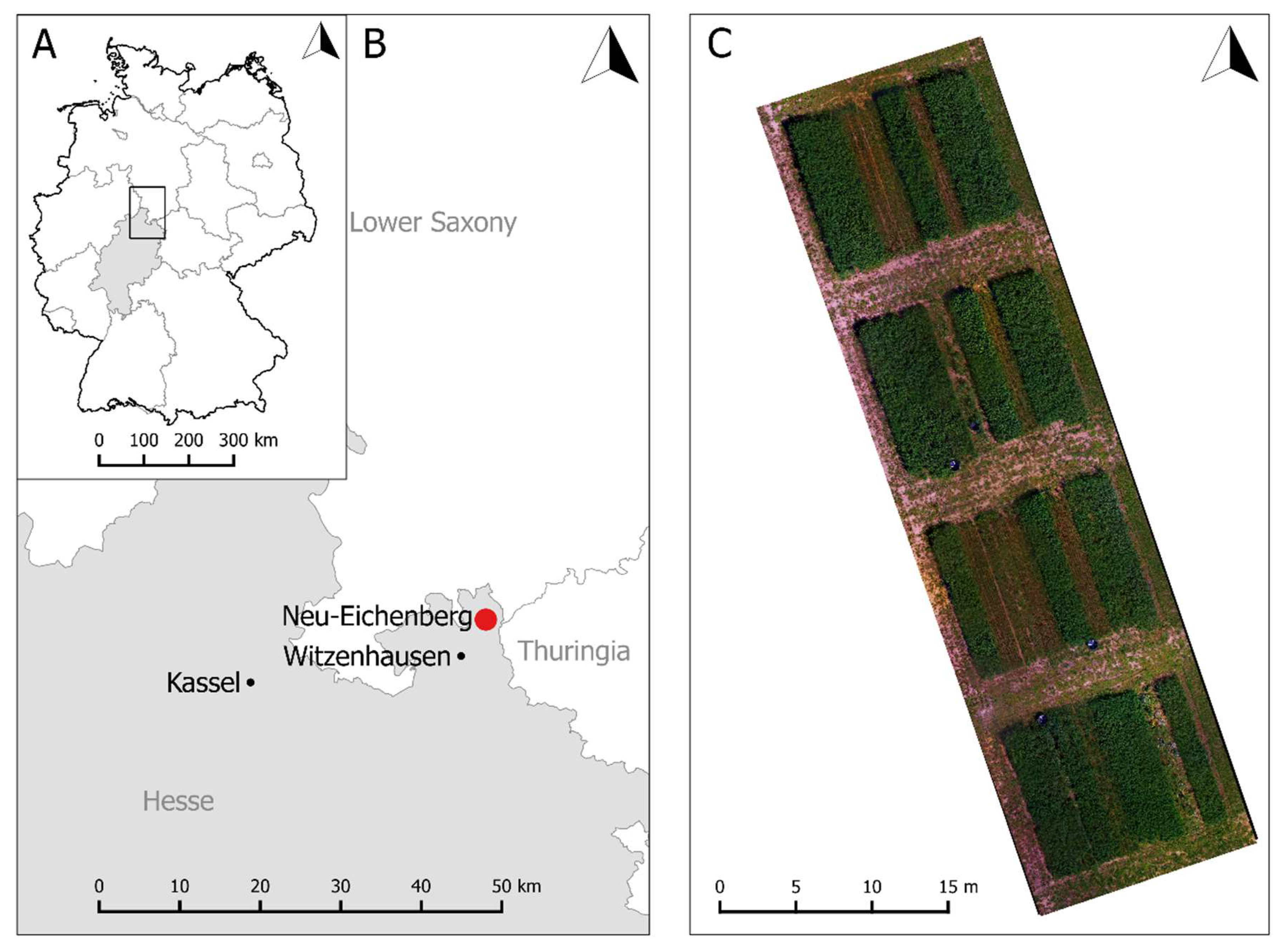
The study was carried out at the experimental farm in Neu-Eichenberg of the Universität Kassel (51°23’ N, 9°54’ E, 227 m above sea level) in northern Hesse, Germany. The soil is a silty clay loam with 3.6% sand, 73% silt, 23.4% clay and 2% humus. Summer barley was cultivated as a preceding crop. The mean annual precipitation and daily temperature of the site is 728 mm and 8 °C, respectively (Figure 1A,B).
Field plots (1.5 m × 10 m) of clover-grass (CG) and lucerne-grass (LG) in mixtures as well as of pure stands of legumes (L; 100% legumes) and grasses (G; 0% legumes) (Table 1) were sown in autumn of 2016 in four randomized replicate blocks, giving a total of 24 plots (Figure 1C). All treatments were sown with a total seed rate of 35 kg ha−1. CG contained 60% Lolium multiflorum, 30% Trifolium pratense, 5% Trifolium hybridum L. and 5% Trifolium repens L., whereas LG included 40% Medicago sativa, 20% Festuca pratensis Huds., 15% Lolium perenne L., 10% Lolium multiflorum, 10% Trifolium pratense and 5% Phleum pretense L. Consequently, the treatments formed a set of heterogenous vegetation which differed largely in their morphological and optical characteristics. As the experimental farm is managed organically, no fertilizer or pesticides were applied.
The total amount of rainfall (762 mm in 2017) was higher than the mean annual precipitation (728 mm), though early summer was characterized by a severe drought. Precipitation for the first cut (17 May 2017) revealed 66 mm compared to long-term average of 91 mm and for the second cut (26 June 2017) 47 mm compared to long-term average of 95 mm. This drought caused an accelerated maturation of the grasses with pronounced stem formation and little leaf growth especially in the second cut.
2.2. RGB Remote Sensing and Data Acquisition
RGB images were taken with a low-cost quadrocopter (DJI Phantom 3 Advanced; Shenzhen, China). The flight plan was done with autopilot by means of Pix4Dcapture software (App version 4.4.0, Pix4D SA, Lausanne, Switzerland). All missions were carried out in the morning to ensure equal sun position (8:00–12:00 a.m.). RGB images were taken one day before every harvest (4 flights) and during growth every second week (6 flights). A standard digital camera (DJI FC300S, DJI, Shenzhen, China) was mounted on a gimble and had a f/2.8 lens with a 94° field of view and 12 megapixels. For each mission, images with a forward and side overlap of 80% were taken in a grid pattern at a constant flying height of 20 m, resulting in 300 to 400 individual images with a spatial ground resolution between 7 and 8 mm per pixel. Seven wooden targets, painted black and white (10 × 10 cm, cross-centered) and mounted on small tripods, were used as portable ground control points (GCPs) for georeferencing the generated point clouds at each flight. The GCPs were evenly distributed and set up into balance on the pathways between the experimental plots. The GPS (global positioning system) coordinates were measured using a Leica RTK DGPS with a horizontal and vertical precision of 2 cm. Additionally, the whole experimental field was georeferenced once by recording the coordinates of the corners of each plot.
Subsequent to each flight mission, manual height measurements (CHR) and destructive biomass samples were taken. The mean grassland height per plot resulted from 50 randomly distributed measurements, which were conducted with a ruler at a precision of 0.01 m. The height was defined as the vertical distance from the soil surface to the highest point of the plant which touched the ruler [26]. Plots were harvested four times (17 May 2017, 26 June 2017, 8 August 2017, 9 October 2017) with a Haldrup forage plot harvester at a stubble height of 5 cm and a cutting width of 1.50 m. Prior to harvest two biomass samples for fresh and dry matter yield were taken manually in every plot on an area of 50 × 50 cm each. To enrich the calibration database with data from less mature sward conditions sub-samples were taken every second week during sward growth between 17 May 2017 and 9 October 2017 on an area of 25 × 25 cm in every plot (Table A1). To avoid sampling effects, sub-samples were taken in the first 1.50 m of the plots, whereas the remaining plot area remained untouched during growth. All biomass samples were dried at 105 °C to constant weight (~ 48 h), to determine dry matter content and to calculate dry matter yield (DMY).
2.3. Data Processing and Analysis
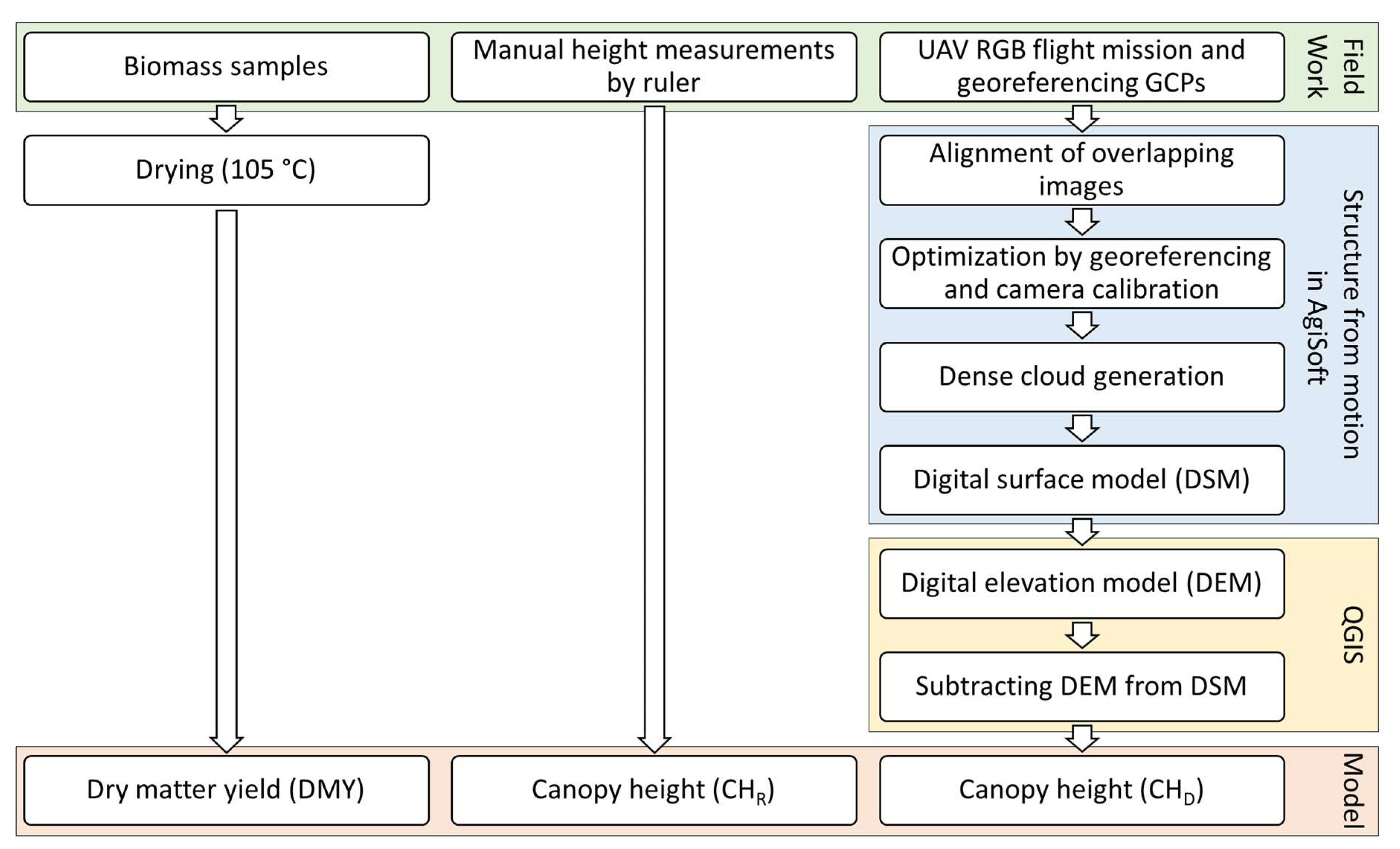
Three-dimensional (3D) point clouds were generated from the RGB images for each dataset using the SfM approach. The software Agisoft PhotoScan Professional (Agisoft LLC, St. Petersburg, Russia) was used to calculate the digital surface model (DSM) from the RGB images. The SfM algorithm obtains 3D information from 2D images and converts the images automatically into a DSM. All processing steps were executed separately for a better control, using uniform settings on a high-performance computer (Figure 2).
After importing a dataset, the overlapping images were aligned by internal image matching techniques and algorithms. Location and orientation of the individual images of the moving camera were automatically determined. The alignment was done with the accuracy setting “medium” and a key point limit of 40,000 and tie point limit of 4000. The output was a sparse point cloud containing a certain amount of paired multidimensional points of all images, which were linked together by identical features.
For the optimization step, the GPS coordinates of the GCPs were imported using the coordinate system WSG 84. The sparse point cloud was georeferenced manually by determining three pictures for each of the seven GCPs and placing the renumbered GCP marker on the cross center of the targets. After that, the software estimated the positions of the GCP marker for the other images automatically and, when needed, the markers were adjusted and placed manually. The spatial error of the GCPs varied between 1 and 2 cm. Additional optimizing of the sparse cloud was done by enhancing the camera lens parameters. With these optimized settings, the image alignment, the location and orientation of images and, eventually, the sparse point cloud was updated and corrected.
In the next step the georeferenced sparse point cloud was converted into a dense point cloud. The software computed the depth information by the image alignment for all points of the images. For that, medium quality settings were used to keep the processing time at an acceptable level and depth filtering was set to “aggressive” to sort out outlier points due to noise or inaccurate focusing. These steps resulted in one single point cloud, which was much denser and more detailed.
In the last step the dense point cloud was exported in the form of a DSM as a TIFF file with a resolution between 1 and 3 cm per pixel. The DSM represented the recorded surface as a raster data.
Further processing was done with Quantum Geographical Information System (QGIS 2.18.14, QGIS Development Team, Raleigh, NC, USA) software to provide a digital elevation model (DEM). After importing the raster image, ground points in the pathways next to the plots were selected from the DEM, which were interpolated by an inverse interpolation with a power of 3 to provide a continuous ground surface model over the whole field. CH was calculated by subtracting DEM from DSM. The coordinates of the plot corners were used to delimit each plot area. The mean height value for each plot from the drone-based RGB imaging (CHD) was extracted by zonal statistics. These processes were done for every flight mission separately. From the whole dataset seven CHD values had to be removed due to unrealistic negative height values.
2.4. Statistical Analysis
Statistical analysis was performed using R programming language version 3.5.1 (R Foundation for Statistical Computing, Vienna, Austria). DMY was tested for normal distribution and its residuals for homoscedasticity. As these assumptions were not fulfilled, DMY was square root transformed. ANOVA was used to detect differences among yields of the four cuts in each treatment.
For creating estimation models for the whole dataset (including the subsamples), CH and DMY were used for linear regression models. One main assumption for an ordinary least square (OLS) regression (Type-I regression model) is the allocation of y as dependent variable and x as independent variable. Another assumption for OLS is the measurement of the independent variable x without error. In our Study it was not feasible to distinguish between x and y for CH and DMY and as x (i.e., is CH) was measured both manually and by RGB imaging, the height measurements cannot be considered as error-free. In this case, a reduced major axis (RMA) regression, which is a Type-II regression model, was suggested by Cohen et al. [27] for analysis in the field of remote sensing. Though slope, intercept and root mean square error (RMSE) are calculated differently, RMA shows the same coefficient of determination (R2) as OLS. In the current study, RMA was used to predict DMY by CHR and CHD for the whole dataset and for the treatments separately. For a better understanding of the graphical presentation of the yield estimation model, the equations were re-transformed to the original scale.
For an assessment of the model accuracy, cross-validation was carried out. The dataset was split into a calibration (training) and validation dataset. To generate an even distribution of the randomly chosen validation dataset, one value was withdrawn from each treatment and sampling date, resulting in a 75% calibration and 25% validation dataset. The calibration dataset was used to generate the corresponding models and the coefficient of determination (R2cal), the root mean square error (RMSEcal) were calculated. The validation dataset was used as an independent dataset to verify the calibrated models by linear regression between measured and predicted DMY, represented by coefficient of determination (R2val) and root mean square error (RMSEval) as well as relative RMSEval (rRMSEval). Additionally, to determine the accuracy of the validation between measured and predicted DMY Willmott’s refined index of agreement (d) was generated. Willmott’s refined index of agreement is a dimensionless value between 0 and 1 indicating no agreement and total agreement, respectively [28].
3. Results
Ten datasets of DMY, CHR and CHD were collected throughout the vegetation period from May to October 2017. From the datasets of RGB images, which were processed by Agisoft PhotoScan into 3D models and further into CHD values, seven mean CHD values from the third and fourth sub-sampling, were negative and were, therefore, excluded from further analysis.
3.1. Dry Matter Yield
As the mixtures and pure stands were investigated at various growth stages throughout the growing season, DMY varied widely and declined in most cases with progressing growing season from first to fourth cut (Figure 3). DMY of pure grass swards exhibited a particularly strong decrease after the first cut. The mean DMY for the whole dataset including sub-samples ranged from 0.09 to 6.32 t ha−1 (Table A1).
3.2. Canopy Height
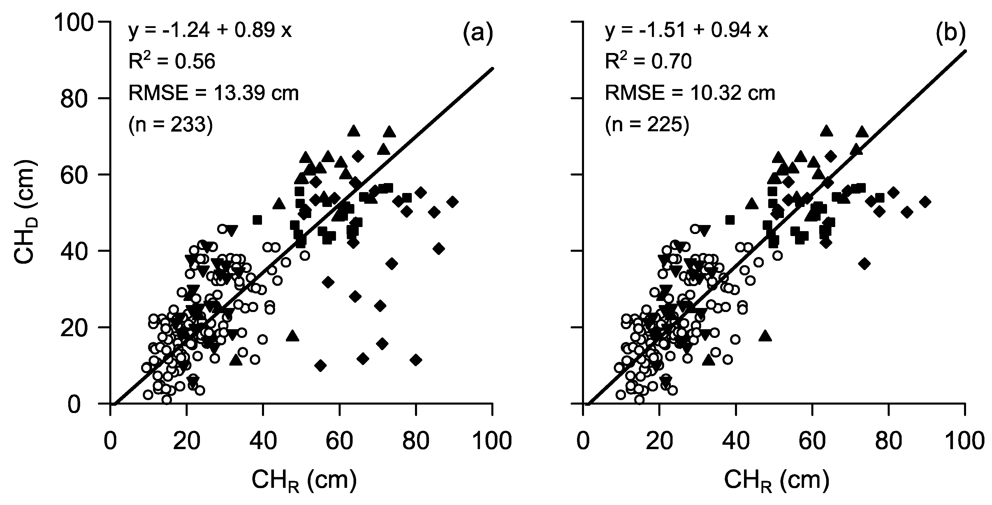
The average height values per treatment and date of CHR and CHD varied from 9.42 to 89.54 cm and 1.01 to 71.06 cm respectively (Figure 4a). On average, CHD was more than 4 cm lower than CHR. CH of sub-samplings and of the fourth cut were lower compared to the first, second and third cut. The linear relationship between CHR and CHD showed an R2 of 0.56 with an RMSE of 13.39 cm. CHR values of grass from the second cut were remarkably higher than the corresponding CHD values. If the data of the grass of the second cut were excluded from analysis, R2 and RMSE improved to 0.70 and 10.32 cm respectively (Figure 4b).
Considering the individual treatments, R2 for the mixtures and pure legume stands varied between 0.70 and 0.84 and rRMSE between 11 and 16% (Table 2). The pure grass treatments GCG and GLG showed a lower R2 of 0.47 (RMSE = 16.51 cm) and 0.29 (RMSE = 16.91 cm) respectively. Similarly to the complete dataset, when the second cut was also excluded from the analysis of the pure grass data, relationship between manual and UAV-based measurements were much better.
3.3. Prediction Models
CH as measured by ruler and UAV-based imaging was used as a predictor for DMY. Models were developed based on a calibration and validation dataset for the whole dataset as well as separately for the different treatments (Table 3). Regression analysis with the entire dataset and CHR as regressor resulted in an R2cal of 0.62 for calibration and an R2val of 0.64 for validation and a corresponding RMSEval of 0.28 t ha−1 (rRMSEval = 18%). Model performance for CHD was slightly better with R2cal = 0.69 and an R2val of 0.72 (rRMSE = 17%). Considering the individual treatments, R2cal varied between 0.58 and 0.80 and R2val between 0.42 and 0.68 (rRMSEval = 0.23–0.34 t ha−1) for CHR, while for CHD R2cal (R2cal = 0.62–0.80) and R2val (R2val = 0.46–0.87, rRMSEval = 0.23–0.36 t ha−1) was somewhat higher. Willmott’s refined index of agreement (d) of CHR and CHD varied on a similar high level between 0.82 and 0.92. Exclusion of the pure grass data of the second cut resulted in higher R2cal and R2val values, but only the rRMSEval values GGL of CHR (rRMSEval = 15%) and both grass treatments of CHD (rRMSEval = 16–19%) were lower. However, d yielded in a higher value for both, CHR and CHD by excluding pure grass data from the second cut (0.88–0.94).
A major aim of the study was to generate prediction models for DMY based on CHD, which are valid across the entire range of legume contribution possibly occurring in practical grassland farming (i.e., 0 to 100% of DMY). It turned out that models perform better when developed separately for the two legume species. Figure 5 shows the legume-specific linear models, each including the respective mixture as well as the corresponding pure legume and grass sward. For better understanding DMY data was re-transformed to the original scale. DMY of clover-grass was better predicted by CHD with an R2cal of 0.75 compared to CHR with R2cal of 0.60 (Table 4). Also the validation for clover-grass by CHD showed a higher R2val of 0.75 (rRMSEval = 17%) compared to CHR with an R2val of 0.58 (rRMSEval = 22%). In contrast, DMY of lucerne-grass was predicted and validation was performed somewhat better by CHR (R2cal = 0.67, R2val = 0.69) than by CHD (R2cal = 0.64, R2val = 0.62). The d value varied on a high level for all models between 0.87 and 0.93.
For practical implementation it is relevant to know the accuracy of the novel methodology for the prediction of the total annual DMY (ADMY), which is the total DMY of a crop over the entire growing season. In the present study ADMY was calculated by accumulating the harvest yield of all four cuts. ADMY varied between 11.85 and 15.18 t ha−1 for the whole dataset and the mixtures with a standard deviation (SD) between 2.01 and 2.37 (Table 5). By applying the prediction models (Table 4) and accumulating the estimated yields of the four cuts, estimates were produced for ADMY based on manual height measurement (ADMYR) as well as based on UAV-based RGB imaging (ADMYD) (Table 5). Similar results were predicted by CH measurement, which varied for ADMYR between 12.38 and 16.85 t ha−1 (SD = 1.92–2.17) and for ADMYD between 11.77 and 15.71 t ha−1 (SD = 1.76–2.62).
4. Discussion
The primary aim of this study was to develop and evaluate a prediction model for DMY of heterogeneous temperate grasslands by means of SfM using UAV-based RGB imaging. CH was successfully predicted both by manual and SfM height measurement. SfM-based CH was on average 4 cm lower than the manually measured values. The same tendency was found in previous studies with barley with a difference of 10 cm [17] and 19 cm [29], respectively, though both investigations used a higher resolution of 1 cm per pixel. In our study, manual measurements represented 50 single points from the ground soil to the highest point touching the ruler. In contrast, SfM datasets covered the whole area of interest, scanning the complete visible canopy surface and not only the top of single plants [17,19]. Furthermore, the nadir position of the camera with a resolution of 2 cm per pixel may not have captured every single grass tiller, especially at windy conditions, and the strong depth filtering during the generation of dense point clouds may have already caused an exclusion of single outlying points. All this led to a generally lower average CH compared to the manual measurements and is also supported by the finding that the correlation between SfM-based and manual height measurement improved, when the data of the extreme mature grasses of the second cut were excluded. Cunliffe et al. [30] showed that in dryland vegetation ultra-fine resolution of less than 1 cm of the height model was able to depict single grass stems.
The prediction models for DMY based on the calibration dataset of CHR and CHD showed similar accuracies across all treatments with R2 = 0.58–0.80 and R2 = 0.62–0.81, respectively. Most other multi-temporal studies reporting on SfM-based prediction models by means of UAV RGB imaging were conducted with arable crops. Correlation results were comparable for barley with an R2 = 0.82 [17], for winter wheat (R2 = 0.68–0.95) [16] and for maize and sorghum (R2 = 0.68–0.78) [31]. Moeckel et al. [20] achieved substantially higher R² values with stands of tomato, eggplant and cabbage (R2 = 0.89–0.97), which represent more heterogeneous crops. Roth and Streit [32] examined different cover crops, including also two clover species, and achieved an R2 of 0.58. When plants, which were growing close to the ground or even lodging, were excluded from the regression model, R2 increased to 0.74. In a permanent timothy-dominated grassland Viljanen et al. [25] obtained a pearson correlation coefficient between 0.77 and 0.97. They showed that the quality of the estimation model depended on plant density and growth stage of the sward. Bendig et al. [33] achieved the best results in summer barley prior to heading of the crop. Malambo et al. [31] and Grenzdörffer [34] showed that the SfM approach worked better for uniform crops than for crops with a heterogeneous canopy surface. Compared to other arable crops, which are usually grown in monocultures (e.g., cereals, maize), clover- and lucerne-grass mixtures form a rather heterogeneous canopy with a wide range of coverage of the two components, which above all, have a very different stature.
Several studies indicated that plant density influences the estimation of plant height [6,35,36]. In our study, the second cut was markedly affected by drought, which resulted particularly for grasses in a low tiller density and less leaf biomass. The exclusion of the data of the pure grass stands of the second cut improved the correlations for both methods. A camera with a higher resolution to capture more details of the canopy surface [30] and the integration of plant density as additional information may further improve the prediction accuracy in heterogeneous crops. In a study of Schut et al. [37] the combination of spectral indices with remotely sensed CH information showed promising results at small-scaled farm level. In other studies fusion of 3D LiDAR and spectral data substantially improved biomass prediction in extensively manage permanent grasslands compared to the use of single sensors [5,12].
Accuracy of biomass estimation by RGB imaging may be reduced due to errors and uncertainties during the image and point cloud generation. The seven negative CHD values, which were excluded from the present analysis, were located in an area of the experimental site, where a slight slope occurred. In our study, the DEM was generated by the interpolation of z-values from points located in the pathways between the plots. As the biomass at the erased points were extremely low, negative height values may, thus, have been caused by an inadequate representation of the true ground surface in the interior of the plots. With a small and rather flat area like our experimental field the error due to insufficient interpolation is relatively low, whereas for practical and possibly uneven fields of several hectares explicitly generated DEM point clouds may be necessary for a sound calculation of canopy heights. This can e.g., be done during periods of bare soil, e.g., before sowing or after harvest of the crop. However, the production of additional pre-sowing or post-harvest point clouds requires extra flight missions and a considerable effort of data analysis. Tests which were conducted prior to the experiment indicated that extremely diligent georeferencing of the point clouds with an adequate number of georeferenced control points is necessary to avoid errors and uncertainties in the CH data.
In practical forage production strategic decisions (e.g., for adjusting the number of farm animals to the amount of available roughage) are usually taken based on data from one year or growing season. Thus, generating reliable data on the expected total annual biomass produced from single fields would substantially support farmers’ decisions. As a first approach models were developed to predict total annual yield separately for the clover- and lucerne-grass stands. As the legume contribution of legume-grass mixtures varies greatly in farming practice [38], the corresponding pure stands of legumes and grasses were also included in both models. The fact, that model accuracy was different for clover- (R2 = 0.75) and lucerne-grass (R2 = 0.64) data indicates that, morphological characteristics (e.g., leaf position, vertical or horizontal distribution) of clover canopies allow a better prediction of biomass than for lucerne-grass mixtures, and that these crop-specific models cannot be easily transferred to other grassland types. The reasons behind this finding cannot be determined with the present study and, thus, further investigations (also considering model evaluation on the field scale) are needed. However, it is encouraging that averaged across all treatments, the accuracy between measured yield and UAV-based yield assessment was similar to manual height measurement.
Data acquisition by UAV can be done in a relative short time, whereas data processing by SfM is a computationally intensive process, depending on computer performance and number of images. In our study, data acquisition for each sampling date by manual height measurement, which was a rather high number of measurements (50 measurements per plot ~ 3 h) and UAV-based RGB imaging including data processing yielded in a similar amount of time (~ 3–4 h). So far, a practical implementation does not seem feasible, but as flight time of UAVs, computer performance and automation of data processing steadily increases, this method is seen to have great potential. To summarize, the results indicate that UAV-based RGB imaging may serve as a suitable estimator for total annual yield of heterogeneous legume-grass mixtures, which future studies should evaluate.
5. Conclusions
Accurate yield estimation in temporal grassland farming is an essential prerequisite for management decisions. The present study showed, that SfM-based RGB imaging in combination with a UAV provides a promising alternative to the time- and effort-consuming yield prediction based on conventional manual methods. Furthermore, yield estimation by RGB imaging proved similar prediction of DMY at extreme weather conditions compared to manual height measurements by ruler. Our new approach to yield assessment by SfM showed great potential and was also able to successfully estimate total annual yield. The use of UAVs serves as a fast, non-destructive tool for multi-temporal data acquisition.
However, the large variability of canopy surface in legume-grass mixtures causes lower prediction accuracies than in more homogeneous arable crops. Therefore, instead of using single sensors, research should focus on fusion of complementary sensor data, e.g., by including spatial and spectral information. The fast-emerging technologies in remote sensing have a great potential to develop such sensor systems integrated on one UAV platform.
Author Contributions
T.A. and M.W. conceived the idea of the study. E.G., conducted the field work, processed and analyzed the data and wrote the manuscript. T.A. assisted in field work and statistical analysis. T.A. and M.W. supervised the work, contributed to the interpretation of the results and revised the text.
Acknowledgments
The authors would like to thank Wolfgang Funke for his support in field data collection and Rüdiger Graß for advice in crop management.
Conflicts of Interest
The authors declare no conflict of interest. The funders had no role in the design of the study; in the collection, analyses, or interpretation of data; in the writing of the manuscript, and in the decision to publish the results.
Appendix A

Table A1.
Dry matter yield (DMY) of the different treatments: the clover-grass (CG) and lucerne-grass (LG) mixtures and pure stands of legumes (L) and grasses (G) for 10 sampling dates comprising four harvest cuts and six sub-samplings every second week during sward growth between 17 May 2017 and 9 October 2017.
| Cut Date | DMY (t ha−1) | |||||||||
|---|---|---|---|---|---|---|---|---|---|---|
| 1st harvest | 1st sub-sample | 2nd sub-sample | 2nd harvest | 3rd sub-sample | 3rd harvest | 4th sub-sample | 5th sub-sample | 6th sub-sample | 4th harvest | |
| 17 May 2017 | 2 June 2017 | 13 June 2017 | 26 June 2017 | 11 July 2017 | 8 August 2017 | 23 August 2017 | 5 September 2017 | 20 September 2017 | 9 October 2017 | |
| Treatment | ||||||||||
| CG | 4.60 | 0.78 | 2.29 | 3.40 | 0.73 | 4.82 | 0.44 | 1.15 | 1.79 | 2.37 |
| LG | 4.90 | 0.60 | 2.21 | 3.47 | 0.67 | 2.57 | 0.78 | 1.70 | 1.87 | 1.95 |
| LCG | 4.95 | 0.35 | 1.49 | 1.97 | 0.29 | 0.74 | 0.33 | 0.87 | 1.35 | 1.17 |
| LLG | 3.59 | 1.12 | 2.59 | 3.79 | 1.03 | 3.53 | 0.78 | 2.06 | 2.93 | 2.46 |
| GCG | 4.58 | 0.57 | 1.59 | 1.62 | 0.21 | 0.66 | 0.41 | 0.86 | 1.08 | 1.05 |
| GLG | 3.41 | 0.76 | 1.97 | 3.53 | 0.95 | 3.33 | 0.52 | 1.81 | 1.81 | 2.70 |
References
- Sanderson, M.A.; Rotz, C.A.; Fultz, S.W.; Rayburn, E.B. Estimating Forage Mass with a Commercial Capacitance Meter, Rising Plate Meter, and Pasture Ruler. Agron. J. 2001, 93, 1281. [Google Scholar] [CrossRef]
- Schellberg, J.; Hill, M.J.; Gerhards, R.; Rothmund, M.; Braun, M. Precision agriculture on grassland: Applications, perspectives and constraints. Eur. J. Agron. 2008, 29, 59–71. [Google Scholar] [CrossRef]
- Wachendorf, M.; Fricke, T.; Möckel, T. Remote sensing as a tool to assess botanical composition, structure, quantity and quality of temperate grasslands. Grass Forage Sci. 2017, 35, 201. [Google Scholar] [CrossRef]
- Catchpole, E.R.; Wheeler, C.J. Estimating plant biomass: A review of techniques. Aust. J. Ecol. 1992, 121–131. [Google Scholar] [CrossRef]
- Fricke, T.; Wachendorf, M. Combining ultrasonic sward height and spectral signatures to assess the biomass of legume–grass swards. Comput. Electron. Agric. 2013, 99, 236–247. [Google Scholar] [CrossRef]
- Holman, F.; Riche, A.; Michalski, A.; Castle, M.; Wooster, M.; Hawkesford, M. High Throughput Field Phenotyping of Wheat Plant Height and Growth Rate in Field Plot Trials Using UAV Based Remote Sensing. Remote Sens. 2016, 8, 1031. [Google Scholar] [CrossRef]
- Hakl, J.; Hrevušová, Z.; Hejcman, M.; Fuksa, P. The use of a rising plate meter to evaluate lucerne (Medicago sativa L.) height as an important agronomic trait enabling yield estimation. Grass Forage Sci. 2012, 67, 589–596. [Google Scholar] [CrossRef]
- Ondřej, C.; Josef, H.; Michal, H.; Pavel, C. The use of compressed height to estimate the yield of a differently fertilized meadow. Plant Soil Environ. 2018, 64, 76–81. [Google Scholar] [CrossRef] [Green Version]
- Harmoney, K.R.; Moore, K.J.; George, J.R.; Brummer, E.C.; Russell, J.R. Determination of Pasture Biomass Using Four Indirect Methods. Agron. J. 1997, 89, 665. [Google Scholar] [CrossRef]
- Künnemeyer, R.; Schaare, P.N.; Hanna, M.M. A simple reflectometer for on-farm pasture assessment. Comput. Electron. Agric. 2001, 31, 125–136. [Google Scholar] [CrossRef]
- Lu, D. The potential and challenge of remote sensing-based biomass estimation. Int. J. Remote Sens. 2006, 27, 1297–1328. [Google Scholar] [CrossRef]
- Moeckel, T.; Safari, H.; Reddersen, B.; Fricke, T.; Wachendorf, M. Fusion of Ultrasonic and Spectral Sensor Data for Improving the Estimation of Biomass in Grasslands with Heterogeneous Sward Structure. Remote Sens. 2017, 9, 98. [Google Scholar] [CrossRef]
- Wallace, L.; Hillman, S.; Reinke, K.; Hally, B.; Kriticos, D. Non-destructive estimation of above-ground surface and near-surface biomass using 3D terrestrial remote sensing techniques. Methods Ecol. Evol. 2017, 257, 1684. [Google Scholar] [CrossRef]
- Forsmoo, J.; Anderson, K.; Macleod, C.J.A.; Wilkinson, M.E.; Brazier, R.; Smit, I. Drone-based structure-from-motion photogrammetry captures grassland sward height variability. J. Appl. Ecol. 2018, 94, 237. [Google Scholar] [CrossRef]
- Dittmann, S.; Thiessen, E.; Hartung, E. Applicability of different non-invasive methods for tree mass estimation: A review. For. Ecol. Manag. 2017, 398, 208–215. [Google Scholar] [CrossRef]
- Schirrmann, M.; Giebel, A.; Gleiniger, F.; Pflanz, M.; Lentschke, J.; Dammer, K.-H. Monitoring Agronomic Parameters of Winter Wheat Crops with Low-Cost UAV Imagery. Remote Sens. 2016, 8, 706. [Google Scholar] [CrossRef]
- Bendig, J.; Bolten, A.; Bennertz, S.; Broscheit, J.; Eichfuss, S.; Bareth, G. Estimating Biomass of Barley Using Crop Surface Models (CSMs) Derived from UAV-Based RGB Imaging. Remote Sens. 2014, 6, 10395–10412. [Google Scholar] [CrossRef] [Green Version]
- Geipel, J.; Link, J.; Claupein, W. Combined Spectral and Spatial Modeling of Corn Yield Based on Aerial Images and Crop Surface Models Acquired with an Unmanned Aircraft System. Remote Sens. 2014, 6, 10335–10355. [Google Scholar] [CrossRef] [Green Version]
- Li, W.; Niu, Z.; Chen, H.; Li, D.; Wu, M.; Zhao, W. Remote estimation of canopy height and aboveground biomass of maize using high-resolution stereo images from a low-cost unmanned aerial vehicle system. Ecol. Indic. 2016, 67, 637–648. [Google Scholar] [CrossRef]
- Moeckel, T.; Dayananda, S.; Nidamanuri, R.; Nautiyal, S.; Hanumaiah, N.; Buerkert, A.; Wachendorf, M. Estimation of Vegetable Crop Parameter by Multi-temporal UAV-Borne Images. Remote Sens. 2018, 10, 805. [Google Scholar] [CrossRef]
- Ergon, Å.; Kirwan, L.; Bleken, M.A.; Skjelvåg, A.O.; Collins, R.P.; Rognli, O.A. Species interactions in a grassland mixture under low nitrogen fertilization and two cutting frequencies: 1. dry-matter yield and dynamics of species composition. Grass Forage Sci. 2016, 71, 667–682. [Google Scholar] [CrossRef] [Green Version]
- Elgersma, A.; Søegaard, K. Changes in nutritive value and herbage yield during extended growth intervals in grass-legume mixtures: Effects of species, maturity at harvest, and relationships between productivity and components of feed quality. Grass Forage Sci. 2018, 73, 78–93. [Google Scholar] [CrossRef]
- Cooper, S.; Roy, D.; Schaaf, C.; Paynter, I. Examination of the Potential of Terrestrial Laser Scanning and Structure-from-Motion Photogrammetry for Rapid Nondestructive Field Measurement of Grass Biomass. Remote Sens. 2017, 9, 531. [Google Scholar] [CrossRef]
- Van Iersel, W.; Straatsma, M.; Addink, E.; Middelkoop, H. Monitoring height and greenness of non-woody floodplain vegetation with UAV time series. ISPRS J. Photogramm. Remote Sens. 2018, 141, 112–123. [Google Scholar] [CrossRef]
- Viljanen, N.; Honkavaara, E.; Näsi, R.; Hakala, T.; Niemeläinen, O.; Kaivosoja, J. A Novel Machine Learning Method for Estimating Biomass of Grass Swards Using a Photogrammetric Canopy Height Model, Images and Vegetation Indices Captured by a Drone. Agriculture 2018, 8, 70. [Google Scholar] [CrossRef]
- Heady, H.F. The Measurement and Value of Plant Height in the Study of Herbaceous Vegetation. Ecology 1957, 38, 313–320. [Google Scholar] [CrossRef]
- Cohen, W.B.; Maiersperger, T.K.; Gower, S.T.; Turner, D.P. An improved strategy for regression of biophysical variables and Landsat ETM+ data. Remote Sens. Environ. 2003, 84, 561–571. [Google Scholar] [CrossRef] [Green Version]
- Willmott, C.J. On the validation of models. Phys. Geogr. 1981, 184–194. [Google Scholar] [CrossRef]
- Aasen, H.; Burkart, A.; Bolten, A.; Bareth, G. Generating 3D hyperspectral information with lightweight UAV snapshot cameras for vegetation monitoring: From camera calibration to quality assurance. ISPRS J. Photogramm. Remote Sens. 2015, 108, 245–259. [Google Scholar] [CrossRef]
- Cunliffe, A.M.; Brazier, R.E.; Anderson, K. Ultra-fine grain landscape-scale quantification of dryland vegetation structure with drone-acquired structure-from-motion photogrammetry. Remote Sens. Environ. 2016, 183, 129–143. [Google Scholar] [CrossRef] [Green Version]
- Malambo, L.; Popescu, S.C.; Murray, S.C.; Putman, E.; Pugh, N.A.; Horne, D.W.; Richardson, G.; Sheridan, R.; Rooney, W.L.; Avant, R.; et al. Multitemporal field-based plant height estimation using 3D point clouds generated from small unmanned aerial systems high-resolution imagery. Int. J. Appl. Earth Obs. Geoinf. 2018, 64, 31–42. [Google Scholar] [CrossRef]
- Roth, L.; Streit, B. Predicting cover crop biomass by lightweight UAS-based RGB and NIR photography: An applied photogrammetric approach. Precis. Agric. 2018, 19, 93–114. [Google Scholar] [CrossRef]
- Bendig, J.; Yu, K.; Aasen, H.; Bolten, A.; Bennertz, S.; Broscheit, J.; Gnyp, M.L.; Bareth, G. Combining UAV-based plant height from crop surface models, visible, and near infrared vegetation indices for biomass monitoring in barley. Int. J. Appl. Earth Obs. Geoinf. 2015, 39, 79–87. [Google Scholar] [CrossRef]
- Grenzdörffer, G.J. Crop height determination with UAS point clouds. Int. Arch. Photogramm. Remote Sens. Spat. Inf. Sci. 2014, XL-1, 135–140. [Google Scholar] [CrossRef]
- Gillan, J.K.; Karl, J.W.; Duniway, M.; Elaksher, A. Modeling vegetation heights from high resolution stereo aerial photography: An application for broad-scale rangeland monitoring. J. Environ. Manag. 2014, 144, 226–235. [Google Scholar] [CrossRef] [PubMed]
- Watanabe, K.; Guo, W.; Arai, K.; Takanashi, H.; Kajiya-Kanegae, H.; Kobayashi, M.; Yano, K.; Tokunaga, T.; Fujiwara, T.; Tsutsumi, N.; et al. High-Throughput Phenotyping of Sorghum Plant Height Using an Unmanned Aerial Vehicle and Its Application to Genomic Prediction Modeling. Front. Plant Sci. 2017, 8, 421. [Google Scholar] [CrossRef] [PubMed]
- Schut, A.G.T.; Traore, P.C.S.; Blaes, X.; de By, R.A. Assessing yield and fertilizer response in heterogeneous smallholder fields with UAVs and satellites. Field Crop. Res. 2018, 221, 98–107. [Google Scholar] [CrossRef]
- Ledgard, S.F.; Steele, K.W. Biological nitrogen fixation in mixed legume/grass pastures. Plant Soil 1992, 141, 137–153. [Google Scholar] [CrossRef]
Figure 1.
(A) Germany’s political map showing the location of Hesse; (B) North-Hesse’s political map showing the location of the experimental site in Neu-Eichenberg; (C) Orthomosaic of the experimental field showing the different plots on 7 August 2017, at the time of the third cut.
Figure 1.
(A) Germany’s political map showing the location of Hesse; (B) North-Hesse’s political map showing the location of the experimental site in Neu-Eichenberg; (C) Orthomosaic of the experimental field showing the different plots on 7 August 2017, at the time of the third cut.

Figure 2.
Workflow of biomass sampling, manual and UAV-based structure from motion (SfM) height measurement.
Figure 2.
Workflow of biomass sampling, manual and UAV-based structure from motion (SfM) height measurement.

Figure 3.
Dry matter yield (DMY) at four cuts of clover-grass (CG, left) and lucerne-grass (LG, right) mixtures (a,d) as well as pure stands of legumes (L) (b,e) and grasses (G) (c, f). *** = p < 0.001; * = p < 0.05; n.s. = not significant.
Figure 3.
Dry matter yield (DMY) at four cuts of clover-grass (CG, left) and lucerne-grass (LG, right) mixtures (a,d) as well as pure stands of legumes (L) (b,e) and grasses (G) (c, f). *** = p < 0.001; * = p < 0.05; n.s. = not significant.
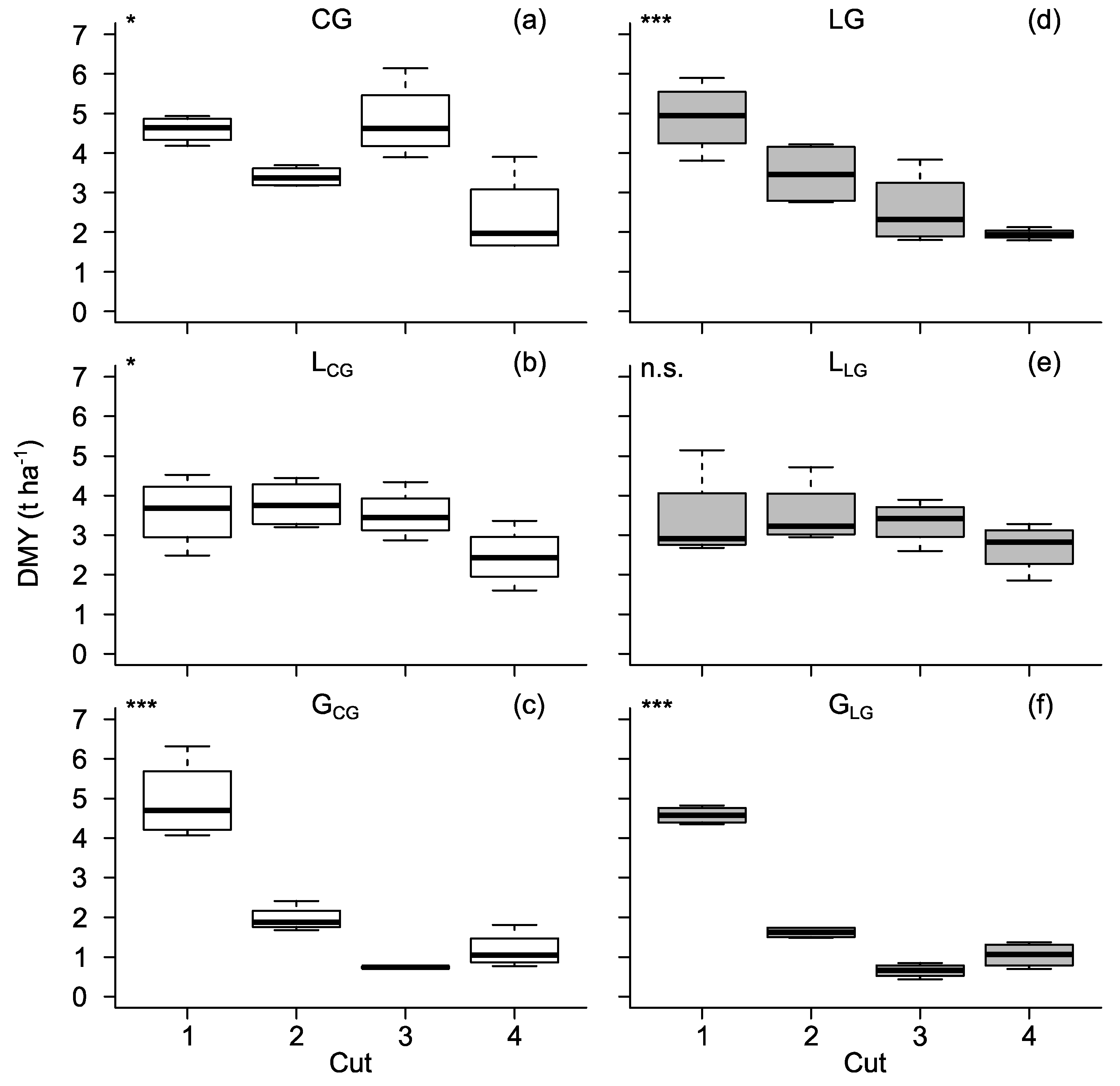
Figure 4.
Linear relationship between canopy height from manual height measurements (CHR) and UAV-based RGB imaging (CHD) for the whole dataset (a) and for the whole dataset excluding pure grass stands of the second cut (b). The different symbols indicate sub-samples (○), which were taken between the first (■), second (◆), third (▲) and fourth (▼) harvest.

Figure 5.
Legume-specific regression models of the calibration dataset with validation dataset (●) for dry matter yield (DMY) based on canopy height from UAV-based RGB imaging (CHD). For better understanding DMY data was re-transformed to the original scale. Models for clover-grass (a) and lucerne-grass (b) both include the respective mixtures as well as the corresponding pure legume and grass swards. R2 = coefficient of determination; rRMSE = relative root mean square error (calculated with square root-transformed data).
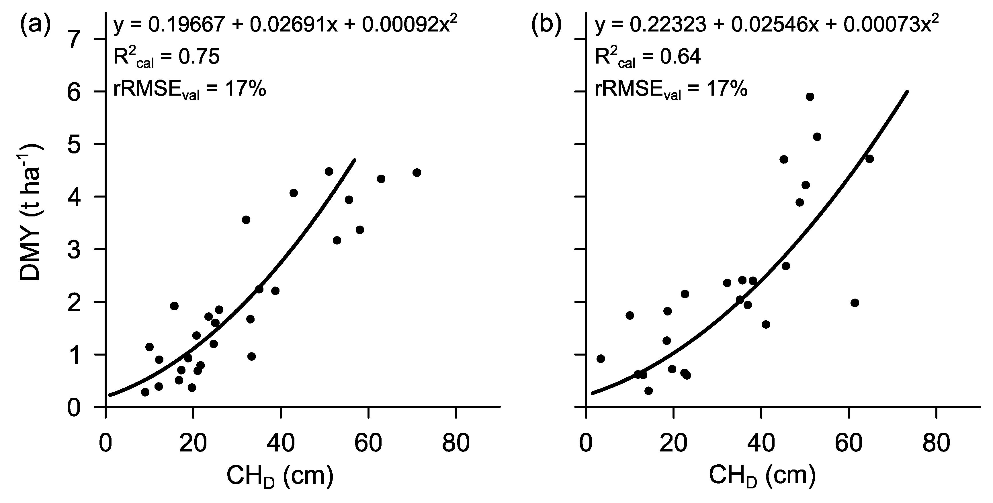
Table 1.
List of the treatments with functional groups, species and their ratio in the seed mixture of each treatment.
Table 1.
List of the treatments with functional groups, species and their ratio in the seed mixture of each treatment.
| Treatment | Functional Group | Species | Ratio (%) | |
|---|---|---|---|---|
| Clover-grass mixture | CG | Legumes (L) | Trifolium pratense Trifolium hybridum Trifolium repens | 30 5 5 |
| Grass (G) | Lolium multiflorum | 60 | ||
| Lucerne-grass mixture | LG | L | Medicago sativa Trifolium pratense | 40 10 |
| G | Festuca pratensis Lolium perenne Lolium multiflorum Phleum pratense | 20 15 10 5 | ||
| Pure clover legumes | LCG | L from CG mixture | Trifolium pratense Trifolium hybridum Trifolium repens | 75 12.5 12.5 |
| Pure lucerne and clover legumes | LLG | L from LG mixture | Medicago sativa Trifolium pratense | 80 20 |
| Pure grass sward | GCG | G from CG mixture | Lolium multiflorum | 100 |
| Pure grass sward | GLG | G from LG mixture | Festuca pratensis Lolium perenne Lolium multiflorum Phleum pratense | 40 30 20 10 |
CG = clover-grass; LG = lucerne-grass.
Table 2.
Coefficients of determination (R2), root mean square errors (RMSE) and relative RMSE (rRMSE) of linear regression analysis between manual height measurements (CHR) and UAV-based RGB imaging (CHD) for the whole dataset (All) and the different treatments: clover-grass (CG), lucerne-grass (LG) as well as the pure stands of legumes (LCG, LLG) and grass (GCG, GLG) of the mixtures, respectively. Values in brackets represent results for the dataset without pure grass swards of the second cut.
| Treatment | R2 | RMSE (cm) | rRMSE (%) |
|---|---|---|---|
| All | 0.56 (0.70) | 13.39 (10.32) | 17 (13) |
| CG | 0.79 | 10.19 | 13 |
| LG | 0.70 | 11.14 | 16 |
| LCG | 0.84 | 6.08 | 11 |
| LLG | 0.72 | 8.70 | 16 |
| GCG | 0.47 (0.70) | 16.51 (9.17) | 22 (14) |
| GLG | 0.29 (0.57) | 16.91 (9.35) | 24 (17) |
Table 3.
Linear regression analysis of calibration (cal) and validation (val) dataset between dry matter yield and manual height measurements (CHR) as well as UAV-based RGB imaging (CHD) for the whole dataset (All) and the different treatments: clover-grass (CG), lucerne-grass (LG) as well as the pure stands of legumes (LCG, LLG) and grass (GCG, GLG) of the mixtures, respectively. n = number of samples; R2 = coefficient of determination; RMSE = root mean square error; rRMSE = relative RMSE; d = Willmott’s refined index of agreement. Values in brackets represent results for the dataset without pure grass swards of the second cut.
| Treatment | Calibration | Validation | |||||
|---|---|---|---|---|---|---|---|
| ncal | R2cal | nval | R2val | RMSEval (t ha−1) | rRMSEval (%) | d | |
| CHR | |||||||
| All | 180 (174) | 0.62 (0.71) | 53 (51) | 0.64 (0.65) | 0.28 (0.29) | 18 (19) | 0.90 (0.90) |
| CG | 30 | 0.80 | 10 | 0.66 | 0.34 | 19 | 0.90 |
| LG | 30 | 0.71 | 9 | 0.50 | 0.33 | 19 | 0.85 |
| LCG | 30 | 0.68 | 10 | 0.56 | 0.26 | 21 | 0.87 |
| LLG | 30 | 0.77 | 8 | 0.68 | 0.23 | 19 | 0.91 |
| GCG | 30 (27) | 0.64 (0.82) | 8 (7) | 0.42 (0.51) | 0.33 (0.34) | 21 (22) | 0.83 (0.88) |
| GLG | 30 (27) | 0.58 (0.82) | 8 (7) | 0.43 (0.73) | 0.29 (0.20) | 22 (15) | 0.82 (0.94) |
| CHD | |||||||
| All | 180 (174) | 0.69 (0.73) | 53 (51) | 0.72 (0.62) | 0.27 (0.30) | 17 (20) | 0.92 (0.89) |
| CG | 30 | 0.80 | 10 | 0.87 | 0.23 | 13 | 0.96 |
| LG | 30 | 0.63 | 9 | 0.68 | 0.35 | 20 | 0.89 |
| LCG | 30 | 0.81 | 10 | 0.46 | 0.29 | 24 | 0.83 |
| LLG | 30 | 0.62 | 8 | 0.51 | 0.36 | 30 | 0.82 |
| GCG | 30 (27) | 0.68 (0.69) | 8 (7) | 0.54 (0.64) | 0.35 (0.30) | 23 (19) | 0.85 (0.90) |
| GLG | 30 (27) | 0.67 (0.71) | 8 (7) | 0.48 (0.77) | 0.30 (0.20) | 23 (16) | 0.86 (0.94) |
Table 4.
Linear regression analysis of calibration (cal) and validation (val) dataset between dry matter yield and manual height measurements (CHR) as well as UAV-based RGB imaging (CHD) for clover-grass (CG) and lucerne-grass (LG) mixtures including corresponding pure stands of legumes (L) and grass swards (G). n = number of samples; R2 = coefficient of determination; RMSE = root mean square error; rRMSE = relative RMSE; d = Willmott’s refined index of agreement.
| Treatment | Calibration | Validation | |||||
|---|---|---|---|---|---|---|---|
| ncal | R2cal | nval | R2val | RMSEval (t ha−1) | rRMSEval (%) | d | |
| CHR | |||||||
| Clover-grass (CG, LCG, GCG) Lucerne-grass (LG, LLG, GLG) | 90 | 0.60 | 28 | 0.58 | 0.34 | 22 | 0.87 |
| 90 | 0.65 | 25 | 0.69 | 0.29 | 16 | 0.90 | |
| CHD | |||||||
| Clover-grass (CG, LCG, GCG) Lucerne-grass (LG, LLG, GLG) | 90 | 0.75 | 28 | 0.75 | 0.26 | 17 | 0.93 |
| 90 | 0.64 | 25 | 0.62 | 0.32 | 17 | 0.88 | |
Table 5.
Measured total annual dry matter yield including four cuts (ADMY) and the predicted ADMY based on manual height measurement (ADMYR) and UAV-based RGB imaging (ADMYD) for the whole dataset (All) and the two different mixtures clover-grass (CG) and lucerne-grass (LG). For better understanding DMY data was re-transformed to the original scale. SD = standard deviation.
| Treatment | ADMY (t ha−1) | ADMYR (t ha−1) | ADMYD (t ha−1) | |||
|---|---|---|---|---|---|---|
| Mean | SD | Mean | SD | Mean | SD | |
| All | 11.85 | 2.01 | 12.38 | 1.92 | 11.77 | 2.09 |
| CG | 15.18 | 2.25 | 16.85 | 2.14 | 15.71 | 2.62 |
| LG | 12.88 | 2.37 | 13.73 | 2.17 | 12.30 | 1.76 |
© 2019 by the authors. Licensee MDPI, Basel, Switzerland. This article is an open access article distributed under the terms and conditions of the Creative Commons Attribution (CC BY) license (http://creativecommons.org/licenses/by/4.0/).
Share and Cite
MDPI and ACS Style
Grüner, E.; Astor, T.; Wachendorf, M. Biomass Prediction of Heterogeneous Temperate Grasslands Using an SfM Approach Based on UAV Imaging. Agronomy 2019, 9, 54. https://0-doi-org.brum.beds.ac.uk/10.3390/agronomy9020054
AMA Style
Grüner E, Astor T, Wachendorf M. Biomass Prediction of Heterogeneous Temperate Grasslands Using an SfM Approach Based on UAV Imaging. Agronomy. 2019; 9(2):54. https://0-doi-org.brum.beds.ac.uk/10.3390/agronomy9020054
Chicago/Turabian StyleGrüner, Esther, Thomas Astor, and Michael Wachendorf. 2019. "Biomass Prediction of Heterogeneous Temperate Grasslands Using an SfM Approach Based on UAV Imaging" Agronomy 9, no. 2: 54. https://0-doi-org.brum.beds.ac.uk/10.3390/agronomy9020054
Note that from the first issue of 2016, this journal uses article numbers instead of page numbers. See further details here.