Upscaling Evapotranspiration with Parsimonious Models in a North Carolina Vineyard


1
National Laboratory for Agriculture and the Environment, USDA-ARS, Ames, IA 50011, USA
2
Crop and Soil Sciences, North Carolina State University, Raleigh, NC 27695, USA
3
Los Lunas Agricultural Science Center, New Mexico State University, Los Lunas, NM 87031, USA
*
Author to whom correspondence should be addressed.
Agronomy 2019, 9(3), 152; https://0-doi-org.brum.beds.ac.uk/10.3390/agronomy9030152
Submission received: 11 February 2019
/
Revised: 16 March 2019
/
Accepted: 19 March 2019
/
Published: 23 March 2019
Abstract
:Water stress can positively or negatively impact grape yield and yield quality, and there is a need for wine growers to accurately regulate water use. In a four-year study (2010–2013), energy balance fluxes were measured with an eddy-covariance (EC) system in a North Carolina vineyard (Vitis vinifera cv. Chardonnay), and evapotranspiration (ET) and the Crop Water Stress Index (CWSI) calculated. A multiple linear regression model was developed to upscale ET using air temperature (Ta), vapor pressure deficit (VPD), and Landsat-derived Land Surface Temperature (LST) and Enhanced Vegetation Index (EVI). Daily ET reached values of up to 7.7 mm day−1, and the annual ET was 752 ± 59 mm, as measured with the EC system. The grapevine CWSI was between 0.53–0.85, which indicated moderate water stress levels. Median vineyard EVI was between 0.22 and 0.72, and the EVI range (max–min) within the vineyard was 0.18. The empirical models explained 75%–84% of the variation in ET, and all parameters had a positive linear relationship to ET. The Root Mean Square Error (RMSE) was 0.52–0.62 mm. This study presents easily applicable approaches to analyzing water dynamics and ET. This may help wine growers to cost-effectively quantify water use in vineyards.
1. Introduction
Quantifying water use in a vineyard is critical because plant available water in the root zone determines yield quantity and quality. The vines require no-stress conditions from bud break subsequent to fruit set, while moderate water stress is required during fruit ripening. Moderate water stress has an inhibitive effect on vegetative growth, which can enhance or positively impact berry composition, and eventually wine quality. Depending on the grapevine phenological stage, excessive water stress or oversupply of water can negatively impact yield and quality [1]. Water use in vineyards can be regulated by estimating the daily actual evapotranspiration (ET), i.e., the amount of water transpired by the crop, or evaporated from the soil and exposed surfaces. The goal in semi-arid wine regions is to reduce ET [2,3,4], however, wine growers in North Carolina (NC) and other humid regions seek to increase ET to a maximum because the high annual precipitation (P) inhibits vines to enter any water stress period during fruit ripening. A variety of techniques have been used to estimate ET in vineyards. Estimating latent heat flux (LE) using the Eddy covariance (EC) method has the advantage of generating continuous long-term ET datasets in vineyards on a sub-field or field level [5].
The Estimated Crop Water Stress Index (CWSI) is another method of quantifying plant water stress based on canopy temperature (Tc) measurements [6,7]. CWSI is related to the ratio of ET and potential ET (ETp) [7]:
The ET and Tc are related, because evaporative cooling of a transpiring plant reduces Tc, and water stressed plants close their stomates reducing ET, which leads to increased Tc. Several studies have successfully utilized the CWSI approach to quantify water stress [8,9]. More recently, the CWSI was applied in vineyards to map vine water stress and demonstrated that CWSI was related to stem water potential and yield parameters in grapevines [10,11,12,13].
There is a growing demand to cost-effectively quantify ET for whole vineyards. Previous studies used different modelling approaches or included remotely sensed data to estimate large-scale ET. One approach was the use of air-borne measured land surface temperature (LST) and air temperature (Ta) to estimate sensible heat (H). The LE and ET were then calculated as the residual energy in the energy balance equation [14]. Applying this concept, models for large-scale ET estimations have been developed. The Surface Energy Balance Algorithm for Land (SEBAL) estimates H using LST on very wet and dry conditions, i.e., at potential and zero LE [15]. A similar approach is the Mapping Evapotranspiration with Internalized Calibration (METRIC), which combines the SEBAL approach with micro-meteorological measurements on the ground [16]. The METRIC model was used to estimate regional vineyard ET in Chile in comparison with EC measurements [2]. The Simplified Surface Energy Balance Index (S-SEBI) model [17], another energy balance model based on LST, had previously been utilized to simulate ET in a vineyard in the Mediterranean region [4]. The Alexi/Disalexi approach uses a two-source energy balance (TSEB) model together with satellite-derived Normalized Difference Vegetation Index (NDVI), LST, and other meteorological data in a data fusion method to create daily ET products [3,18]. This approach was used for tempo-spatial estimation of ET in different agroecosystems, such as in vineyards in California [3,18]. More methods of ET estimation have been described in the literature [19].
While these modeling approaches are well developed to estimate ET, a more parsimonious model to upscale ET from sub-field ground measurements to total production areas is more accessible to growers. Volumetric soil water content (VWC) as a predictor of ET, and measured with EC stations, was used to upscale ET in the North American monsoon region [20]. Another way to estimate ET was the use of the reference evapotranspiration (ET0) multiplied with a crop coefficient (kc) [21], of which the former was calculated from meteorological data, and the latter was substituted by a satellite-derived vegetation index (VI) [14,22]. In addition, [23] reported that substituting ET0 with Ta showed good agreement in upscaling ET, using a simple empirical model with the Enhanced Vegetation Index (EVI) as a kc substitute in riparian vegetation in the Southwest U.S. Other climatic variables may also be used to substitute ET0. Landsat imagery provides EVI and LST products at a 30 × 30 m resolution, which would allow ET to be estimated on a subfield level using parsimonious regression models.
In this four-year study, actual ET and CWSI were estimated in a commercial vineyard in NC, USA, using the EC method as a comparison to quantify associated ET. This study’s aim was to monitor the water dynamics and quantify ET, and to eventually upscale ET from sub-field to vineyard level by developing a parsimonious empirical model using micro-meteorological data and Landsat 7 imagery.
2. Materials and Methods
2.1. Study Site
The study was conducted from April 2010 to November 2013 at a commercial vineyard (~8.7 ha) near Dobson, NC (−80.777° W; 36.357° N; 366 m a.s.l.). The soil type was a fine, kaolinitic, mesic, Typic Kanhapludult, and the soil texture was sandy clay loam. The vines (Vitis vinifera cv. Chardonnay) were planted in 2001 in the north to south direction at 1.8 m spacing in 2.7 m wide rows. The vines were cordon-trained and spur-pruned. The canopy height was 0.9 to 1.9 m from the ground. Canopy width was 0.3 to 0.8 m. The vine rows were periodically treated with herbicide to control weeds under vine vegetation. The interrows were seeded with tall fescue (Festuca arundinacea Shreb), yet native vegetation was prevalent [24]. The vineyard was not irrigated. The climate was humid with mean daily Ta ranging from −2.2 to 27.0 °C (Figure 1A) and mean annual precipitation (P) of 927 mm (Figure 1G).
2.2. Eddy Covariance System
One EC station was installed on the southern side of the vineyard from April 2010 to November 2013, and turbulent fluxes of LE and sensible heat flux (H) were computed using the EC method. Fetch-to-height ratio was ≥40:1 in all directions. The EC station was equipped with a high frequency open-path infrared gas analyzer (IRGA), that measured water vapor (LI-7500, LICOR Biosciences Inc., Lincoln, NE, USA). High frequency instantaneous wind speed velocity components and sonic temperature were measured with a 3-D sonic anemometer (CSAT, Campbell Scientific, Inc., Logan, UT, USA). The instantaneous data were collected at 20 Hz, and 15-min averages were generated. The H and LE fluxes were computed as the covariance between the instantaneous vertical wind velocity, sonic temperature, and water vapor density. The LE and H fluxes were coordinate rotated [25], and LE was additionally corrected for variations in temperature (Ta) and air density based on the Webb–Pearman–Leuning algorithm [26]. Ancillary instrumentation included a net radiometer to measure net radiation (Rn; Q7 net radiometer, Radiation Energy Balance, Seattle, WA, USA), an air temperature and relative humidity (rH) probe (Vaisala HMP45c, Vaisala, Vantaa, Finland), a tipping bucket rain gauge (Model TR525 USW, Texas Electronics, Dallas, TX, USA) to measure P, soil moisture probes (CS615, Campbell Sci., Logan, UT, USA) at 6 cm soil depth to measure VWC, thermocouples to measure soil temperature, heat flux plates (HFT-1, Radiation Energy Balance, Seattle, WA, USA) to measure soil heat flux (G), and four infrared temperature (IRT) sensors (IRTS-P, Apogee Instruments Inc., Logan, UT, USA) above the vines and fescue at 1.5 m, and above the grapevine row and grass interrows in approximately 6.1 m to measure Tc (referred to as Tcv, Tcf, Tcr, Tcir, respectively).
The datasets were screened for sensor failures and statistical outliers and subsequently interpolated to fill data gaps. All data that violated empirically set upper and lower thresholds were excluded from further analysis. Additional screening features of the turbulent fluxes included periods of precipitation [27], possible water condensation on the instruments [28], low wind turbulence, wind direction opposite to the sensor head direction [29], and the manufacturer’s internal IRGA and CSAT warning system. We also used the water vapor saturation measurement from the humidity probe to screen LE, since the humidity sensor is not affected by dust or rainfall events [30]. Data were also screened using the interquartile range (IQR) procedure, where outliers were defined as 1st/3rd Quartile ± 3.5 × IQR. The 15-minute dataset was interpolated (or gap filled) following an inverse weighted time average procedure [29]. Daily values were calculated as the daily average multiplied by the number of samples per day. The Bowen ratio (β) was calculated as the quotient of H and LE. The ET was calculated as the quotient of LE and the latent heat of vaporization (LV), of which the latter was calculated as proposed by [31]. Further information on outlier screening and interpolation procedures can be found in [32]. The annual ET was calculated as mean daily ET multiplied by the number of days year−1.
2.3. Crop Water Stress Index (CWSI)
The CWSI was calculated as [6,7]:
Where: CWSI = Crop Water Stress Index of vines, fescue, grapevine row, and interrow (referred to as CWSIv, CWSIf, CWSIr, CWSIir, respectively); dT = the difference between Tcv, Tcf, Tcr, Tcir and Ta (°C); dTmin = the lower, water-stress free limit (°C), dTmax = the upper, highly water-stressed limit (°C).
Data from full sun middays (11 AM–3 PM; Rn > 500 W m−2) between May and October were used to calculate CWSI, where vines had full foliage, and cloud cover did not influence Tc. The boundaries dTmin and dTmax describe the crop- and location-specific limits of non-stressed (plant at potential transpiration) and fully water stressed (virtually no transpiration) conditions of a crop canopy. The lower boundary dTmin was calculated as [7,33]:
where: rae = effective aerodynamic resistance (s m−1), Rn = net radiation (MJ m−2 s−1), G = soil heat flux (MJ m−2 s−1), SG = soil heat storage (MJ m−2 s−1), ρ = air density (kg m−3), cp = heat capacity of air (MJ kg−1 °C−1), rcp = crop canopy resistance at potential transpiration (s m−1), Δ = slope of the saturated vapor pressure-temperature relation (kPa °C−1), γ = psychrometric constant (kPa °C−1), es = saturated vapor pressure (kPa); ea = actual vapor pressure (kPa).
es was calculated as a function of Ta [34], cp and ρ were calculated as described in [35], and γ as described in [21]. The ea was calculated as es multiplied with rH. The Δ was calculated with the average of Tc (that is, Tcv, Tcf, Tcr, Tcir) and Ta [33]. The rcp was set to 5 s m−1 [7], and rae was calculated according to [36]. The SG was calculated using the calorimetric method [37]. The CWSI values were screened for outliers outside its limits of 0 (no water stress) and 1 (maximum water stress), and subsequently gapfilled using the inverse weighted time average procedure.
2.4. Enhanced Vegetation Index (EVI) and Land Surface Temperature (LST) from Landsat 7
The EVI and LST Level-2 product of Landsat 7 satellite images were provided by the U.S. Geological Survey (USGS) [38,39]. The Landsat 7 EVI product had a resolution of 30 × 30 m. Landsat 7 LST was calculated with the thermal band which had a 60 × 60 m resolution. The final LST Level-2 product was resampled to a 30 × 30 m resolution. Note that USGS Landsat Surface Temperature Science Product may have reported unvalidated results for certain observational conditions [40]. In total, 37 EVI and 32 LST scenes with little or no cloud cover between May 2010 to October 2013 were requested. Five LST products were not available, probably due to the current provisional nature of LST. The EVI product as provided by USGS was calculated as:
Where: EVI = Enhanced Vegetation Index, ρNIR, ρRed, and ρBlue were the surface reflectance of the near-infrared, red, and blue wavelength bands, respectively.
EVI = 2.5 × ((ρNIR − ρRed)/(ρNIR + 6 × ρRed − 7.5 × ρBlue + 1))
The Scan Line Corrector (SLC) of the Landsat 7 failed in 2003, which caused an unequal ground track of the satellite with duplicate and missing imaged areas. Landsat scenes with missing data were not included in this study.
The EVI and LST scenes were cropped to field boundaries of the vineyard as well as to the 80% daytime footprint area (i.e., two to three data points), assuming that the greatest share of LE was derived from this footprint. The median EVI and LST around the EC station was then calculated and used for further analysis.
2.5. Statistical Analysis and Data Preparation
In this study a multiple linear regression analysis with on-site Ta and VPD, as well as LST and EVI within the EC footprint as the independent and ET as the dependent variable was established (p < 0.05). These empirical and parsimonious models were then used to upscale ET for the whole vineyard with vineyard EVI and on-site Ta, VPD or vineyard LST, respectively (referred to as ETTa, ETLST, and ETVPD, respectively). The relationship between ET and CWSI was analyzed with linear regression analysis. The assumption was that Ta and VPD measured at the EC station did not differ substantially within the vineyard. All data preparation, graphing, and analysis was carried out using R [41].
3. Results
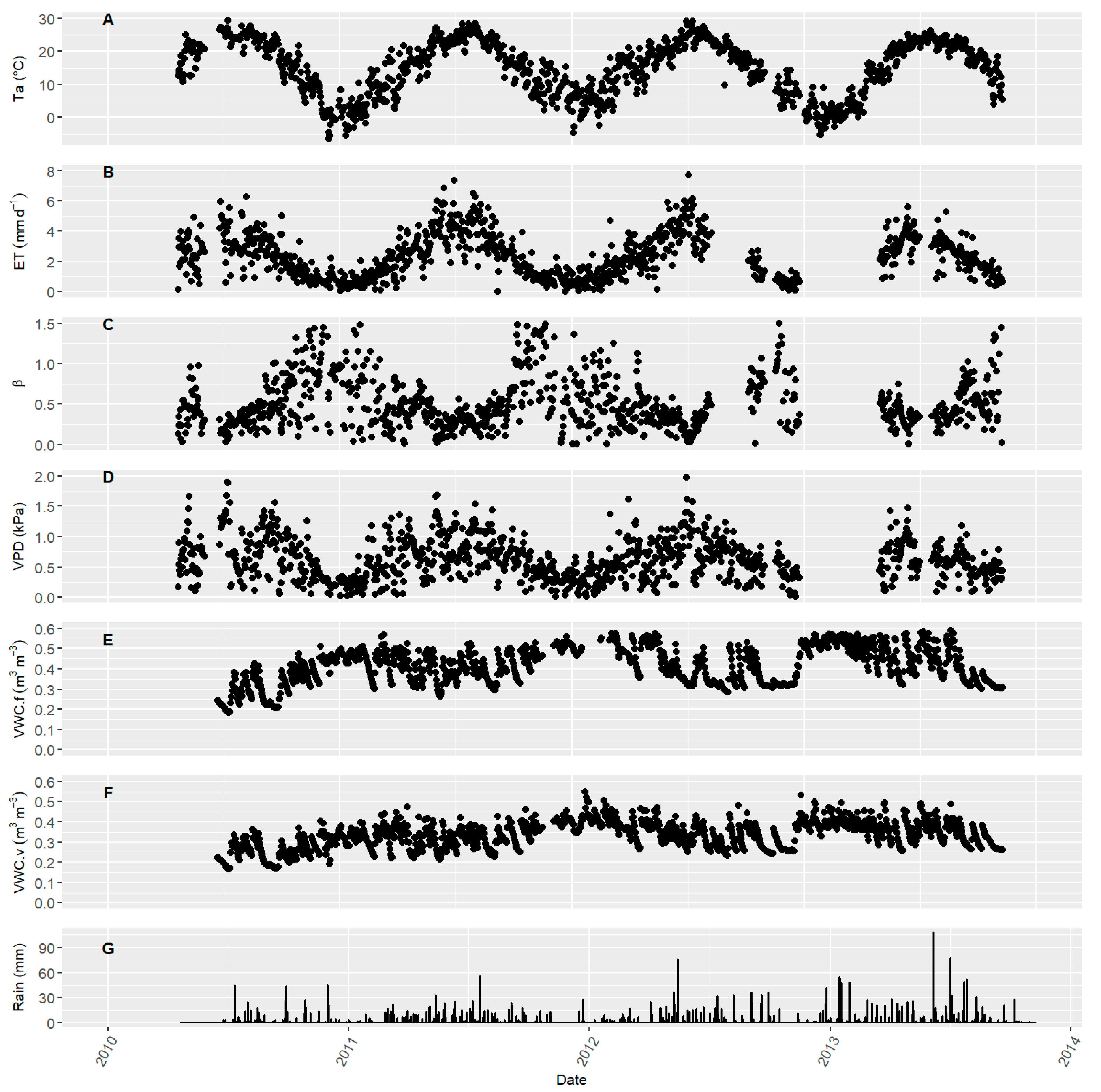
Daily ET, Ta, and VPD showed the typical seasonal pattern with high values during summer and low values during winter (Figure 1A,B,D). The VPD reached values of up to 1.90 kPa. Maximum ET in the growing season (i.e., May to October) ranged from 5.6 mm day−1 in 2013 to 7.7 mm day−1 in 2012. During the growing season median β was between 0.36 and 0.40, and in the off-season, it was between 0.47–0.84 (Figure 1C). The VWC in the surface 6 cm of soil under tall fescue ranged from 0.29 m3 m−3 in 2010 and 0.42 m3 m−3 in 2013, and under grapevines VWC was between 0.24–0.35 m3 m−3. The VWC pattern closely followed rainfall-events (Figure 1E–G). Mean annual ET was 752 ± 59 mm year−1. Note that the small annual ET in 2010 was related to the late onset of the study and a data gap from DOY 153–175 (Table 1, Figure 1B). Precipitation (P) was above ET in 2010 –2013 with a mean P-ET ratio of 1.21.
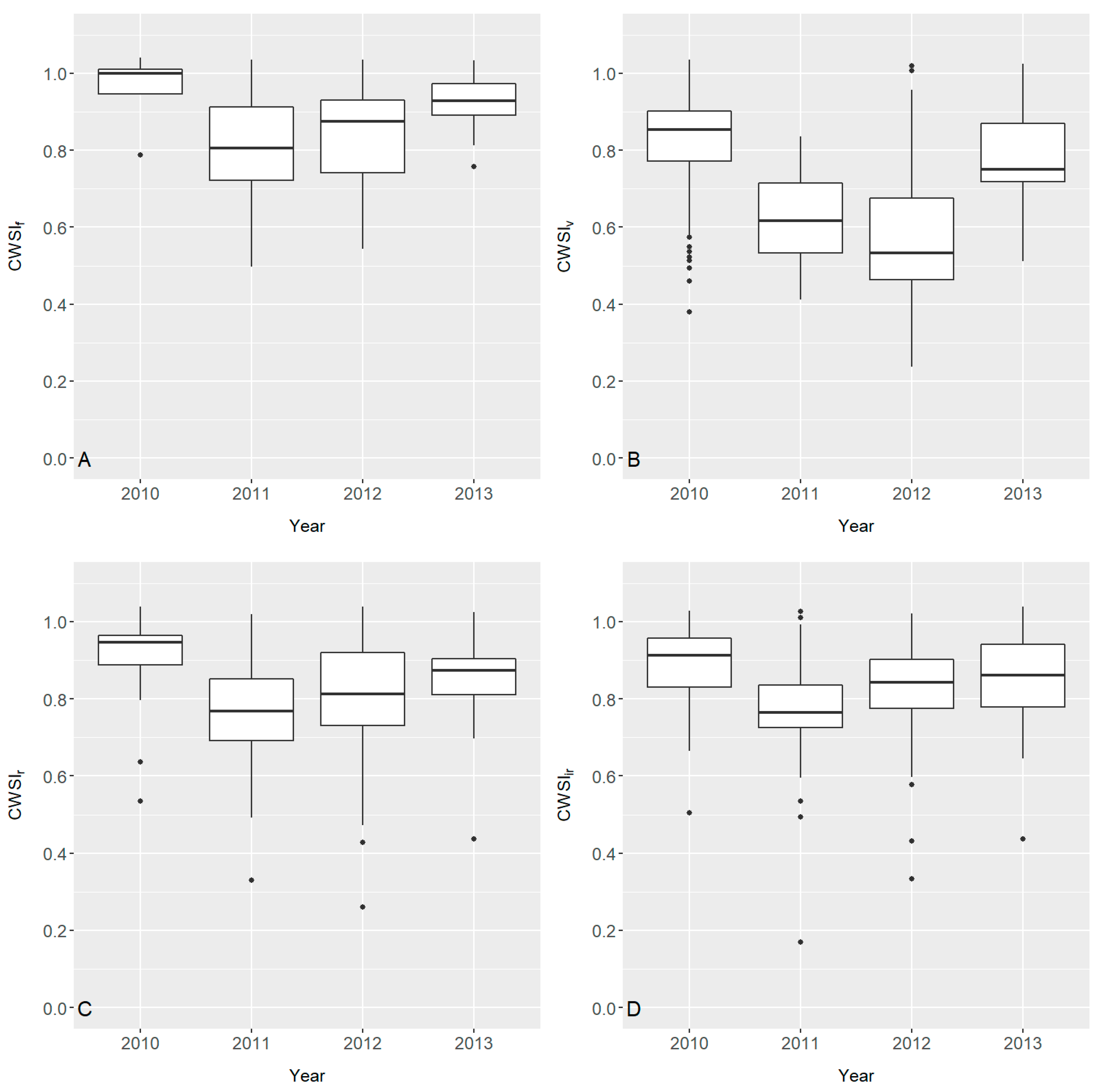
The dTmin values of fescue, grapevines, and measurements at 6.1 m above row and interrow was significantly related to VPD (p < 0.05), explaining 93–95% of the variation. The median CWSIf was lowest in 2011 with 0.81 and highest in 2010 with 1.0, and for CWSIv was lowest in 2010 with 0.53 and highest in 2013 with 0.85, respectively. The annual median CWSIir and CWSIr ranged between 0.76 and 0.91 and between 0.77 and 0.91, respectively. The CWSI was highly variable among years (Figure 2). There was a significantly negative linear relationship between ET and CWSIr (p < 0.05), i.e., with increasing CWSI the ET decreased. However, the relationship could only explain 15% of the variation.
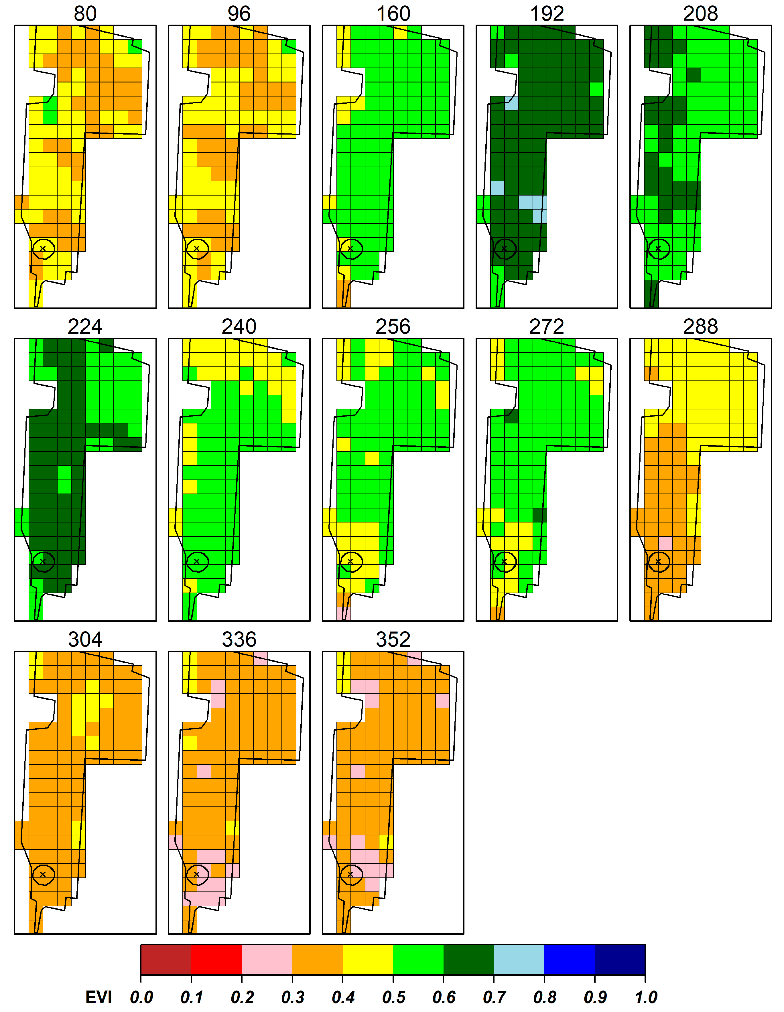
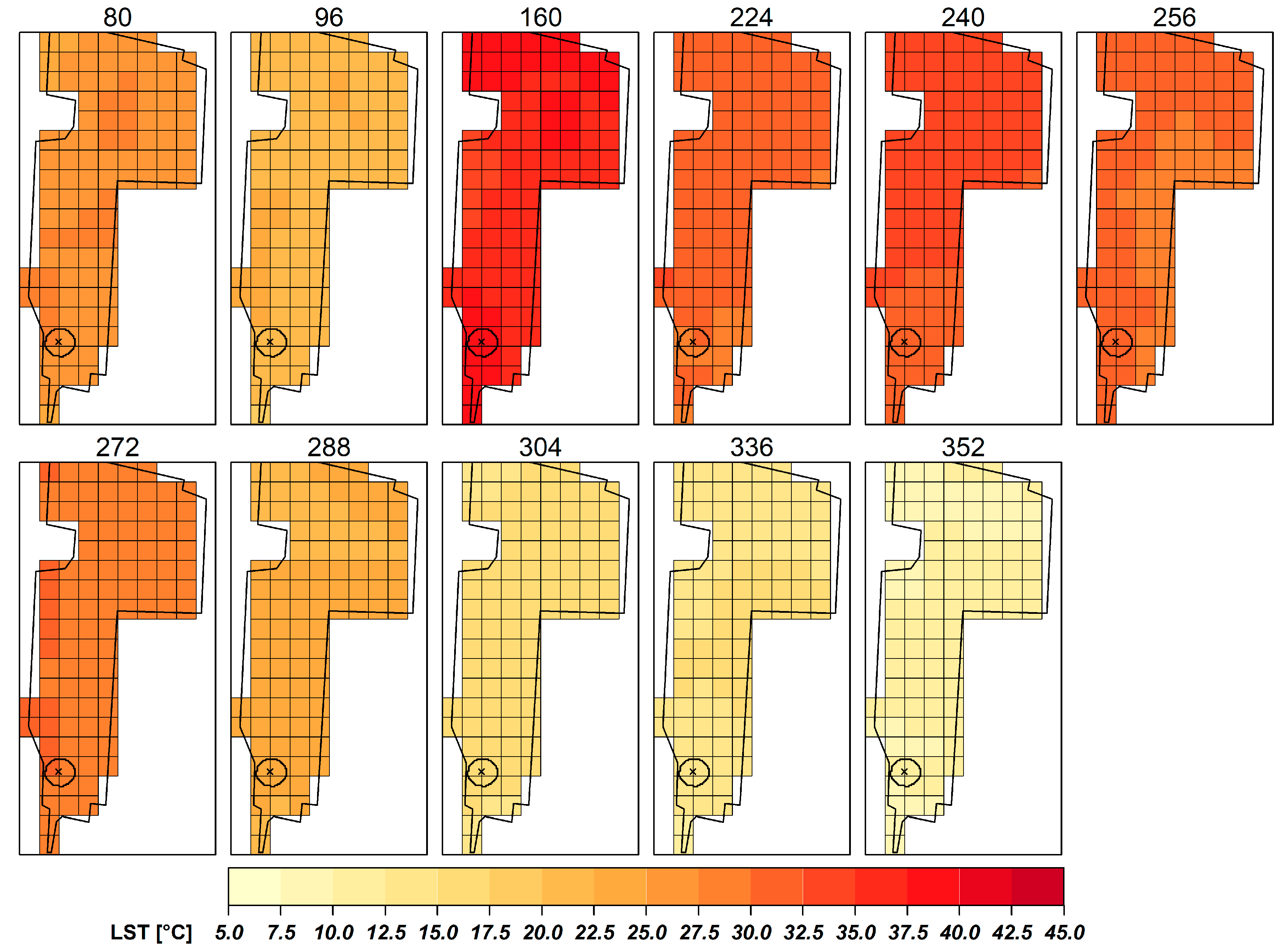
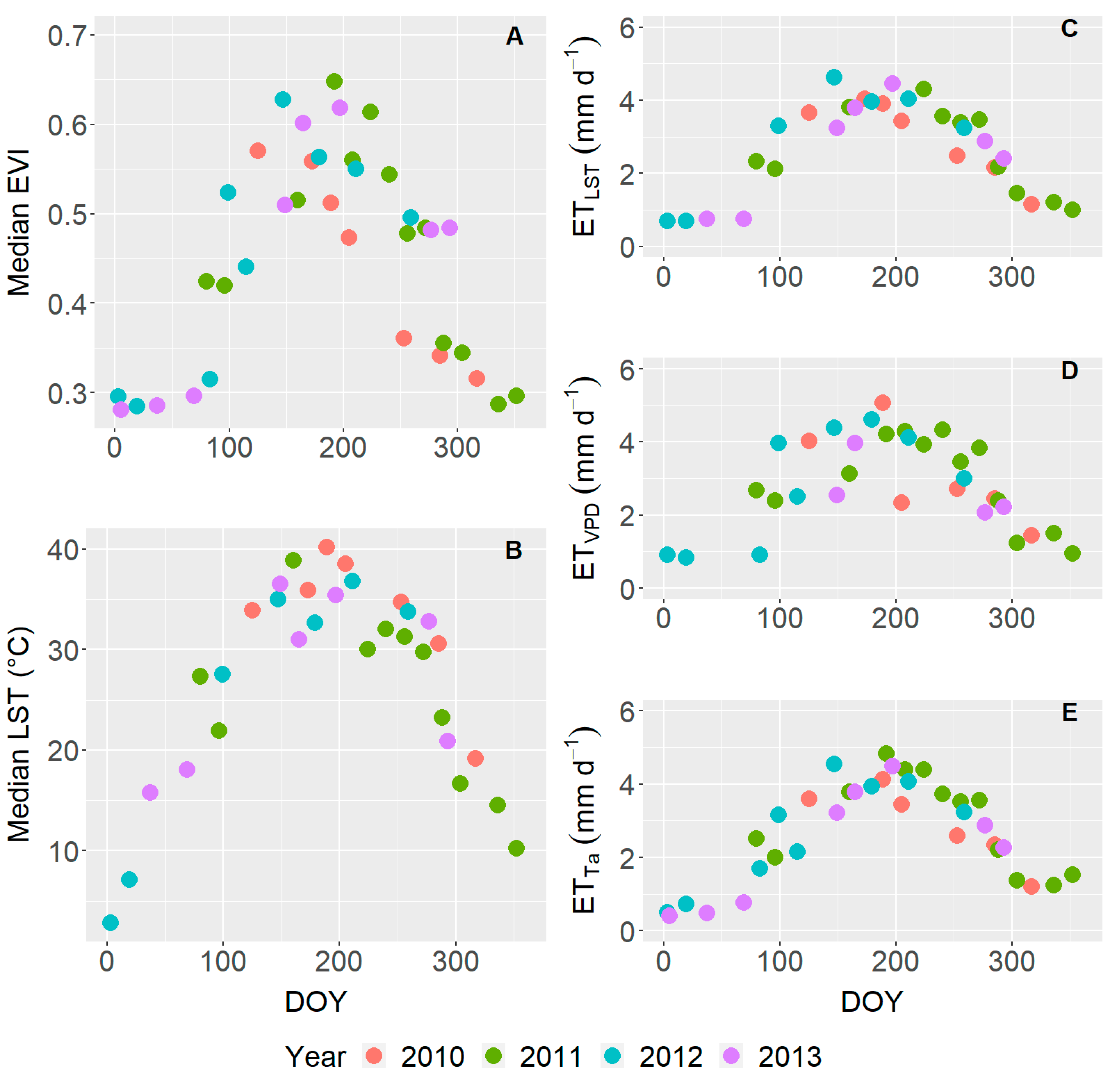
Vineyard median EVI ranged from 0.22–0.72 (Figure 3), with a mean within-vineyard range (calculated as the difference of maximum and minimum EVI) of 0.18. Median vineyard LST ranged from 16.0–40.1 °C from 2010 to 2013, with a mean range within the vineyard of 4.44 °C (Figure 4). Median EVI within the EC footprint followed a seasonal pattern and ranged from 0.28–0.65 (Figure 5A). Median LST within the EC footprint also followed a seasonal pattern and ranged from 0.8 to 42.6 °C (Figure 5B). The LST was significantly related to Tc at overpass time and lowest RMSE of 1.13 °C was measured with an IRT sensor at 6.1 m above the grapevine row (Table 2).
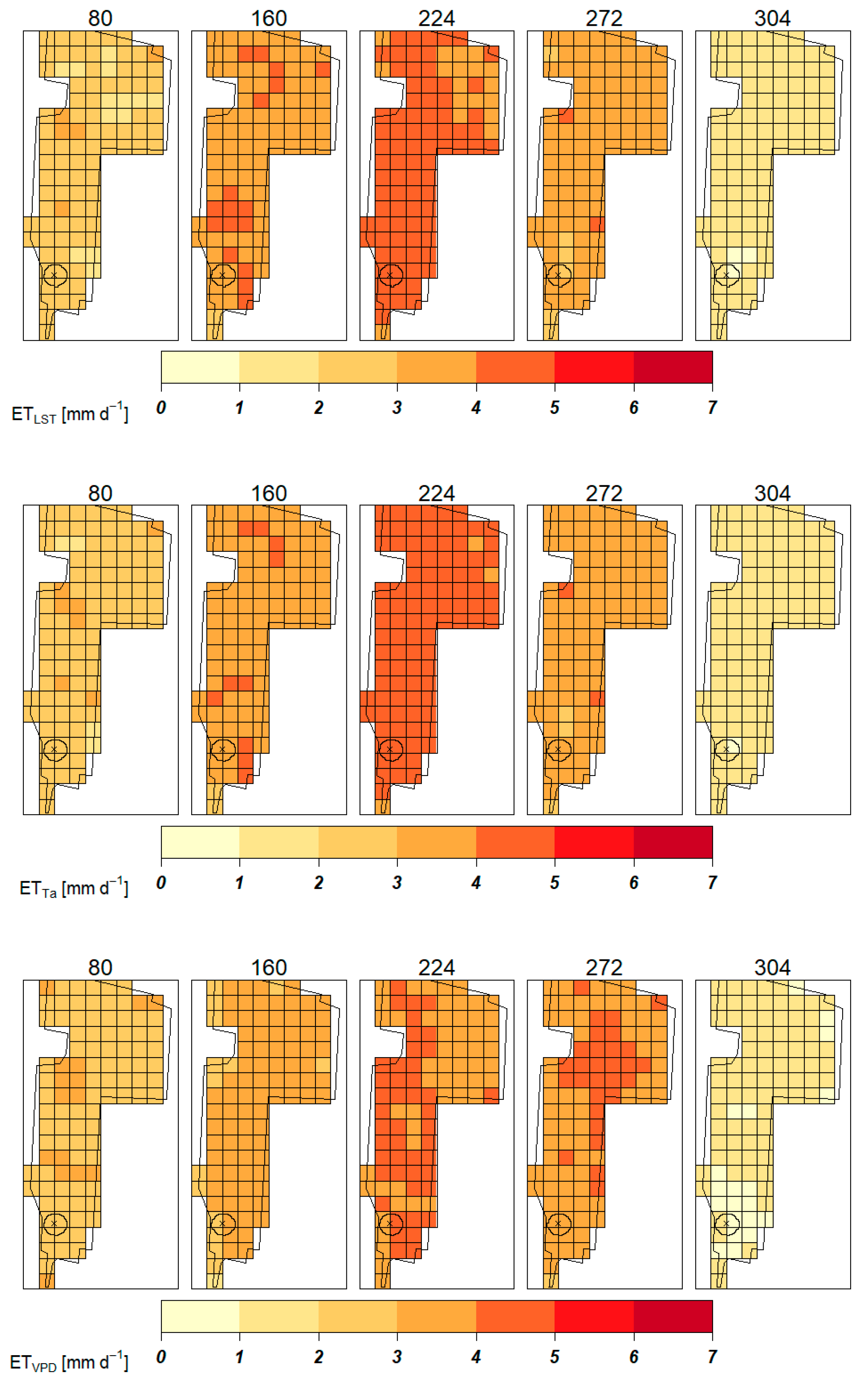
Footprint EVI and on-site Ta, LST, and VPD were used as independent variables to establish multiple linear regression models with ET as the dependent variable (Table 3). All models were significant at p < 0.05, explaining 75% to 84% of the variation. All parameters had a positive linear relationship to ET, i.e., with increasing EVI, Ta, LST or VPD, the daily ET increased and vice versa. A linear regression analysis between calculated ET and measured ET was significant at p < 0.05 and had a root mean square error (RMSE) of 0.52–0.62 mm (Table 3). Note that combining more independent variables did not improve the empirical models, so the more parsimonious models were chosen. While the overall EVI-LST model was significant, the LST parameter was only significant at p < 0.1, due to higher variation in the LST dataset. The derived coefficients were then used to calculate vineyard ET. Median daily vineyard ETTa, ETLST, and ETVPD ranged from 0.4–4.8, 0.7–4.6, and 0.8–5.1 mm day−1, respectively (Figure 5C–E). The mean within-vineyard ET range was 1.31, 1.67, and 1.48 mm for ETTa, ETLST, and ETVPD, respectively (Figure 6).
4. Discussion
In this study, ET was measured using an EC system in a NC vineyard. Similar daily ET values for interrrow areas had previously been measured with a micro-Bowen Ratio energy balance system (MBR) [24], showing that the estimated ET values were reasonable. The authors also showed that the interrow tall fescue increased ET compared to bare soil, and that the contribution of tall fescue to ET was higher in the off season than during the growing season [24]. Note that ET measured with the EC system was a shared signal of both, vines and tall fescue, as the EC footprint was greater than for the MBRs.
The Landsat 7 EVI and LST were as well based on the reflectance of both, vines and grass at a resolution of 30 × 30 m. The LST was best correlated with Tcr and Tcir (Table 2), probably owing to the higher IRT footprint measuring a combined signal of interrow, soil, and vines. Significant relationships with Landsat brightness temperature and IRT sensor measurements [42], and Landsat LST and soil temperature [43] had previously been reported. The ET values presented were specific to the local environment as well as vineyard management (as described by LST, EVI, and EC derived data), and any upscaling approaches for other systems may need additional adjustments.
The VWC at 6 cm soil depth was mostly above the wilting point of 0.27 m3 m−3 during the study period [44], especially under tall fescue, which would indicate no severe water-stress soil conditions. Yet, CWSI values were relatively high, an indicator that water-stress occurred, at least during high-radiation time periods during midday. In a Mediterranean vineyard CWSI values from 0.45−0.65 were reported, which was lower than in this study [12]. The authors also found a positive relation between yield parameters and CWSI, the higher the CWSI the higher the berry weight. Assuming a similar yield response, mid-season CWSI would indicate water stress levels that would benefit yield but would be too high at the onset of the growing season, when water stress is not beneficial. Yet, yield also depends on berry and cluster number, and other factors such as trimming can further influence yield. Thus, further analysis with a larger dataset including yield data would be needed to confirm this relationship for our study. The linear relationship between ET and CWSIv would indicate the effect of evaporative cooling on Tc (Equation 1), and similar relationships have previously been reported for other agro-ecosystems [45]. Yet, CWSI was a weak predictor of ET compared to EVI, Ta, LST, or VPD in this study. The footprint of EC derived ET was greater than IRT-measured Tc. In addition, the CWSI was calculated for midday time periods on days with high net radiation, that is periods of maximum water stress. This may explain the weak relationship with EC-measured daily ET values.
In a previous study, EVI and Ta were used as substitutes for kc and ET0 to estimate ET from riparian vegetation [14]. In this study, ETTa showed good agreement with measured ET, demonstrating that EVI and Ta can be used to estimate ET. However, the best ET estimates were achieved with VPD as the independent variable. [14] found a sigmoidal relationship with Ta and an exponential relationship with EVI. This was not the case in this study, where a linear relationship was used. There was no upper asymptote in the ET-Ta relationship, i.e., there was still an ET response even at maximum Ta. However, this may not be the case for exceptionally dry and hot years, where the model presented may overestimate ET.
Estimating ETTa requires only a point measurement of Ta and EVI maps. Yet, higher accuracy (i.e., lowest RMSE) was achieved with VPD as the independent variable, however, this would require two measurements, Ta and rH or water vapor density. ETTa and ETVPD estimation assumed that Ta and rH did not substantially change within the vineyard. However, even on smaller scales (field-level) we found substantial variation in LST, and it may be recommended to use satellite-derived LST for ET upscaling [3,4]. The drawback using Landsat VI and LST products was that Landsat had a 16-day overpass-period, and cloud cover could impact the image quality. Data fusion approaches or other interpolation methods may then be needed to generate datasets in shorter time periods [3]. Despite these caveats, it was possible to accurately upscale ET for the whole vineyard with these parsimonious models.
Author Contributions
Conceptualization, G.G., J.H. and T.S.; methodology, A.H., C.D., J.H. and T.S.; software, A.H. and C.D.; validation, G.G., J.H. and T.S.; formal analysis, C.D.; investigation, A.H., J.H. and T.S.; resources, G.G., J.H., J.H. and T.S.; data curation, A.H. and C.D.; writing—original draft preparation, C.D.; writing—review and editing, A.H., C.D., G.G., J.H., J.H. and T.S.; visualization, C.D.; supervision, J.H. and T.S.; project administration, A.H., G.G.,J.H., J.H. and T.S; funding acquisition, J.H., J.H. and T.S.
Funding
This research was supported in part by an appointment to the Agricultural Research Service (ARS) Research Participation Program administered by the Oak Ridge Institute for Science and Education (ORISE) through an interagency agreement between the U.S. Department of Energy (DOE) and the U.S. Department of Agriculture (USDA). ORISE is managed by ORAU under DOE contract number DE-AC05-06OR23100. This study was supported by the Binational Agricultural Research and Development Fund (BARD US-4262-09). All opinions expressed in this paper are the author’s and do not necessarily reflect the policies and views of USDA, ARS, DOE, or ORAU/ORISE.
Acknowledgments
The authors gratefully acknowledge Shelton Vineyards for providing the study site and assisting with maintenance. We would like to thank the anonymous reviewers for their comments which greatly improved this manuscript.
Conflicts of Interest
The authors declare no conflicts of interest.
References
- Williams, L.E.; Grimes, D.; Phene, C. The effects of applied water at various fractions of measured evapotranspiration on reproductive growth and water productivity of Thompson Seedless grapevines. Irrig. Sci. 2010, 28, 233–243. [Google Scholar] [CrossRef]
- Carrasco-Benavides, M.; Ortega-Farías, S.; Lagos, L.; Kleissl, J.; Morales-Salinas, L.; Kilic, A. Parameterization of the Satellite-Based Model (METRIC) for the Estimation of Instantaneous Surface Energy Balance Components over a Drip-Irrigated Vineyard. Remote Sens. 2014, 6, 11342–11371. [Google Scholar] [CrossRef]
- Semmens, K.A.; Anderson, M.C.; Kustas, W.P.; Gao, F.; Alfieri, J.G.; McKee, L.; Prueger, J.H.; Hain, C.R.; Cammalleri, C.; Yang, Y.; et al. Monitoring daily evapotranspiration over two California vineyards using Landsat 8 in a multi-sensor data fusion approach. Remote Sens. Environ. 2016, 185, 155–170. [Google Scholar] [CrossRef]
- Galleguillos, M.; Jacob, F.; Prévot, L.; French, A.; Lagacherie, P. Comparison of two temperature differencing methods to estimate daily evapotranspiration over a Mediterranean vineyard watershed from ASTER data. Remote Sens. Environ. 2011, 115, 1326–1340. [Google Scholar] [CrossRef]
- Burba, G. Eddy Covariance Method for Scientific, Industrial, Agricultural and Regulatory Applications: A Field Book on Measuring Ecosystem Gas Exchange and Areal Emission Rates; LI-COR Biosciences: Lincoln, NE, USA, 2013; 331p. [Google Scholar]
- Idso, S.; Jackson, R.; Pinter, P.; Reginato, R.; Hatfield, J. Normalizing the stress-degree-day parameter for environmental variability. Agric. Meteorol. 1981, 24, 45–55. [Google Scholar] [CrossRef]
- Jackson, R.; Idso, S.; Reginato, R.; Pinter, P. Canopy temperature as a crop water stress indicator. Water Resour. Res. 1981, 17, 1133–1138. [Google Scholar] [CrossRef]
- Gardner, B.; Nielsen, D.; Shock, C. Infrared thermometry and the crop water stress index. II. Sampling procedures and interpretation. J. Prod. Agric. 1992, 5, 466–475. [Google Scholar] [CrossRef]
- Payero, J.; Irmak, S. Variable upper and lower crop water stress index baselines for corn and soybean. Irrig. Sci. 2006, 25, 21–32. [Google Scholar] [CrossRef]
- Bellvert, J.; Zarco-Tejada, P.J.; Girona, J.; Fereres, E. Mapping crop water stress index in a ‘Pinot-noir’ vineyard: Comparing ground measurements with thermal remote sensing imagery from an unmanned aerial vehicle. Precis. Agric. 2014, 15, 361–376. [Google Scholar] [CrossRef]
- Bellvert, J.; Zarco-Tejada, P.J.; Marsal, J.; Girona, J.; González-Dugo, V.; Fereres, E. Vineyard irrigation scheduling based on airborne thermal imagery and water potential thresholds. Aust. J. Grape Wine Res. 2016, 22, 307–315. [Google Scholar] [CrossRef]
- Santesteban, L.G.; Di Gennaro, S.F.; Herrero-Langreo, A.; Miranda, C.; Royo, J.B.; Matese, A. High-resolution UAV-based thermal imaging to estimate the instantaneous and seasonal variability of plant water status within a vineyard. Agric. Water Manag. 2017, 183, 49–59. [Google Scholar] [CrossRef]
- Poblete-Echeverría, C.; Espinace, D.; Sepúlveda-Reyes, D.; Zúñiga, M.; Sanchez, M. Analysis of crop water stress index (CWSI) for estimating stem water potential in grapevines: Comparison between natural reference and baseline approaches. Acta Hortic. 2017, 1150, 189–194. [Google Scholar] [CrossRef]
- Anderson, M.C.; Allen, R.G.; Morse, A.; Kustas, W.P. Use of Landsat thermal imagery in monitoring evapotranspiration and managing water resources. Remote Sens. Environ. 2012, 122, 50–65. [Google Scholar] [CrossRef]
- Bastiaanssen, W.G.M.; Menenti, M.; Feddes, R.A.; Holtslag, A.A.M. A remote sensing surface energy balance algorithm for land (SEBAL). 1. Formulation. J. Hydrol. 1998, 212–213, 198–212. [Google Scholar] [CrossRef]
- Allen, R.G.; Tasumi, M.; Trezza, R. Satellite-Based Energy Balance for Mapping Evapotranspiration with Internalized Calibration (METRIC)-Model. J. Irrig. Drain. Eng. 2007, 133, 380–394. [Google Scholar] [CrossRef]
- Roerink, G.J.; Su, Z.; Menenti, M. S-SEBI: A simple remote sensing algorithm to estimate the surface energy balance. Phys. Chem. Earth Part B Hydrol. Oceans Atmos. 2000, 25, 147–157. [Google Scholar] [CrossRef]
- Cammalleri, C.; Anderson, M.C.; Gao, F.; Hain, C.R.; Kustas, W.P. A data fusion approach for mapping daily evapotranspiration at field scale. Water Resour. Res. 2013, 49, 4672–4686. [Google Scholar] [CrossRef]
- Zhang, K.; Kimball, J.S.; Running, S.W. A review of remote sensing based actual evapotranspiration estimation. Wiley Interdiscip. Rev. Water 2016, 3, 834–853. [Google Scholar] [CrossRef]
- Vivoni, E.R.; Moreno, H.A.; Mascaro, G.; Rodriguez, J.C.; Watts, C.J.; Garatuza-Payan, J.; Scott, R.L. Observed relation between evapotranspiration and soil moisture in the North American monsoon region. Geophys. Res. Lett. 2008, 35, L22403. [Google Scholar] [CrossRef]
- Allen, R.G.; Pereira, L.S.; Raes, D.; Smith, M. Crop Evapotranspiration-Guidelines for Computing Crop Water Requirements—FAO Irrigation and Drainage Paper 56; FAO: Rome, Italy, 1998; p. 174. [Google Scholar]
- Choudhury, B.J.; Ahmed, N.U.; Idso, S.B.; Reginato, R.J.; Daughtry, C.S.T. Relations between evaporation coefficients and vegetation indices studied by model simulations. Remote Sens. Environ. 1994, 50, 1–17. [Google Scholar] [CrossRef]
- Nagler, P.L.; Scott, R.L.; Westenburg, C.; Cleverly, J.R.; Glenn, E.P.; Huete, A.R. Evapotranspiration on western U.S. rivers estimated using the Enhanced Vegetation Index from MODIS and data from eddy covariance and Bowen ratio flux towers. Remote Sens. Environ. 2005, 97, 337–351. [Google Scholar] [CrossRef]
- Holland, S.; Heitman, J.L.; Howard, A.; Sauer, T.J.; Giese, W.; Ben-Gal, A.; Agam, N.; Kool, D.; Havlin, J. Micro-Bowen ratio system for measuring evapotranspiration in a vineyard interrow. Agric. For. Meteorol. 2013, 177, 93–100. [Google Scholar] [CrossRef]
- Tanner, C.B.; Thurtell, G.W. Anemoclinometer Measurements of Reynolds Stress and Heat Transport in the Atmospheric Surface Layer; Wisconsin University-Madison, Department of Soil Science: Madison, WI, USA, 1969; pp. 1–10. [Google Scholar]
- Webb, E.; Pearman, G.; Leuning, R. Correction of flux measurements for density effects due to heat and water vapour transfer. Q. J. R. Meteorol. Soc. 1980, 106, 85–100. [Google Scholar] [CrossRef]
- Hernandez-Ramirez, G.; Hatfield, J.L.; Parkin, T.B.; Sauer, T.J.; Prueger, J.H. Carbon dioxide fluxes in corn–soybean rotation in the midwestern US: Inter-and intra-annual variations, and biophysical controls. Agric. For. Meteorol. 2011, 151, 1831–1842. [Google Scholar] [CrossRef]
- Baker, J.; Griffis, T. Examining strategies to improve the carbon balance of corn/soybean agriculture using eddy covariance and mass balance techniques. Agric. For. Meteorol. 2005, 128, 163–177. [Google Scholar] [CrossRef]
- Hernandez-Ramirez, G.; Hatfield, J.L.; Prueger, J.H.; Sauer, T.J. Energy balance and turbulent flux partitioning in a corn–soybean rotation in the Midwestern US. Theor. Appl. Climatol. 2010, 100, 79–92. [Google Scholar] [CrossRef]
- Schmidt, M.; Reichenau, T.G.; Fiener, P.; Schneider, K. The carbon budget of a winter wheat field: An eddy covariance analysis of seasonal and inter-annual variability. Agric. For. Meteorol. 2012, 165, 114–126. [Google Scholar] [CrossRef]
- Allen, R.G.; Pruitt, W.O. FAO-24 reference evapotranspiration factors. J. Irrig. Drain. Eng. 1991, 117, 758–773. [Google Scholar] [CrossRef]
- Dold, C.; Büyükcangaz, H.; Rondinelli, W.; Prueger, J.; Sauer, T.; Hatfield, J. Long-term carbon uptake of agro-ecosystems in the Midwest. Agric. For. Meteorol. 2017, 232, 128–140. [Google Scholar] [CrossRef]
- Jackson, R.D.; Kustas, W.P.; Choudhury, B.J. A reexamination of the crop water stress index. Irrig. Sci. 1988, 9, 309–317. [Google Scholar] [CrossRef]
- Lowe, P.R. An Approximating Polynomial for the Computation of Saturation Vapor Pressure. J. Appl. Meteorol. 1977, 16, 100–103. [Google Scholar] [CrossRef]
- Ham, J.M. Useful equations and tables in micrometeorology. Micrometeorol. Agric. Syst. 2005, 47, 533–560. [Google Scholar]
- Thom, A.S.; Oliver, H.R. On Penman’s equation for estimating regional evaporation. Q. J. R. Meteorol. Soc. 1977, 103, 345–357. [Google Scholar] [CrossRef]
- Sauer, T.J.; Horton, R. Soil Heat Flux. Micrometeorol. Agric. Syst. 2005, 47, 131–154. [Google Scholar]
- Masek, J.G.; Vermote, E.F.; Saleous, N.E.; Wolfe, R.; Hall, F.G.; Huemmrich, K.F.; Feng, G.; Kutler, J.; Teng-Kui, L. A Landsat surface reflectance dataset for North America, 1990–2000. IEEE Geosci. Remote Sens. Lett. 2006, 3, 68–72. [Google Scholar] [CrossRef]
- Cook, M.; Schott, J.R.; Mandel, J.; Raqueno, N. Development of an Operational Calibration Methodology for the Landsat Thermal Data Archive and Initial Testing of the Atmospheric Compensation Component of a Land Surface Temperature (LST) Product from the Archive. Remote Sens. 2014, 6, 11244–11266. [Google Scholar] [CrossRef]
- United States Geological Survey (USGS). Landsat Level-2 Provisional Surface Temperature Science Product 2019. Available online: https://www.usgs.gov/land-resources/nli/landsat/landsat-provisional-surface-temperature (accessed on 21 March 2019).
- R Core Team. R: A Language and Environment for Statistical Computing; R Foundation for Statistical Computing: Vienna, Austria, 2014. [Google Scholar]
- Li, F.; Jackson, T.J.; Kustas, W.P.; Schmugge, T.J.; French, A.N.; Cosh, M.H.; Bindlish, R. Deriving land surface temperature from Landsat 5 and 7 during SMEX02/SMACEX. Remote Sens. Environ. 2004, 92, 521–534. [Google Scholar] [CrossRef]
- Veysi, S.; Naseri, A.A.; Hamzeh, S.; Bartholomeus, H. A satellite based crop water stress index for irrigation scheduling in sugarcane fields. Agric. Water Manag. 2017, 189, 70–86. [Google Scholar] [CrossRef]
- Holland, S.; Howard, A.; Heitman, J.L.; Sauer, T.J.; Giese, W.; Sutton, T.B.; Agam, N.; Ben-Gal, A.; Havlin, J. Implications of Tall Fescue for Inter-Row Water Dynamics in a Vineyard. Agron. J. 2014, 106, 1267–1274. [Google Scholar] [CrossRef]
- Dold, C.; Hatfield, J.L.; Prueger, J.; Sauer, T.; Büyükcangaz, H.; Rondinelli, W. Long-Term Application of the Crop Water Stress Index in Midwest Agro-Ecosystems. Agron. J. 2017, 109. [Google Scholar] [CrossRef]
Figure 1.
Daily air temperature (Ta) (A), evapotranspiration (ET) (B), and Bowen Ratio (β) (C), vapor pressure deficit (VPD) (D), volumetric soil water content in 6 cm soil depth under tall fescue (VWC.f) (E), and grapevines (VWC.v) (F), and daily precipitation (G) from 2010 to 2013 in a NC vineyard.

Figure 2.
Daily Crop Water Stress Index (CWSI) for tall fescue (A), grapevines (B), above the vine row (C) and interrow (D) in 6.1 m during the months of May to October, from 2010–2013.
Figure 2.
Daily Crop Water Stress Index (CWSI) for tall fescue (A), grapevines (B), above the vine row (C) and interrow (D) in 6.1 m during the months of May to October, from 2010–2013.

Figure 3.
Enhanced Vegetation Index (EVI) for the whole vineyard in 2011 from 13 Landsat 7 images between DOY 80 and DOY 352. The cross shows the position of the EC system with the 80% footprint area.
Figure 3.
Enhanced Vegetation Index (EVI) for the whole vineyard in 2011 from 13 Landsat 7 images between DOY 80 and DOY 352. The cross shows the position of the EC system with the 80% footprint area.

Figure 4.
Land surface temperature (LST) for the whole vineyard in 2011 from eleven Landsat 7 images between DOY 80 and DOY 352. The cross shows the position of the EC system with the 80% footprint area.
Figure 4.
Land surface temperature (LST) for the whole vineyard in 2011 from eleven Landsat 7 images between DOY 80 and DOY 352. The cross shows the position of the EC system with the 80% footprint area.

Figure 5.
Median EVI (A) and LST (B) within the EC footprint derived from Landsat imagery, and modeled daily vineyard ET as calculated with EVI and LST (C), VPD (D), and Ta (E), respectively.
Figure 5.
Median EVI (A) and LST (B) within the EC footprint derived from Landsat imagery, and modeled daily vineyard ET as calculated with EVI and LST (C), VPD (D), and Ta (E), respectively.

Figure 6.
Modeled daily ET for the whole vineyard in 2011 from DOY 80−304 as calculated from EVI in conjunction with LST (ETLST), Ta (ETTa), and VPD (ETVPD), respectively. The cross shows the position of the EC system with the 80% footprint area around the EC station.
Figure 6.
Modeled daily ET for the whole vineyard in 2011 from DOY 80−304 as calculated from EVI in conjunction with LST (ETLST), Ta (ETTa), and VPD (ETVPD), respectively. The cross shows the position of the EC system with the 80% footprint area around the EC station.


Table 1.
Annual evapotranspiration (ET) from 2010–2013.
| Year | ET (mm year−1) |
|---|---|
| 2010 | 579 |
| 2011 | 837 |
| 2012 | 807 |
| 2013 | 784 |
| Mean | 752 ± 59 |
Table 2.
The RMSE (°C), and R2 of linear regression models with Tc (°C) measured with IRT sensors at time of satellite overpass as independent variable, and LST (°C) as dependent variable.
Table 2.
The RMSE (°C), and R2 of linear regression models with Tc (°C) measured with IRT sensors at time of satellite overpass as independent variable, and LST (°C) as dependent variable.
| Tc | R2 | RMSE (°C) |
|---|---|---|
| Tcf | 0.99 | 2.18 |
| Tcv | 1.00 | 1.68 |
| Tcr | 1.00 | 1.13 |
| Tcir | 1.00 | 1.49 |
IRT = infrared temperature; RMSE = root mean squared error, R2 = coefficient of determination; LST = Land surface temperature, Tc = canopy temperature.
Table 3.
Coefficients of a multiple linear regression analysis with EVI and Ta, VPD, or LST as independent and ET as dependent variable. The RMSE refers to ET measured with the EC station versus modeled ET within the 80% footprint area.
Table 3.
Coefficients of a multiple linear regression analysis with EVI and Ta, VPD, or LST as independent and ET as dependent variable. The RMSE refers to ET measured with the EC station versus modeled ET within the 80% footprint area.
| Model | Coefficients | Mean | SE | p | Adj. R2 | dF | Variable range | Adj. R2 Measured vs. Modeled ET | RMSE Measured vs. Modeled ET |
|---|---|---|---|---|---|---|---|---|---|
| ETTa | Intercept | −1.629 | 0.592 | <0.05 | 0.76 | 28 | 0.77 | 0.60 | |
| EVI | 7.181 | 1.821 | <0.001 | 0.28–0.65 | |||||
| Ta (°C) | 0.069 | 0.025 | <0.01 | −4.55–29.32 | |||||
| ETVPD | Intercept | −2.131 | 0.457 | <0.001 | 0.84 | 28 | 0.84 | 0.52 | |
| EVI | 7.866 | 1.159 | <0.001 | 0.28–0.65 | |||||
| VPD (kPa) | 1.645 | 0.332 | <0.001 | 0.23–1.89 | |||||
| ETLST | Intercept | −2.438 | 0.631 | <0.001 | 0.75 | 24 | 0.76 | 0.62 | |
| EVI | 8.877 | 2.017 | <0.001 | 0.28–0.63 | |||||
| LST (°C) | 0.042 | 0.021 | <0.1 | 2.81–40.15 |
Adj. R2 = adjusted coefficient of determination, dF = degrees of freedom, EVI = Enhanced Vegetation Index, LST = Land surface temperature, RMSE = root mean squared error, Ta = air temperature, SE= standard error, p = significance level, VPD = vapor pressure deficit.
© 2019 by the authors. Licensee MDPI, Basel, Switzerland. This article is an open access article distributed under the terms and conditions of the Creative Commons Attribution (CC BY) license (http://creativecommons.org/licenses/by/4.0/).
Share and Cite
MDPI and ACS Style
Dold, C.; Heitman, J.; Giese, G.; Howard, A.; Havlin, J.; Sauer, T. Upscaling Evapotranspiration with Parsimonious Models in a North Carolina Vineyard. Agronomy 2019, 9, 152. https://0-doi-org.brum.beds.ac.uk/10.3390/agronomy9030152
AMA Style
Dold C, Heitman J, Giese G, Howard A, Havlin J, Sauer T. Upscaling Evapotranspiration with Parsimonious Models in a North Carolina Vineyard. Agronomy. 2019; 9(3):152. https://0-doi-org.brum.beds.ac.uk/10.3390/agronomy9030152
Chicago/Turabian StyleDold, Christian, Joshua Heitman, Gill Giese, Adam Howard, John Havlin, and Tom Sauer. 2019. "Upscaling Evapotranspiration with Parsimonious Models in a North Carolina Vineyard" Agronomy 9, no. 3: 152. https://0-doi-org.brum.beds.ac.uk/10.3390/agronomy9030152
Note that from the first issue of 2016, this journal uses article numbers instead of page numbers. See further details here.