Multi-Year N and P Removal of a 10-Year-Old Surface Flow Constructed Wetland Treating Agricultural Drainage Waters

Abstract

Surface flow constructed wetlands (SFCWs) can be effectively used to treat agricultural drainage waters, reducing N and P surface water pollution. In the Venice Lagoon drainage basin (northeastern Italy), an SFCW was monitored during 2007–2013 to assess its performance in reducing water, N, and P loads more than 10 years after its creation. Nitrogen concentrations showed peaks during winter due to intense leaching from surrounding fields. Phosphorus concentrations were higher after prolonged periods with no discharge, likely due to mobilization of P of the decomposing litter inside the basin. Over the entire period, N removal efficiency was 83% for NO₃–N and 79% for total N; P removal efficiency was 48% for PO₄–P and 67% for total P. Values were higher than in several other studies, likely due to the fluctuating hydroperiod that produced discontinuous and reduced outflows. Nitrogen outlet concentrations were reduced by the SFCW, and N removal ratios decreased with increasing hydraulic loading, while no strong correlations were found in the case of P. The SFCW was shown to be an effective long-term strategy to increase water storage and reduce N and P loads in the Venice Lagoon drainage basin.

1. Introduction

Surface flow constructed wetlands (SFCWs) are nature-based solutions, created to mimic natural systems [1], where plants (usually macrophytes) grow partly submerged in water, with the roots in the soil. Surface flow constructed wetlands are commonly used for the treatment of various type of wastewaters, ranging from urban, to the industrial and agricultural sectors [2], and for the provision of multiple ecosystem services [3]. In agricultural ecosystems, SFCWs are considered cost-effective in reducing nonpoint-source pollution, especially when treating agricultural surface waters that are rich in nutrients [4,5,6], especially nitrogen (N) and phosphorus (P) [7]. They perform particularly well in reducing nitrogen loads through nitrification-denitrification processes and plant uptake [8,9,10], whereas phosphorus removal largely depends on a combination of sedimentation, adsorption-desorption, complexation, and precipitation phenomena [6,11].

Despite several studies reporting that SFCWs can manage varying amounts of agricultural pollutants, N and P removals can range considerably, depending on input loads, wetland/catchment ratio, and site-specific pedoclimatic and meteorological conditions [6,12,13]. Vymazal [13], surveying the literature on full-scale constructed wetlands (CWs), found a variability of several orders of magnitude in N removal (from 11 to 13026 kg N ha⁻¹ per year). Similarly, Fisher and Acreman [14], reviewing the performances of N and P removal of riparian, floodplain, and marsh wetlands in different regions of the world, reported great variability in nutrient loading reduction (from 1% to 100% for N, and from 5% to 100% for P). However, the authors stressed that little evidence is available on the long-term P removal performances, as many studies were carried out for no more than two years. Short- and long-term SFCWs performance is debated: Reddy and DeBusk [15] and Borin and Tocchetto [16] suggested that in the initial phases, plants may play a greater role in determining N-removal performances, due to relatively rapid N uptake. Mitsch et al. [17] noted that P removal could decline in the long-term, possibly as a result of the saturation of storages in the sorptive matrix. However, another recent review [12] highlighted that CWs performance in removing total N and total P was mainly correlated with hydraulic loading rates, inlet concentrations, and climate zone indicators or average air temperature. The authors reported that most of the studies were conducted during the years following wetland creation or restoration (median of three years), thus questioning whether changes in wetland performances may occur depending on the operation time.

Considering the variability of wetland dynamics of different climatic areas, the annual fluctuations of wetland performances, the unforeseen effects of the aging of the wetland ecosystem, and the limited number of long-term experiments, it is pivotal to provide scientific evidence on water treatment performance of constructed wetlands in advanced stage, especially in areas where this technology has not previously been tested.

In this context, the Venice Lagoon drainage basin (in the northeastern part of the low-lying Padano-Veneta Valley in Italy) offers a suitable location to study the environmental benefits provided by SFCWs. Increasing concerns have been raised in the last decades about N and P surface water pollution of the Venice Lagoon [18,19,20], and the European Directives [21,22] stressed the need to reduce water and nutrient losses from agricultural fields to preserve the ecological status of European river basins [23].

The aim of this study was to assess the multi-year performance of an SFCW in removing N and P from agricultural drainage waters in a low-lying intensively cultivated area of northeastern Italy. The paper presents an overview of seven years of water, N, and P monitoring, in terms of nutrient concentrations, mass loads, and analysis of the main drivers determining the performances. The period analyzed in this study started 10 years after the wetland excavation.

2. Materials and Methods

2.1. Site Description

The SFCW is located at the experimental farm “L. Toniolo” of the University of Padova, in Legnaro, Padova (45°20′53″N, 11°57′11″, 6 m a.s.l.). The site is part of the Venice drainage watershed, in the northeastern low-lying Padano-Veneta Valley. The climate zone is part of the Cfa class (warm temperate climate with hot summers) in the Köppen classification [24].

A meteorological station of the Veneto regional agency for the environmental protection (ARPAV) is located at about 200 m from the SFCW. The station collects daily rainfall, temperature, and solar radiation data. Average annual rainfall is about 850 mm, with most falling in autumn and spring. Annual mean temperature is 13.5 °C, annual average minimum temperature is 8.7 °C, and annual average maximum is 18.6 °C. The month with the lowest average minimum temperature is January (−0.15 °C), while the month with the highest average maximum is July (29.5 °C). Evapotranspiration (ET₀) averages 995 mm y⁻¹, exceeding rainfall from April to September, especially during summer (June to August).

Soil of the experimental site is classified as Fluvi-Calcaric Cambisol (CMcf) [25], loam, or silty loam. In general, soil in the surface layers is loam, and the silt content increases with depth, particularly at 80 cm and below. An impermeable layer at about 3-m depth creates a shallow phreatic groundwater. The topsoil bulk density ranges between 1.4 to 1.6 g cm⁻³. The bulk density of the SFCW had increased over the years to more than 1.6 g cm⁻³ at depths greater than 20 cm, indicating the formation of a compact layer (more specific information on bulk density and other soil chemical properties are reported in Passoni et al. [26]).

2.2. Experimental Layout

An SFCW was established in 1996 and initially vegetated with Typha latifolia L. (cattail) and Phragmites australis (Cav.) Trin. ex Steud. (common reed). The SFCW treats agricultural waters coming from the surrounding fields (4.5 ha), to reduce N and P surface water pollution before water is discharged into the main farm ditch. Data presented in this study covers the period 2007–2013. Results were compared with those from a previous study on the same wetland newly-established [16], covering the period 1998–2002.

Water enters the wetland from the south-western corner via an 84 m³ hour⁻¹ pump. The SFCW covers an area of 3200 m², is excavated 0.4 m below the field surface and is surrounded by banks raised above field level. At the outlet of the SFCW, a polyvinyl chloride (PVC) riser is installed to keep water inside the SFCW longer. Water that overflows into the riser is discharged into the main farm ditch, via a turbine flow meter that measures outflow volumes. A phreatimeter is installed at the center of the SFCW to measure water table level and collect groundwater samples. The phreatimeter is made of a perforated PVC pipe and is inserted up to the depth of 3 m, so that the water inside is in equilibrium with the groundwater. A scheme and a picture of the SFCW are provided in Figure 1. A more accurate description of the SFCW features can be found in Borin and Tocchetto [16].

At the beginning of 2007 structural works were done to improve the SFCW functionality. Two additional banks (25 cm high, in addition to the main bank in the middle) were raised to force the water path through the SFCW basin. Aerial biomass was completely harvested for the first time, after which plants were allowed to grow again undisturbed until the end of this study. Only common reed recolonized the basin in 2007.

Water received by the SFCW included both runoff and drainage water of the surrounding agricultural fields. Maize was the crop most often cultivated (in 2007, 2010, 2011, 2012, and 2013). Sugarbeet was cultivated in 2008 and winter wheat in 2008–2009. Basal fertilization was applied either in the form of mineral N and P before sowing, or in the form of cattle slurry during the last 4 years of the study (when maize was cultivated). More detailed crop and fertilizer management information is reported in the Supplementary Materials in Table S1.

2.3. Monitoring and Chemical Analysis

Monitoring of the experiment consisted of measurements of water table level, inflow and outflow volumes, and N and P content in groundwater, inflow, and outflow water. Main weather variables (rainfall, temperature, and solar radiation) were collected from the nearby ARPAV meteorological station. Reference evapotranspiration was estimated with the Hargreaves formula adjusted for local conditions [27]. Outflow volumes were measured by the turbine flow meter at the SFCW outlet. Water table level was monitored at least twice a month and after significant rainfall events. Water samples from the flow meter were collected each time discharge occurred.

Groundwater samples were collected from the phreatimeter at the center of the SFCW, using a container fixed to a rod, that was inserted into the phreatimeter to retrieve the water at the top of the water table. Groundwater samples were collected with the same frequency as water table level measurements.

Nutrient concentrations were determined on filtered samples, for NO₃–N (salicylic acid colorimetric method), total dissolved N (as a sum of NO₃–N and Kjeldahl N), PO₄–P (ascorbic acid colorimetric method), and total dissolved P (vanado-molybdate colorimetric method), following the standard methods adopted by the Italian agency for environmental protection and technical services [28].

2.4. Calculations and Data Analysis

Annual water flows were organized into hydrological years (October–September), in the same way as in Tolomio and Borin [29] for the surrounding agricultural fields that deliver drainage waters to the SFCW.

Total inflow and outflow water volumes were calculated as follows: inflow included the sum of inlet water flows and rainfall as total SFCW inputs, and outflow included the sum of outlet water flows and lateral flows as total SFCW outputs.

SFCW lateral losses were estimated as the sum of: 1) groundwater flows calculated according to the Darcy law, considering the hydraulic head inside and outside the SFCW (i.e., the water table level of the surrounding fields on the eastern, southern, and western side, and the water level in the farm ditch on the northern side, at the distance of 110, 67, 71, and 33 m from the SFCW phreatimeter, respectively); 2) overflow volumes to the adjacent uncultivated zone (on the eastern side). A scheme with the position of the outer phreatimeters and of the uncultivated area is presented in Tolomio and Borin [29]. The Darcy equation is the following:

$$Q=\frac{K_{sat}\times ∆h\times S}{D}$$

(1)

where Q is the volumetric water flow; K_sat is the lateral saturated hydraulic conductivity (on average 4.2 cm hour⁻¹, as reported in Borin et al. [30]); ∆h is the difference between the hydraulic heads; S is the surface involved in the loss; D is the distance between the measured hydraulic heads.

Additionally, an estimation of crop evapotranspiration (ET_C) was provided using ET₀ [27] and averaged monthly crop coefficients [31].

Monthly flow-weighted concentrations were calculated dividing the sum of nutrient loads in each month by the sum of the total water flows in the same period. Flow-weighted concentrations were used to normalize concentrations on the corresponding monthly water flow, as the SFCW was characterized by a fluctuating hydroperiod and by intermittent inflows, making it unfeasible to match inlet and outlet values on a daily basis. Nutrient loads were calculated by multiplying nutrient concentrations by water flow volumes in the same period.

Removal ratio (R_R, in %) of each nutrient form was calculated as follows:

$$R_R=100\times \frac{inlet loads-outlet loads}{inlet loads}$$

(2)

considering the inlet nutrient loads (pumped into the SFCW) and the outlet nutrient loads (discharged by the flowmeter), for the same period. Removal ratios were used to search for relationships between wetland nutrient loads and the variables most frequently and precisely monitored in wetland researches.

Removal efficiency (R_E, in %) was calculated as follows:

$$R_E=100\times \frac{total inputs-total outputs}{total inputs}$$

(3)

where total inputs were calculated as the inlet loads plus any rainfall (only for water, as N and P content in rainfall was assumed to be negligible); total outputs were calculated as the sum of the outlet loads and lateral flows. Removal efficiencies were calculated to provide an overall estimation of the wetland performances. Estimated evapotranspiration was not included in the calculation of removal efficiency as it is considered water actively removed by the SFCW plants.

2.5. Statistical Analysis

Raw data of nutrient concentrations of each hydrological year were strongly skewed and not normally distributed, and log-transformation gave inconsistent results. Therefore, statistical differences between inflow and outflow concentrations were assessed using the Mann–Whitney non-parametric test.

The relationships of both: 1) flow-weighted outlet concentrations, and 2) nutrient removal ratios (dependent variables), with flow-weighted inlet concentrations, water inflows, and average air temperature at 2 m (independent variables) were explored using monthly values. The predictors were chosen according to Land et al. [12]. A full model per each dependent variable and per each nutrient form (NO₃–N, total N, PO₄–P, total P) was created. An additive multiple linear regression model was assumed, building the full models as follows:

$$Y={\beta }_0+{\beta }_1\left(W_I\right)+{\beta }_2\left(C_I\right)+{\beta }_3\left(T\right)+\epsilon$$

(4)

where Y is the dependent variable, either as monthly flow-weighted outlet concentration in mg L⁻¹ (C_O), or as monthly removal ratio in % (R_R, as in equation 1); W_I is the monthly water inflow (in 10³ mm); C_I is the monthly flow-weighted inlet concentration; T is the monthly average air temperature at 2 m height; ε is the error term; β₀ is the intercept; β₁, β₂, and β₃ are the marginal effects of the variables taken into consideration (i.e., the increase in the response variable generated by a unit increase of an independent variable, given all the other variables fixed). Starting from the full model, stepwise backward selection using Bayesian information criterion (BIC) was performed to remove unnecessary predictors and maximize goodness of fit [32]. Assumptions of linear regression (normality, homoscedasticity, and no autocorrelation) were checked on model residuals. In the case of the outlet flow-weighted concentration model, a high-leverage outlier was removed from the calculations.

The statistical analysis was performed using R software [33].

3. Results and Discussion

3.1. Meteorological Framework

Monthly and annual values of rainfall and reference evapotranspiration of the studied period are reported in Figure 2, and monthly and annual values of mean, minimum, and maximum temperature are reported in Figure 3.

Water shortages occurred in summer, due to low rainfall (median rainfall in June, July, and August was 61, 47, and 48 mm, respectively) and increased evapotranspiration (median ET₀ was 152, 167, and 148 mm, for the same months). Rainfall was higher than evapotranspiration during the winter, with a median of 49, 57, and 57 mm of rainfall in December, January, and February, respectively, and a median of 17, 18, and 30 mm of evapotranspiration for the same months. The meteorological course strongly affected inflow and outflow water volumes. As a result, summers were usually characterized by no outflows at all from the SFCW basin. Winters usually had the greatest water and nutrient flows, due to high rainfall and reduced evapotranspiration.

The hydrological years 2008–2009, 2009–2010, and 2012–2013 were very wet, with rainfall values exceeding the 20-year average of 850 mm by 27%, 23%, and 31%, respectively. The year of 2011–2012 was an extremely dry year (rainfall was 67% of the long-term average), with low productivity in the surrounding fields due to severe drought stress and no water flowing into the wetland basin.

3.2. Water Flows

Water flows of the entire period are shown in

Table 1. SFCW water flows. Inflows, outflows, estimated lateral losses, estimated crop evapotranspiration (E_C), and removal efficiency (R_E) are reported.

	Water Flows (mm)
Year (Oct–Sep)	Inflow	Rain	Outflow	Lateral losses	ETc	RE %
2007 a	1905	419	422	122	1850	77
2007–08	2114	701	61	100	1815	94
2008–09	10,088	1077	1726	1424	1920	72
2009–10	8399	1047	1892	1827	1817	61
2010–11	12,634	750	2429	1353	1932	72
2011–12	0	571	0	0	1986	100
2012–13	11,950	1117	2100	1337	1816	74
Total	47,090	5682	8630	6162	1877	78

^a starting from March.

.

Water removal efficiency over the entire period was 78%, ranging between 61% (2009–2010) and 100% (2011–2012), when no outflow was recorded due to drought conditions. Data show that only a small percentage of water inputs reached the outlet, and that inflow volumes varied considerably among the years. Part of the water removed was returned to the atmosphere as ET_C: an indicative estimation showed that up to 1986 mm of water could have been lost through evapotranspiration. The ET_C values reported in Table 1 were just an estimation of the water actively removed by the plants and the actual evapotranspiration might had been higher. Overall, possible underestimations of lateral losses and of evapotranspiration, as well as deep seepage and water lost through other uncontrollable pathways (especially in autumn and winter when inflows were high) should be taken into account as potential contributors of the high SFCW water removal performances.

With respect to monitoring conducted in 1998–2002 on the same site [16], here the SFCW showed greater water flows. As the weather was rainier, the amount of water drained by the surrounding fields and pumped into the SFCW was greater.

3.3. Seasonal Trend of N and P Flow-Weighted Monthly Concentrations

Monthly flow-weighted concentrations were calculated for NO₃–N, total N, PO₄–P, and total P, to identify seasonal patterns.

Monthly values for NO₃–N and total N are shown in Figure 4. Peaks in NO₃–N concentrations were observed in winter 2009–2010, 2010–2011, and 2012–2013, when the inflow reached 6.33 mg L⁻¹, 6.29 mg L⁻¹, and 12.19 mg L⁻¹ of NO₃–N, respectively. Concentrations usually decreased during spring, while summers often had no outflows at all. Seasonal NO₃–N concentration patterns mimicked the common seasonal trend of water discharge and N leaching from the surrounding fields, as reported in Tolomio and Borin [29]. A similar trend was observed for total N, even though inlet concentrations were relatively higher in spring 2007 and 2008. Winter 2012–2013 showed the highest peak of NO₃–N and total N concentrations of the entire period. It can be hypothesized that drought conditions during hydrological year 2011–2012, and the consequent low maize yield, reduced crop N uptake and increased soil-water N content in the fields, so that the frequent and intense rainfall in winter 2012–2013 provoked intensive N leaching events. The large amount of water starting to flow into the SFCW in winter quickly submerged the entire basin and generated massive and continuous outflows, discharging water with peaks of 13.03 mg L⁻¹ of NO₃–N and 13.17 mg L⁻¹ of total N.

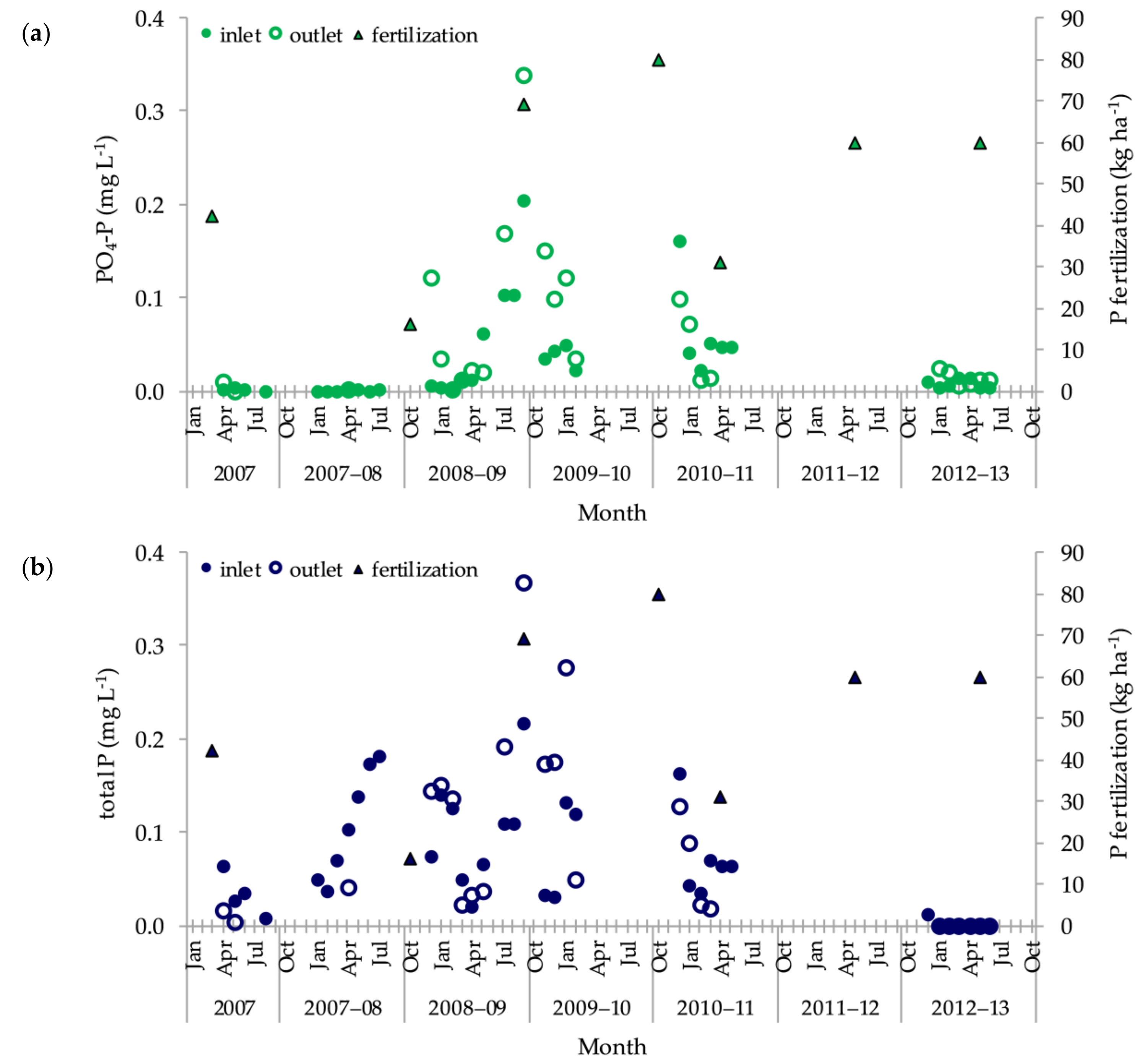
Phosphorus showed a different behavior (Figure 5) with respect to nitrogen.

An increase in total P inflow concentrations was reported during the hydrological year 2007–2008, peaking at 0.183 mg L⁻¹ in July. During that year, water was pumped into the SFCW but the floodwater never reached the riser and almost no outflows were produced. In 2008–2009, the SFCW finally received enough water to generate outlet discharge, and both PO₄–P and total P outflow concentrations increased, peaking at 0.339 mg L⁻¹ and 0.368 mg L⁻¹, respectively in September. Two phenomena could be held responsible for this: (i) water removal proceeding at a faster pace than P removal (with an increase in P concentrations in the lower water volumes that reach the outlet); (ii) mobilization of P accumulated in the basin the previous year. Indeed, as reported by Reddy et al. [34], after a long period with no outflows, all the P released by the decomposing litter and accumulated with the inflow could easily be transported to the outflow by the floodwater.

3.4. N and P Annual Concentrations

Significant differences were found between inflow and outflow NO₃–N concentrations in 2007, 2008–2009, 2009–2010, and 2010–2011 hydrological years (

Table 2. Annual inlet and outlet N and P concentrations (median and interquartile range). Data is organized into hydrological years (October–September). p-values of the Mann–Whitney nonparametric test are reported (significant differences in bold).

Year		NO3–N mg L−1	Total N mg L−1	PO4–P mg L−1	Total P mg L−1
	In	4.38 (3.51–5.89)	5.36 (4.70–7.78)	0.000 (0.000–0.001)	0.002 (0.001–0.014)
2007 a	Out	2.51 (1.63–3.13)	4.34 (3.83–6.38)	0.002 (0.000–0.007)	0.009 (0.004–0.017)
	p-value	0.000	0.078	0.086	0.160
	In	2.73 (1.08–4.94)	6.35 (4.76–8.40)	0.000 (0.000–0.000)	0.053 (0.039–0.148)
2007–08	Out	4.25 (2.57–5.98)	7.37 (5.44–8.63)	0.001 (0.000–0.043)	0.043 (0.040–0.070)
	p-value	0.331	0.803	0.462	0.543
	In	2.62 (2.09–3.90)	5.44 (4.85–7.64)	0.005 (0.003–0.012)	0.099 (0.037–0.171)
2008–09	Out	1.59 (0.59–2.93)	4.10 (2.77–7.92)	0.005 (0.004–0.011)	0.035 (0.018–0.151)
	p-value	0.008	0.102	0.479	0.426
	In	4.17 (0.95–6.76)	6.80 (3.28–9.22)	0.033 (0.015–0.065)	0.028 (0.003–0.161)
2009–10	Out	4.33 (1.27–6.84)	3.57 (0.71–9.49)	0.064 (0.017–0.102)	0.066 (0.012–0.198)
	p-value	0.928	0.552	0.304	0.321
	In	5.87 (5.33–6.28)	5.02 (4.48–5.73)	0.039 (0.015–0.095)	0.092 (0.024–0.161)
2010–11	Out	2.27 (1.43–4.03)	4.55 (3.36–5.50)	0.060 (0.015–0.110)	0.054 (0.027–0.114)
	p-value	0.002	0.481	0.743	1.000
	In	no flow	no flow	no flow	no flow
2011–12	Out	no flow	no flow	no flow	no flow
	p-value	-	-	-	-
	In	8.89 (6.82–11.10)	9.59 (7.69–11.97)	0.006 (0.001–0.013)	-
2012–13	Out	7.90 (6.71–11.15)	8.91 (7.10–11.51)	0.010 (0.000–0.015)	-
	p-value	0.522	0.459	0.409	-

^a Starting from March.

).

In 2007, vegetation started growing again after rehabilitation, and N uptake could have played a substantial role in reducing outlet concentrations of both NO₃–N (p-value < 0.05) and total N (p-value = 0.08), in accordance with what Borin and Tocchetto [16] reported for the previous period. During 2008–2009, NO₃–N concentrations were the lowest of the entire period, with a significant difference between inflow and outflow values. Indeed, rainfall in 2008–2009 was plentiful (1077 mm), and the drainage water discharge from the surrounding fields was homogeneously distributed during the year. This created the conditions for an extended residence time in the SFCW basin. Lavrnić et al. [35] reported a similar situation in a study conducted on an SFCW in a nearby Italian region with similar climatic conditions: the authors found significant differences between inflow and outflow N concentrations when the residence time was longer, due to higher infiltration and nutrient losses, and increased pollutant removal. In 2009–2010, NO₃–N inflow concentrations started to increase. In that year, N fertilization in the surrounding fields had been applied as both mineral and organic cattle slurry, at rates of up to 300 kg N ha⁻¹ year⁻¹, thus increasing the overall concentrations in drainage waters. In 2010–2011, a significant difference between inlet and outlet concentrations was reported due to effective N removal. Similar results were observed for total N, despite significant differences never being found between inflow and outflow. In fact, only slight reductions were observed in 2007, and between 2008 and 2011. In the last years, there was also a noticeable increase in the proportion of NO₃–N with respect to total N in the inflow. This is not surprising, as nitrate leaching presents a major issue in fields where maize is cultivated continuously, and cattle slurry is applied (especially in autumn) [36].

As in the case of total N concentrations, PO₄–P and total P did not show significant differences between inlet and outlet annual values. Higher P concentrations were observed in both inlet and outlet water in 2009–2010 and 2010–2011, after the switch to mixed mineral and cattle slurry fertilizations. In 2012–2013, when slurry was not applied in autumn but in late spring, P concentrations in winter water flows showed a sharp decrease, and total P values started to fall below the detection limit.

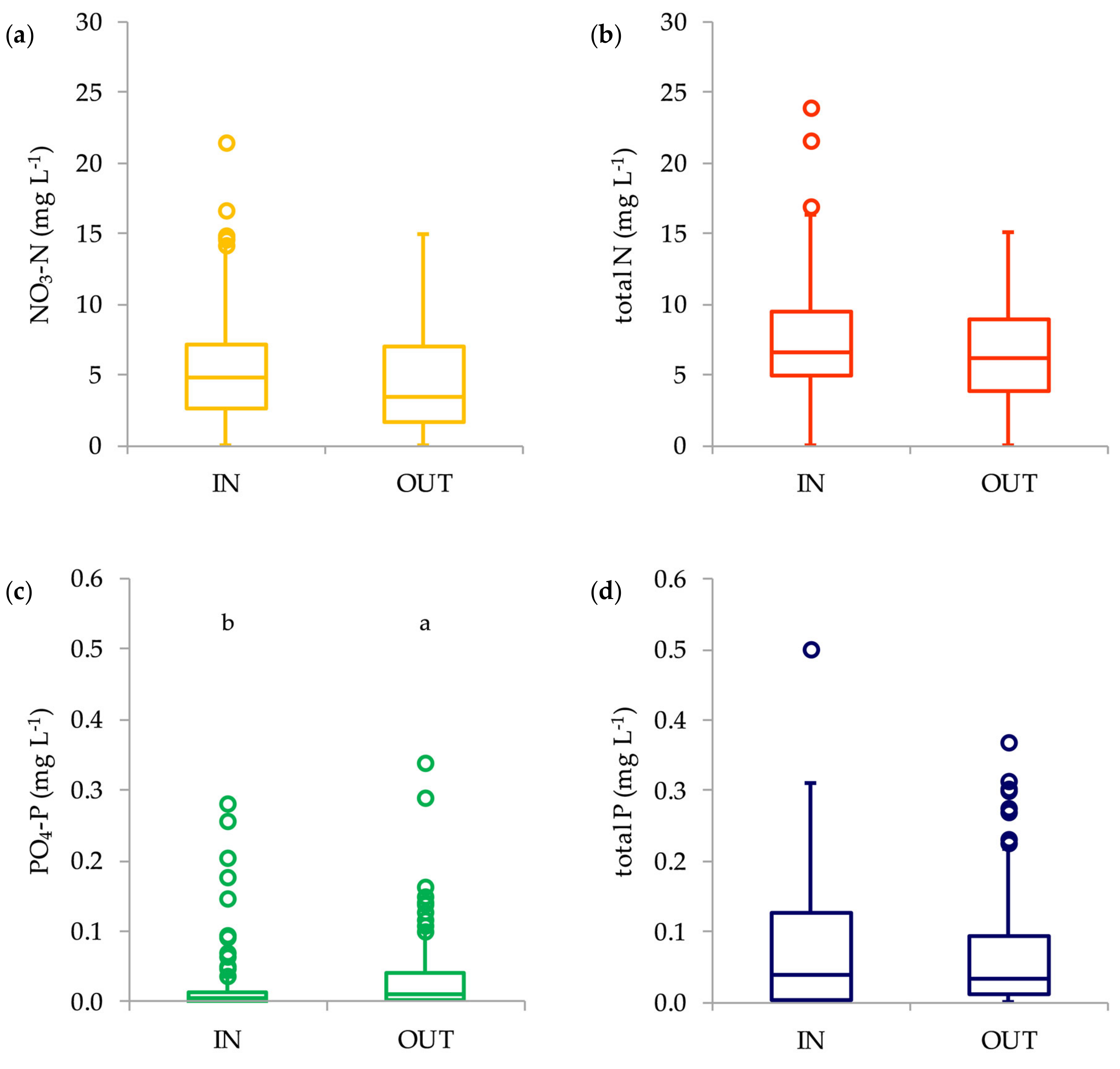
Figure 6 provides an overview of the inflow and outflow nutrient concentrations of the entire period (2007–2013). With regards to N, concentrations at the inlet were slightly higher than at the outlet, and showed more outliers, even though no significant differences were found. As for PO₄–P, concentrations were significantly greater at the outlet. Total P inflow concentrations were slightly, but not significantly, higher than outflow concentrations.

3.5. Total Nutrient Loads and Comparison with Previous Period

Nitrogen and phosphorus loads of the entire period are shown in

Table 3. SFWC nitrogen balance (NO₃–N and total N). Inlet and outlet loads, estimated lateral losses, removal ratio (R_R), and removal efficiency (R_E) are reported.

	NO3–N (kg ha−1)					Total N (kg ha−1)
Year (Oct–Sep)	Inlet Loads	Outlet Loads	Lateral Losses	RR %	RE %	Inlet Loads	Outlet Loads	Lateral Losses	RR %	RE %
2007a	93	8	3	91	88	136	16	5	88	85
2007–08	61	3	1	95	93	159	5	5	97	94
2008–09	289	29	15	90	85	639	99	58	84	75
2009–10	409	86	36	79	70	575	115	102	80	62
2010–11	569	78	11	86	84	689	111	32	84	79
2011–12	0	0	0	-	-	0	0	0	-	-
2012–13	961	170	58	82	76	1023	180	65	82	76
total	2381	374	124	84	83	3221	525	267	84	79

^a starting from March.

and

Table 4. SFCW phosphorus balance (PO₄–P and total P). Inlet and outlet loads, estimated lateral losses, removal ratio (R_R), and removal efficiency (R_E) are reported.

	PO4–P (kg ha−1)					Total P (kg ha−1)
Year (Oct–Sep)	Inlet Loads	Outlet Loads	Lateral Losses	RR %	RE %	Inlet Loads	Outlet Loads	Lateral Losses	RR %	RE %
2007 a	0.07	0.01	0.00	78	76	0.75	0.04	0.02	95	93
2007–08	0.02	0.00	0.00	97	93	2.16	0.03	0.10	99	94
2008–09	3.03	0.96	1.81	68	9	9.56	1.98	2.44	79	54
2009–10	3.24	1.80	1.34	44	3	6.59	3.18	1.79	52	25
2010–11	11.01	1.72	1.41	84	72	11.65	1.97	1.51	83	70
2011–12	0.00	0.00	0.00	-	-	0.00	0.00	0.00	-	-
2012–13	1.16	0.29	0.46	75	36	n.s.	n.s.	n.s.	-	-
total	18.53	4.79	5.01	74	48	30.71	7.19	5.87	77	67

^a starting from March.

, respectively.

During the previous study (1998–2002 period), annual total N inlet loads were on average 320 kg ha⁻¹, ranging from 43 kg ha⁻¹ to 834 kg ha⁻¹ [16]. In this study (2007–2013 period), annual total N inlet loads were generally higher, with an average of 460 kg ha⁻¹, ranging from 0 kg ha⁻¹ to 1023 kg ha⁻¹. Annual NO₃–N inlet loads were on average 340 kg ha⁻¹, ranging from 0 kg ha⁻¹ to 961 kg ha⁻¹. Nitrogen removal efficiency was 83% for NO₃–N and 79% for total N. Nitrogen removal was lower in years with higher inlet loads. Land et al. [12], in their review considering multiple studies mainly across Europe and the US, calculated a median removal efficiency of 37%. Our SFCW, though, had a fluctuating hydroperiod that produced discontinuous and reduced outflows, creating the conditions for a high N removal. As reported by Mitsch et al. [37], nutrient removal in surface flow wetlands can be sustainable for decades if loading rates are not excessive. With respect to the previous results conducted on the newly-established SFCW [16], N removal slightly decreased here. Mitsch et al. [17] reported that N retention in SFCW generally decreases with time, but they stressed that a major role is played by the hydrological pulsing. It is therefore unsafe to assume that the N retention reduction observed here was only due to the evolution of the wetland ecosystem over time, as the annual hydraulic loading in 2007–2013 was greater than in 1998–2002. Nevertheless, some positive effects on N removal related to the structural modifications made in 2007 may not be completely excluded, especially due to the creation of additional banks that likely increased the SFCW hydraulic efficiency [38].

Annual PO₄–P inlet loads were on average 2.90 kg ha⁻¹, ranging from 0 to 11.01 kg ha⁻¹. Annual total P inlet loads were on average 5.12 kg ha⁻¹, ranging from 0 to 11.65 kg ha⁻¹. Phosphorus removal efficiency was 48% for PO₄–P and 67% for total P. Values varied considerably among the years. Removal efficiencies were the lowest in 2008–2009 (9%) and 2009–2010 (3%). Fisher and Acreman [14], reviewing the performances of several wetlands around the world, reported a high range of P removal efficiency, from less than 30% to almost 100%. Of the studies that recorded the greatest reduction in P loading, however, none was conducted for more than two years. In general, long-term P retention is reported to decrease due to saturation of storage in soil, detritus, and plant biomass, but short-term fluctuations should be expected [17].

3.6. Factors Affecting Outlet Concentrations and Nutrient Removal

Starting from the full model that included monthly water inflow, monthly flow-weighted inlet concentrations, and monthly average air temperature, the stepwise procedure yielded the model with the highest likelihood for each nutrient form. Relevant parameters of the selected models are reported in

Table 5. Parameters of the selected models per each nutrient form. Whole model parameters (p-value and R squared) and predictors parameters (p-values and regression coefficients) are reported. p-values < 0.05 are in bold. Expressions in parentheses refer to Equation (4). Concentrations (monthly flow-weighted) are in mg L⁻¹; air temperature (monthly average) in °C, inflow (monthly volumes) in 10³ mm.

		Outlet Concentration (CO)
		NO3–N	Total N	PO4–P	Total P
Whole model	p-value	<0.01	<0.01	<0.01	0.07
	R2	0.63	0.60	0.33	0.19
Intercept	p-value	0.40	0.08	0.06	0.34
	coeff. (β0)	−0.64	2.25	0.02	0.04
Inflow	p-value	-	-	-	-
(WI)	coeff. (β1)
Inlet concentration	p-value	<0.01	<0.01	<0.01	0.0.7
(CI)	coeff. (β2)	0.90	0.67	0.80	0.77
Air temperature (T)	p-value	-	0.02	-	-
	coeff. (β3)		−0.11

and

Table 6. Parameters of the selected models per each nutrient form. Whole model parameters (p-value and R squared) and predictors parameters (p-values and regression coefficients) are reported. p-values < 0.05 are in bold. Expressions in parentheses refer to Equation (4). Removal ratio (monthly values) is in %; inflow (monthly volumes) in 10³ mm, inlet concentration (monthly flow-weighted) in 10³ mm, air temperature (monthly average) in °C.

		Removal Ratio (RR)
		NO3–N	Total N	PO4–P	Total P
Whole model	p-value	<0.01	<0.01	-	0.04
	R2	0.46	0.47		0.22
Intercept	p-value	<0.01	<0.01	<0.01	<0.01
	coeff. (β0)	99.93	98.31	54.83	108.20
Inflow(WI)	p-value	<0.01	<0.01	-	0.04
	coeff. (β1)	−7.80	−8.22		−24.71
Inlet concentration (CI)	p-value	-	-	-	-
	coeff. (β2)
Air temperature (T)	p-value	-	-	-	-
	coeff. (β3)

, considering monthly flow-weighted outlet concentrations and monthly removal ratios, respectively, as the output variable.

Outlet concentrations were significantly related to inlet concentrations (Table 5), with regard to NO₃–N (r² = 0.63, p-value < 0.01) and PO₄–P (r ² = 0.33, p-value < 0.01): the relationship was weaker for soluble P. Outlet NO₃–N and PO₄–P concentrations were 90% and 80% of the inlet values, respectively, highlighting an effective reduction provided by the SFCW. As for the total N model (r² = 0.60, p-value < 0.01), outlet concentrations were 67% of the inlet values, and a relationship with air temperature was also found: per each additional degree Celsius, outlet concentrations showed an overall decrease of 0.11 mg L⁻¹, probably because periods with higher temperatures are related to increased plant growth and microbial activity [6,39]. No significant relationship was found between total P outlet concentrations and the selected predictors. Inlet water loads was not a significant predictor in any case.

Removal ratios were significantly and negatively related to inlet water loads (Table 6) with regard to NO₃–N (r² = 0.46, p-value < 0.01) and total N (r ² = 0.47, p-value < 0.01). This confirmed the findings on N loads for this period (2007–2013) and the previous one (1998–2002) [16], linking quantitatively the N removal performances to the hydraulic loading. The relationship was weaker for total P (r² = 0.22, p-value 0.04), as could be expected due to the different nutrient dynamics with respect to N. Inlet flow-weighted concentrations and temperature were not selected as significant predictors affecting SFCW treatment performance. As indicated by the β₁ coefficients in Table 6, the removal ratio was linearly reduced by 7.80% (for NO₃–N), 8.22% (for total N), and 24.71% (for total P) per each 10³ mm increase in the inlet water loads; that is to say, the SFCW showed worse performances with greater hydraulic loadings. Similarly, results reviewed by Land et al. [12] showed a significant negative correlation between N removal and hydraulic loading, although the authors found wetland performances being also significantly affected by air temperature. It is worth noting, though, that Land et al. [12] included various wetlands from different climatic regions in their study, collecting a larger number of data than in our case, with greater variability in the temperature range. As for PO₄–P, no relationship was found between removal ratio and any of the investigated variables.

4. Conclusions

After 17 years of operation, the SFCW was still effective in reducing NO₃–N, total N, PO₄–P, and total P loads coming from agricultural drainage waters. PO₄–P concentrations increased at the outlet but the SFCW lowered the overall PO₄–P mass loads. With respect to the first years of operation, N removal performances were only slightly reduced despite greater water loadings. NO₃–N removal ratio and total N removal ratios were negatively related to water inflow, with a decrease of 7.80% and of 8.22% per each increase of 10³ mm of water inlet load and r² of 0.46 and 0.47, respectively. Peak in inlet N flow-weighted concentrations was reached in January 2013, with 12.19 mg L⁻¹ of NO₃–N and 12.43 mg L⁻¹ of total N. Peak in outlet P flow-weighted concentration was reached in September 2009, with 0.339 mg L⁻¹ of PO₄–P and 0.368 mg L⁻¹ of total P.

Water removal efficiency averaged at 78% for the 2007–2013 period. N removal efficiency averaged at 83% and 79% for NO₃–N and total N, respectively. P removal efficiency averaged at 48% and 67% for PO₄–P and total P, respectively. These values were higher than in many other studies, likely due to the fluctuating hydroperiod that did not put the wetland under excessive stress.

This study revealed that in our environment: (i) nutrient removal dynamics and performances were mainly influenced by hydraulic loading; (ii) although N loads were more frequent during winter due to greater drainage and leaching from surrounding fields, they were largely removed by the SFCW; (iii) higher P loads were more frequent when the early-autumn water outflows mobilized P decomposed from the wetland litter during summer.

In conclusion, the multi-year monitoring highlighted that surface flow constructed wetlands have the potential to be effectively applied as a long-term strategy in the Venice Lagoon drainage basin, increasing water storage of agricultural areas and reducing surface water pollution. As no other long-term studies of the same type have been conducted in the same region, we believe this evidence should be considered when planning the creation of surface flow constructed wetlands in our environment.

References

- Cohen-Shacham, E.; Walters, G.; Janzen, C.; Maginnis, S. Nature-Based Solutions to Address Global Societal Challenges; IUCN: Gland, Switzerland, 2016. [Google Scholar]
- Vymazal, J. Emergent plants used in free water surface constructed wetlands: A review. Ecol. Eng. 2013, 61, 582–592. [Google Scholar] [CrossRef]
- Liquete, C.; Udias, A.; Conte, G.; Grizzetti, B.; Masi, F. Integrated valuation of a nature-based solution for water pollution control. Highlighting hidden benefits. Ecosyst. Serv. 2016, 22, 392–401. [Google Scholar] [CrossRef]
- Dal Ferro, N.; Ibrahim, H.M.S.; Borin, M. Newly-established free water-surface constructed wetland to treat agricultural waters in the low-lying Venetian plain: Performance on nitrogen and phosphorus removal. Sci. Total Environ. 2018, 639, 852–859. [Google Scholar] [CrossRef]
- Kadlec, R.H.; Wallace, S. Treatment Wetlands, 2nd ed.; CRC Press: Boca Raton, FL, USA, 2008. [Google Scholar]
- Vymazal, J. Removal of nutrients in various types of constructed wetlands. Sci. Total Environ. 2007, 380, 48–65. [Google Scholar] [CrossRef]
- Gachango, F.G.; Pedersen, S.M.; Kjærgaard, C. Cost-effectiveness analysis of surface flow constructed wetlands (SFCW) for nutrient reduction in drainage discharge from agricultural fields in Denmark. Environ. Manag. 2015, 56, 1478–1486. [Google Scholar] [CrossRef] [PubMed]
- Billy, C.; Birgand, F.; Ansart, P.; Peschard, J.; Sebilo, M.; Tournebize, J. Factors controlling nitrate concentrations in surface waters of an artificially drained agricultural watershed. Landsc. Ecol. 2013, 28, 665–684. [Google Scholar] [CrossRef]
- O’Geen, A.T.; Budd, R.; Gan, J.; Maynard, J.J.; Parikh, S.J.; Dahlgren, R.A. Mitigating nonpoint source pollution in agriculture with constructed and restored wetlands. Adv. Agron. 2010, 108, 1–76. [Google Scholar]
- Woltemade, C.J. Ability of restored wetlands to reduce nitrogen and phosphorus concentrations in agricultural drainage water. J. Soil Water Conserv. 2000, 55, 303–309. [Google Scholar]
- Dunne, E.J.; Reddy, K.R. Phosphorus biogeochemistry of wetlands in agricultural watersheds. In Nutrient Management in Agricultural Watersheds—A Wetlands Solution; Dunne, E.J., Reddy, K.R., Carton, O.T., Eds.; Wageningen Academic Publishers: Wageningen, The Netherlands, 2005; Chapter 4; pp. 105–119. [Google Scholar]
- Land, M.; Granéli, W.; Grimvall, A.; Hoffmann, C.C.; Mitsch, W.J.; Tonderski, K.S.; Verhoeven, J.T. How effective are created or restored freshwater wetlands for nitrogen and phosphorus removal? A systematic review. Environ. Evid. 2016, 5, 9. [Google Scholar] [CrossRef]
- Vymazal, J. The use of constructed wetlands for nitrogen removal from agricultural drainage: A review. Sci. Agric. Bohem. 2017, 48, 82–91. [Google Scholar] [CrossRef]
- Fisher, J.; Acreman, M.C. Wetland nutrient removal: A review of the evidence. Hydrol. Earth Syst. Sci. Discuss. 2004, 8, 673–685. [Google Scholar] [CrossRef]
- Reddy, K.R.; DeBusk, T.A. State-of-the-art utilization of aquatic plants in water pollution control. Water Sci. Technol. 1987, 19, 61–79. [Google Scholar] [CrossRef]
- Borin, M.; Tocchetto, D. Five year water and nitrogen balance for a constructed surface flow wetland treating agricultural drainage waters. Sci. Total Environ. 2007, 380, 38–47. [Google Scholar] [CrossRef] [PubMed]
- Mitsch, W.J.; Zhang, L.; Stefanik, K.C.; Nahlik, A.M.; Anderson, C.J.; Bernal, B.; Hernandez, M.; Song, K. Creating wetlands: Primary succession, water quality changes, and self-design over 15 years. Bioscience 2012, 62, 237–250. [Google Scholar] [CrossRef]
- Bendoricchio, G.; Calligaro, L.; Carrer, G.M. Consequences of diffuse pollution on the water quality of rivers in the Watershed of the Lagoon of Venice (Italy). Water Sci. Technol. 1999, 39, 113–120. [Google Scholar] [CrossRef]
- Carpani, M.; Giupponi, C.; Trevisiol, P. Evaluation of agri-environmental measures in the Venice Lagoon watershed. Nitrogen budgets and surplus indicators. Ital. J. Agron. 2008, 3, 167–182. [Google Scholar] [CrossRef]
- Dal Ferro, N.; Cocco, E.; Berti, A.; Lazzaro, B.; Morari, F. How to enhance crop production and nitrogen fluxes? A result-oriented scheme to evaluate best agri-environmental measures in Veneto Region, Italy. Arch. Agron. Soil Sci. 2018, 11, 1–16. [Google Scholar] [CrossRef]
- European Commission (EC). Council Directive Concerning the Protection of Waters against Pollution Caused by Nitrates from Agricultural Sources (1991/676/EEC); European Commission: Brussels, Belgium, 1991. [Google Scholar]
- European Commission (EC). Council Directive Establishing a Framework for Community Action in the Field of Water Policy (2000/60/EC); European Comision: Brussels, Belgium, 2000. [Google Scholar]
- Grizzetti, B.; Pistocchi, A.; Liquete, C.; Udias, A.; Bouraoui, F.; van De Bund, W. Human pressures and ecological status of European rivers. Sci. Rep. 2017, 7, 205. [Google Scholar] [CrossRef] [PubMed]
- Rubel, F.; Brugger, K.; Haslinger, K.; Auer, I. The climate of the European Alps: Shift of very high resolution Köppen-Geiger climate zones 1800–2100. Meteorol. Z. 2017, 26, 115–125. [Google Scholar] [CrossRef]
- IUSS Working Group WRB. World Reference Base for Soil Resources 2014—International Soil Classification System for Naming Soils and Creating Legends for Soil Maps; World Soil Resources Reports No. 106; FAO: Rome, Italy, 2014. [Google Scholar]
- Passoni, M.; Morari, F.; Salvato, M.; Borin, M. Medium-term evolution of soil properties in a constructed surface flow wetland with fluctuating hydroperiod in North Eastern Italy. Desalination 2009, 246, 215–225. [Google Scholar] [CrossRef]
- Berti, A.; Tardivo, G.; Chiaudani, A.; Rech, F.; Borin, M. Assessing reference evapotranspiration by the Hargreaves method in north-eastern Italy. Agric. Water Manag. 2014, 140, 20–25. [Google Scholar] [CrossRef]
- APAT-IRSA/CNR. Metodi Analitici per le Acque; Manuali e Linee Guida; APAT: Rome, Italy, 2003; Volume 29, ISBN 88-448-0083-7. [Google Scholar]
- Tolomio, M.; Borin, M. Water table management to save water and reduce nutrient losses from agricultural fields: 6 years of experience in North-Eastern Italy. Agric. Water Manag. 2018, 201, 1–10. [Google Scholar] [CrossRef]
- Borin, M.; Morari, F.; Bonaiti, G.; Paasch, M.; Skaggs, R.W. Analysis of DRAINMOD performances with different detail of soil input data in the Veneto region of Italy. Agric. Water Manag. 2000, 42, 259–272. [Google Scholar] [CrossRef]
- Barco, A.; Maucieri, C.; Borin, M. Root system characterization and water requirements of ten perennial herbaceous species for biomass production managed with high nitrogen and water inputs. Agric. Water Manag. 2018, 196, 37–47. [Google Scholar] [CrossRef]
- Shmueli, G. To explain or to predict? Stat. Sci. 2010, 25, 289–310. [Google Scholar] [CrossRef]
- R Core Team. R: A Language and Environment for Statistical Computing; R Foundation for Statistical Computing: Vienna, Austria, 2018; Available online: https://www.R-project.org/ (accessed on 17 December 2018).
- Reddy, K.R.; Kadlec, R.H.; Flaig, E.; Gale, P.M. Phosphorus retention in streams and wetlands: A review. Crit. Rev. Environ. Sci. Technol. 1999, 29, 83–146. [Google Scholar] [CrossRef]
- Lavrnić, S.; Braschi, I.; Anconelli, S.; Blasioli, S.; Solimando, D.; Mannini, P.; Toscano, A. Long-term monitoring of a surface flow constructed wetland treating agricultural drainage water in Northern Italy. Water 2018, 10, 644. [Google Scholar] [CrossRef]
- Paul, J.W.; Zebarth, B.J. Denitrification and nitrate leaching during the fall and winter following dairy cattle slurry application. Can. J. Soil Sci. 1997, 77, 231–240. [Google Scholar] [CrossRef]
- Mitsch, W.J.; Zhang, L.; Waletzko, E.; Bernal, B. Validation of the ecosystem services of created wetlands: Two decades of plant succession, nutrient retention, and carbon sequestration in experimental riverine marshes. Ecol. Eng. 2014, 72, 11–24. [Google Scholar] [CrossRef]
- Su, T.M.; Yang, S.C.; Shih, S.S.; Lee, H.Y. Optimal design for hydraulic efficiency performance of free-water-surface constructed wetlands. Ecol. Eng. 2009, 35, 1200–1207. [Google Scholar] [CrossRef]
- Mietto, A.; Politeo, M.; Breschigliaro, S.; Borin, M. Temperature influence on nitrogen removal in a hybrid constructed wetland system in Northern Italy. Ecol. Eng. 2015, 75, 291–302. [Google Scholar] [CrossRef]
Figure 1.
(a) Surface flow constructed wetlands (SFCW) scheme. The pump of the wetland is located on the south-western corner (dark blue circle). Dark blue arrows represent the inlet and the outlet. The three banks inside the basin force water to follow the path indicated by the light blue arrows. The black dot in the middle indicates the position of the phreatimeter (b) photo of the SFCW at the inlet (south-western corner) during winter.
Figure 2.
(a) Monthly rainfall and reference evapotranspiration (Hargreaves); median, 25th, and 75th percentiles are reported. (b) Annual rainfall and reference evapotranspiration; hydrological years (October–September) from 2006–2007 to 2012–2013 are considered.
Figure 3.
(a) Monthly air temperature at 2 m height (mean, minimum, and maximum temperatures are reported). (b) Annual air temperature at 2 m height (mean, minimum and maximum temperatures are reported); hydrological years (October–September) from 2006–2007 to 2012–2013 are considered.
Figure 4.
NO3–N (a) and total N (b) monthly flow-weighted inlet and outlet concentrations. N fertilizer applications are reported.
Figure 5.
PO4–P (a) and total P (b) monthly flow-weighted inlet and outlet concentrations. P fertilizer applications are reported.
Figure 6.
Nutrient inflow (IN) and outflow (OUT) concentrations of the entire period (2007–2013). (a) NO3–N; (b) total N; (c) PO4–P; (d) total P. Different letters indicate a significant difference detected by the Mann–Whitney test.