
Machine Learning Prediction of Biomarkers from SNPs and of Disease Risk from Biomarkers in the UK Biobank


1
Department of Physics and Astronomy, Michigan State University, 567 Wilson Rd, East Lansing, MI 48824, USA
2
Genomic Prediction, Inc., 675 US Highway One, North Brunswick, NJ 08902, USA
*
Authors to whom correspondence should be addressed.
Genes 2021, 12(7), 991; https://0-doi-org.brum.beds.ac.uk/10.3390/genes12070991
Submission received: 30 March 2021
/
Revised: 22 June 2021
/
Accepted: 23 June 2021
/
Published: 29 June 2021
(This article belongs to the Special Issue Application of Genomic Technology in Disease Outcome Prediction)
Abstract
:We use UK Biobank data to train predictors for 65 blood and urine markers such as HDL, LDL, lipoprotein A, glycated haemoglobin, etc. from SNP genotype. For example, our Polygenic Score (PGS) predictor correlates ∼0.76 with lipoprotein A level, which is highly heritable and an independent risk factor for heart disease. This may be the most accurate genomic prediction of a quantitative trait that has yet been produced (specifically, for European ancestry groups). We also train predictors of common disease risk using blood and urine biomarkers alone (no DNA information); we call these predictors biomarker risk scores, BMRS. Individuals who are at high risk (e.g., odds ratio of >5× population average) can be identified for conditions such as coronary artery disease (AUC∼0.75), diabetes (AUC∼0.95), hypertension, liver and kidney problems, and cancer using biomarkers alone. Our atherosclerotic cardiovascular disease (ASCVD) predictor uses ∼10 biomarkers and performs in UKB evaluation as well as or better than the American College of Cardiology ASCVD Risk Estimator, which uses quite different inputs (age, diagnostic history, BMI, smoking status, statin usage, etc.). We compare polygenic risk scores (risk conditional on genotype: PRS) for common diseases to the risk predictors which result from the concatenation of learned functions BMRS and PGS, i.e., applying the BMRS predictors to the PGS output.
1. Introduction
Modern machine learning (ML) methods have opened the door to using high dimensional inputs to predict health outcomes and risk. This paper concerns the application of sparse linear ML to genetic and health information in order to make predictions that could be useful in a clinical setting. Recent work has highlighted that ML, in particular polygenic predictors, have high potential impact in clinical settings [1,2,3,4,5,6,7,8,9,10,11,12,13,14,15,16,17,18,19,20,21], especially for coronary artery disease (CAD) [11,12,22]. Additionally, over the past quarter century it has been advocated (e.g., Joint Task Force of the European Society of Cardiology and Other Societies [23], American College of Cardiology(ACC)/American Heart Association (AHA) [24], and the Scottish Intercollegiate Guidelines Network [25]) that physicians should use risk scores based on statistical summaries of biomarkers. Examples of such scores include Framingham [26,27], SCORE [28], ASSIGN–SCORE [29], QRISK1 [30], QRISK2 [31], QRISK3 [32], PROCAM [33], Pooled Cohort Studies Equations [34,35,36], CUORE [37], Globorisk [38], Reynolds risk score [39,40], World Health Organization (WHO) risk chart [41,42], MyRisk_stroke calculator [43], NIPPON [44], and UKPDS risk engine [45,46].
In [47] it was emphasized that cardiovascular disease (CVD) risk scores have a long history. Although early attempts to identify key genetic risk markers had some missteps, Reference [47] argues that—thanks to new methods and larger datasets—genetic risk scores have developed enough to begin being employed in clinical practice (e.g., [22]). Additionally, [48] charts the rise of ML/AI in cardiology in general and predicts that it will play a major role in diagnostic and precision medicine involving cardiology.
Some examples of using ML to predict CVD risk include: In [49] biomarkers—(apo)lipoproteins and cholesterols—were used with a Cox-hazard-model to claim that Total Cholesterol and HDL are sufficient for good CVD risk assessment. Apolipoproteins, LDL, and other lipids in general offered very modest improvements in risk prediction with this model (some of this is medication, e.g., statin, dependent); in [50] a convolutional neural network and gradient boosting algorithms were used on a small subset of biomarkers, imaging results, and medical history (including ASCVD risk score) on a sample size of ∼2000 to predict myocardial infarction (heart attack) and death. Including all variables the approach reached an Area Under the Receiver operator characteristic Curve (AUC) ( CI: 77–87); in [51] a support vector machine learning algorithm was used and showed out-performance over the ACC/AHA pooled cohort studies equations. This was measured by recommending less drug therapy while missing fewer events of CVD; in [52] a support vector machine learning classifier algorithm was trained on pre-selected biomarkers, medical and family history, and imaging data. This approach was then compared to standard “statistical scores” for CVD such as Framingham [26,27], SCORE [28], QRISK3 [32], PROCAM [33], Pooled Cohort Studies Equations [34,36], CUORE [37], Globorisk [38], Reynolds risk score [39,40], World Health Organization (WHO) risk chart [41,42], MyRisk_stroke calculator [43], NIPPON [44], and UKPDS risk engine [45,46]. Additional examples of using ML primarily on single nucleotide polymorphism (SNP) data include: in [12], LDpred [53] was used to predict coronary artery disease (CAD) and found, using additional common covariates like age and sex, an AUC∼0.81 ( CI: 0.80–0.81 ); using only SNP information, in [11] a sparse ML approach was used to predict heart atrial fibrillation (AUC∼0.64), hypertension (AUC∼0.65), and heart attack (AUC∼0.59); and in [22] a meta-analysis was done to generate a hazard ratio (HR) for CAD of 1.71 ( CI: 1.68–1.73). AUC has become a standard metric for evaluating polygenic scores for disease risk. However, one of the most promising applications of these scores is their ability to identify risk outliers, as highlighted in [11,54]. Outlier identification often works well, even for predictors with only moderately strong AUCs.
This work applies ML to both SNP based prediction and biomarker based prediction. We focus on a type of sparse ML (LASSO) which does feature selection, as well as relative weighting. In other words, sparse ML selects a subset of all the possible variables and then gives them relative weights. This is in contrast to most of the statistical methods used above where the inclusion of biomarkers relied mostly on previous research on the biomarkers themselves. In addition to feature selection, this sparse approach has been chosen because of previous success with SNP based prediction [11,54,55,56,57,58,59] and because it has been shown to be among the best ML predictors for genetics and is often a good all around method [56,60].
The source of data for this work is the UK Biobank (UKB) [61], which includes SNP genotypes, medical diagnosis information, and extensive biomarker information (i.e., 65 quantitative outputs of blood and urine tests) for almost 500 k individuals. In this article, we describe sparse ML investigations of the correlation structure between these three categories of data. As described in Figure 1, we train:
- 1. PGS
- Polygenic Score (PGS) predictors of the quantitative biomarker test results from SNPs alone. These functions predict biomarker level conditional on genotype: PGS.For example, we predict measured lipoprotein A levels from SNPs, achieving a correlation of 0.76 between PGS and actual biomarker level. The goal with this training is to study how accurately biomarker levels can be predicted, to investigate the underlying genetic architecture, and to be used as input for the predictors in point 3 below.
- 2. BMRS
- Biomarker Risk Scores (BMRS) which predict risk of a specific disease condition using only measured biomarkers as input: BMRS.For example, our atherosclerotic cardiovascular disease (ASCVD) predictor uses ∼10 blood biomarkers to predict disease risk. We show that in UKB validation it predicts disease risk as well as, or better than, the American College of Cardiology ASCVD Risk Estimator [62,63], which uses quite different inputs, such as age, diagnostic history, body mass index (BMI), smoking status, statin usage, etc. Liver and kidney problem risk prediction from biomarkers seems quite promising, based on our results. In total, we investigate predictions for ASCVD, CAD, diabetes type I and II, hypertension, very inclusive definitions of kidney and liver problems, and obesity.
- 3. gBMRS and PRS
- Finally, by concatenating the predictors in 1 and 2 above, we build functions which map genotype (SNPs) to disease risk, with biomarkers as an intermediate step. We denote these concatenated predictors as: Genetic Biomarker Risk Scores (gBMRS). We emphasize that concatenation (i.e., ) is not the same as training with both biomarkers and SNPs simultaneously used as features. The concatenated predictors only require SNPs as input, but use SNP predicted biomarker values as an intermediate step in calculation of the predicted disease risk. These functions can be compared to standard Polygenic Risk Scores (PRS) computed directly from SNPs, using disease case status as the training phenotype: PRS.For example, the concatenated function which maps SNPs → biomarkers → type 2 diabetes risk performs roughly, as well as the PRS for type 2 diabetes ( AUC ∼ 0.64).We study this concatenation to see whether this alternative path to disease prediction can provide additional gains relative to the more straight-forward standard PRS.
To conform to the standard journal section structure, these three related but separate predictor types are discussed in a staggered disposition throughout the Materials and Methods and Results sections.
From our investigations, we conclude that many biomarker levels are not just substantially heritable, but can be predicted with some accuracy from SNPs. This is true despite the fact that levels fluctuate from day to day for a specific individual. We also conclude that disease risk prediction from biomarkers alone, via BMRS, is potentially very powerful, and indeed complementary to existing methods for risk estimation. For example, we show below that the ASCVD Risk Estimator uses different and complementary information to the biomarkers used in our ASCVD BMRS. Our results suggest that combining this complementary information can lead to stronger prediction and perhaps new insights into heart disease. Significant analyses of the costs and benefits of additional inputs have been performed for the existing ASCVD predictor, which is in clinical use (e.g., [62,63]), including some of the features in our predictor. Our comparison is limited to risk predictor performance and in the UKB cohort only.
We validate all predictors using sibling data: most of the power to differentiate between siblings (either in quantitative trait values or disease risk) persists despite similarity in childhood environments. We also test the fall off in power in distant ancestries (relative to the European training population). The decline for SNP based predictors varies as expected with genetic distance, whereas biomarker prediction does not display this pattern.
Throughout this paper, we refer to the different biomarkers according to the abbreviations listed in Table 1.
2. Materials and Methods
We outline here common features and methods that are used throughout this project. Later, in subsections below, we will detail the specifics that are unique to each sub-analysis.
- Subject data
All research in this paper uses data exclusively from the 2018 UKB release [61,64] and updates (see Supplementary Information for more details). All statements about sex or ancestry refer to the self-reported data within this dataset [65]. There is of course a complicated genetic substructure within each one of these subgroups [66,67,68,69,70,71,72,73,74,75,76,77,78,79]. However, previous research has demonstrated that—when looking at the UK Biobank, using sparse methods and looking at heart and blood related phenotypes—self-report can provide sufficiently good data for training purposes [54,55,56,57,58]. Genetic prediction in general depends on non-trivial factors including population substructure, size of training sets, algorithms (e.g., sparse vs non-sparse methods), heritability, environmental factors, and etc. Nonetheless, in some instances self-reported identity is sufficient for training. Sparse, self-reported training in the UKB has been compared to analyses regressing on principal components (PC) [55], compared to training and testing across adjacent ancestry groups as defined by PCs [11,80], and detailed sibling tests [58]. For the purposes of this paper, we compared predictors trained on self-reported ancestry vs regressing on residuals from a principal component analysis (PCA) where we find the results differ by ∼1% (additional details in the results section). Additionally, using a principal component analysis to account for population substructure can be problematic on small sample sizes (e.g., [81]). In order to further demonstrate that population substructure has negligible effect on the presented prediction power, we also use a sibling validation method [58]: All sets of siblings are withheld from training and used for final testing. Environmental background, such as life style and diet, and indirect genetic effects have impacts on most of the biomarkers and siblings generally have more similar backgrounds than randomly chosen pairs, and are also more genetically similar than unrelated individuals. Retained predictive power among siblings is, hence, a strong indication of direct genetic effects. Moreover, the amount of lost power as compared to the general population can give some idea of the magnitude of environmental effects, e.g., from childhood environment. (There can also be genetic nurture [82,83,84,85,86] effects that are not analyzed here).
We refer to the self-reported ancestries labeled white, Asian, Chinese, and black in UKB as European, South-Asian, East-Asian, and African, in accordance with the guidelines in [87]. It has been repeatedly confirmed that the power of polygenic predictors is dependent on both the training and testing ancestries, and that generally the power of the prediction falls off as a function of genetic distance [88,89,90,91]. All individuals with self-reported admixture were excluded from this study.
- Phenotype data
The phenotypes included in the paper include self-reported UKB statuses, biomarker measurements (sometimes repeated), standard (ICD9, ICD10, OPCS3, OPCS4) codes, diagnosed conditions, thresholds, and combinations of all the previous items. Full details of how each phenotype is defined is given in the Supplementary Information.
- Genotype data
The UKB genotype data were quality controlled by excluding all SNPs with less than 3% call success rate and also those with a minor allele frequency (MAF) <0.001. All individuals with less than 3% successfully called SNPs were also excluded and, again, any individual with self-reported mixed ancestry was excluded from this study entirely. Furthermore, only autosomal genetic information was used, including SNPs located on chromosomes 1–22 only.
- Algorithms/Machine Learning
This work primarily focuses on LASSO [92], or compressed sensing [93,94,95,96]. LASSO was chosen because it has been repeatedly shown that sparse, linear methods are among the most successful in genetic prediction over a wide variety of traits [11,55,58]. Additionally, sparsity makes application and analysis of the predictors much more computationally efficient. As genetic predictors move into clinical settings, it will undoubtedly be the case that optimal prediction algorithms will vary depending on phenotype and training data, but LASSO currently serves as an excellent jack-of-all-trades.
- Statistical evaluation
The LASSO predictors were evaluated with cross-validation. The validation set for each fold was used to choose optimal values of the regularization parameter (see Supplementary Information). The UKB subjects were divided according to self-reported ancestry and the European subset was then split into siblings as evaluation set and non-siblings as training set. The resulting training set was then split into five cross-validation folds, as shown in Figure 2. The top performing predictor—as measured by performance in the European corresponding validation set—from each fold was retained providing some statistics for the uncertainty estimates in the results. More details can be found in the Supplementary Information.
We now present in separate subsections the detailed methods used for PGS, BMRS and gBMRS, respectively, and we end with the methods for comparing our ASCVD predictor with the clinically employed ASCVD Risk Estimator.
2.1. PGS: Predicting Biomarkers from SNPs
We used LASSO to predict the 65 types of biomarkers listed in Table 1 from SNP data, and refer to these type of predictors as PGS.
Data and pre-processing: UKB contains data from repeated visits and for samples with more than one measurement of a certain biomarker the average value was taken in order to measure the heritable levels rather than fluctuations. These raw measurements were z-scored for men and women separately and consecutively age corrected by subtracting a linear regression on age-biomarker data obtained from averaging the biomarker value for all samples born the same year (biomarker-age plots are contained in Supplementary Information). The parameters for the pre-processing were determined from training sets with about 340 k samples of European ancestry. Evaluation sets of about 20–40 k European siblings and all non-European individuals were withheld entirely from training but pre-processed with the same parameters.
Predictor training: Five LASSO predictors were trained on each biomarker. Validation sets were made from randomly drawing 1000 samples and excluding these from the training set.
As a separate check for population structure, we adjusted phenotypes based on a linear regression on the 20 first principal components (as provided by UKB) of the genotypes. This was done for five of the biomarker predictors which correlated highly with the original phenotypes. We then trained LASSO predictors on the residuals. This had negligible effect (∼1%) as shown below in the result section.
Evaluation: Predictors were judged based on the correlation between predicted and measured biomarkers. Each predictor, for each biomarker and cross-validation fold, was evaluated on its corresponding evaluation set consisting of ∼20–40 k samples of European siblings. To test the performance dependence on ancestry we also applied the predictors to the 9 k of South-Asian, 1500 of East-Asian, and 7 k of African ancestry. In Section 3.2.2, we report the correlation between the PGS and the phenotypes as the performance metric for these continuous traits. The sibling evaluation consisted of calculating, for pair of samples, the difference in phenotype and the difference in PGS and comparing the correlations between these quantities within random and sibling pairs, respectively.
Genetic architecture: One can define the variance accounted for by each SNP i in a predictor according to
where is the MAF of SNP i and is the corresponding coefficient size. This is described in greater detail in the Supplementary Information and in [57]. We use this alongside Manhattan-plots of the effect sizes in the results (Section 3.1.1) to display the genetic architectures of the top 3 performing PGS predictors. Analogous plots for the rest of the PGS predictors are contained in the Supplementary Information.
2.2. Methods for Disease Prediction: BMRS and gBMRS
We used two approaches to investigate whether biomarkers can be used to predict disease risk, analogous to how blood tests are used clinically.
- 1. BMRS
- We trained predictors with LASSO to predict case/control status directly from phenotypes, i.e., using the direct biomarker measurements as features. We denote this type of predictor as biomarker risk score (BMRS).
- 2. gBMRS
- Second, we applied the already trained BMRS predictors to the predicted phenotypes, i.e., using the biomarker PGS output from the SNP-based predictors in Section 2.1 as input. As such, we obtain disease risk scores using only SNP data as input. We denote these concatenated predictors as genetic biomarker risk scores (gBMRS).
We evaluated this strategy on eight different condition definitions and we present the details for the two approaches separately. This is done both to display the performance dependence on the two approaches and since the predictions from biomarkers are very interesting in their own right.
2.2.1. BMRS: Predicting Case Status from Biomarkers
Condition definitions: Based on the available UKB data, we defined conditions for CAD, cancer, diabetes type 1, diabetes type 2, hypertension, kidney problem, liver problem, and obesity. The detailed definitions for each one of these are to be found in the Supplementary Information. In general, we chose the definitions to be inclusive; kidney (liver) problem for example contains almost all kidney (liver) related problems that are reported in UKB, whereas cancer refers to any type of cancer. Obesity was defined as a BMI over 30. The effects of changing definitions are further discussed in Section 4.
Predictor training: We used 62 out of the 65 biomarkers as input features, dropping E2, MA, and RF due to few available measurements, and taking the first available measurement for each sample (we did not use averages for the BMRS to closer resemble a clinical setting). The raw data were pre-processed by sex specific z-scoring and then age correcting by subtracting a linear regression. Using LASSO, we then trained 5 predictors on the case/control status, choosing optimal by five-fold cross-validation. The training was done separately for men (N = 106,656) and women (N = 86,193) and on European ancestry only.
We again conducted a separate check for population structure, by training on the residuals after subtracting a linear regression on the 20 first principal genotype components from the phenotypes. As for the PGS, this had no significant effect (∼1%).
Evaluation: As was done for the PGS in Section 2.1, about 40 k siblings of European ancestry and all non-European individuals were kept separate from all training and were used as evaluation sets. We measured the predictor performance by AUC and by odds ratio plots. We conducted additional sibling tests for the BMRS predictors to test for environmental effects: we applied the predictors to pairs of siblings with precisely one case and one control and report the fraction of correctly called affected sibling, juxtaposed with the same results for random pairs of one case and one control.
It should be emphasized here that we did not take the date of onset into account in this study: disease status was considered on a “life span” (as far as UKB covers) basis such that cases could have onsets both prior to and after the time of the biomarker measurement. Prediction in this sense means what can we predict about current or future case status only knowing a set of momentary biomarker values. Temporal prediction tests (i.e., prospective prediction) are deferred to later work. The distributions of time differences between condition onsets and the first biomarker measurement can be found in the Supplementary Information.
2.2.2. gBMRS: Predicting Case Status from PGS of Biomarkers
To form predictors taking SNP data as input, we concatenated the PGS predictors from Section 2.1 with the biomarker predictors BMRS to form what we call gBMRS. The BMRS disease predictors were taken as is and applied to the z-scored PGS output of the predictors in Section 2.1. No further training was done and the performance was evaluated as for and compared with the BMRS predictors.
2.3. Comparison with ASCVD Risk Estimator
Finally, for the Materials and Methods section, we describe the method of comparison between our ASCVD BMRS predictor and the ASCVD Risk Estimator [63]. The latter is a widely used tool to aid clinicians in risk estimations of and preventative care against atherosclerotic cardiovascular disease. We used this well-established resource for an exemplifying benchmark of BMRS predictors by training a predictor on this condition specifically. ASCVD aggregates several sub-diagnoses and exists in different versions. Hard ASCVD includes acute coronary syndromes, death by coronary heart disease, a history of myocardial infarction, and fatal and non-fatal stroke. A more general (extended) ASCVD definition additionally includes stable or unstable angina, coronary or other arterial revascularization, transient ischemic attack, and peripheral arterial disease presumed to be of atherosclerotic origin. We used a UKB specific extended definition, detailed in the Supplementary Information. The ASCVD Risk Estimator requires the input: age, sex, race, systolic and diastolic blood pressure, total cholesterol, HDL, LDL, history of diabetes, smoking status, time since quit smoking (if applicable), whether on hypertension treatment, whether on a statin, and whether on aspirin. It can also use previous data for follow-ups but we restricted our analysis to “first visit patients” only. All of these data fields can be found in some form in the UKB (the exact field choices are listed in the Supplementary Information).
The outputs of the ASCVD Risk Estimator are (up to) three risk estimates: 10 year risk, lifetime risk, and optimal risk, all given as a percentage. Since our UKB data only cover approximately 10 years from the first biomarker measurement, we exclusively used the 10 year risk output. We applied the underlying function of the ASCVD Risk Estimator to the corresponding data in UKB and obtained a 10 year risk estimate for 358,650 individuals for whom we also had an ASCVD case/control status. Strictly speaking, the ASCVD Risk Estimator was developed for North American cohorts and based on hard ASCVD but, as seen in Section 3.3, performed very well also in the cohorts of the UKB using the extended definition. Note, however, the current comparison is intended as an illustration of the power of BMRS and not as a rigorous test for deployment (see the Discussion below).
We then trained a BMRS predictor on case/control status, analogously to Section 2.2, but using ordinary linear regression on the z-scored biomarker measurements. This outputs a risk score which we mapped to absolute risk estimates in percentages as follows. The risk scores obtained from applying the predictor on the training data were binned and, within each bin, the disease prevalence was calculated from the case/control statuses as an estimated risk for samples with the corresponding risk scores. This discrete mapping was then made continuous using rolling averages and linear interpolation. For details see Supplementary Information.
Combination of Predictor from Biomarkers and the ASCVD Risk Estimator
In the results Section 3.3, we show that the ASCVD BMRS predictor and the ASCVD Risk Estimator are making complementary predictions. We, therefore, also tested a combination of them. We made a linear regression on all the input features from the two predictors combined (65 continuous and 8 discrete variables), z-scoring the discrete variables from the ASCVD Risk Estimator input such that everything was on the same scale. In addition, we made a second regression also including the output of the ASCVD Risk Estimator to capture the non-linearities within that function. These regressions were made and evaluated on the same training and evaluation sets as for the BMRS predictors.
3. Results
As with the section of Materials and Methods, we present the results for PGS, BMRS, gBMRS, and the ASCVD comparison in separate subsections.
3.1. Predicting Biomarkers from SNPs
The performance of the PGS predictors ranges from the highest phenotype-PGS correlation for a polygenic predictor we are aware of to no predictive power whatsoever. We present the results in order of correlation within European ancestry in Figure 3. The best performing predictor is for lipoprotein A at a correlation of ∼0.76. This is not too surprising as lipoprotein A levels are well-known to be highly heritable [97,98,99,100], related to the LPA gene and other loci [101,102,103,104,105,106,107,108,109,110], and, thus, do not greatly vary by life style or environment. Lipoprotein A has long been studied because of its association with CAD, atherosclerotic risk, liver problems, metabolism, and even cancer. Further discussion can be found in the review [111]. Yet, it is a striking example of predictive power: previous PGS have found much lower correlations for other traits. For example, height (∼0.62 [55,112]), BMI (∼0.35 [54,112], ∼0.30 [15]), educational attainment (∼0.27 [55], ∼0.35 [113]), and heel bone density (∼0.45 [55], ∼0.42 [114]). After lipoprotein A, we find correlations almost evenly distributed within the correlation range 0.1 to 0.59 and a group of 7 almost uncorrelated biomarkers at the bottom. In the same Figure 3, we have included the performance within the non-European ancestries. Being trained on European ancestry only, the predictors suffer the now familiar [90,91] fall-off pattern according to genetic distance, with performance generally being successively worse for South-Asian, East-Asian, and African ancestries.
To account for population stratification we took a two-fold approach: comparing prediction with and without adjusting for a principal component analysis, and performing sibling analyses. We used the UKB provided principal components for each individual for this analysis. We performed a linear regression on phenotype using the top 20 principal components while excluding the testing set (siblings). To assess the impact of principal components on the PGS, we compared the correlation between (1) phenotype (y) and predicted phenotype () from PCA (corr) (2) phenotype and PGS generated from training on the raw phenotype (corr) (3) the correlation between phenotype and PGS generated from training on the residual phenotype (corr). This was done for 5 out of the strongest performing predictors. The results are shown in Table 2 for the evaluation set of self-reported European individuals within sibling pairs.
From the results in Table 2 we can characterize the difference between training with and without PCA as the square root of the average difference squared
or as an average percent difference
The results from the sibling comparison can be seen in Figure 4. On average, there is a ∼26% drop in correlation when comparing differences within random pairs and differences within sibling pairs. The figure also shows that siblings that are separated by more than 0.5, 1.0, and 1.5 times the standard deviation in phenotype are predicted with increased correlation. The sibling comparisons for the other biomarkers can be found in the Supplementary Information.
3.1.1. Genetic Architecture
Polygenic predictors have shown to usually use information spread over the entire genome, even when enforcing sparsity [11,55,56,57]. In Figure 5, we illustrate the genetic architectures behind three of the top performing PGS predictors with Manhattan plots of the effect sizes and the variance accounted for in Equation (1), accumulated across chromosomes 1–22 (the Supplementary Information contains figures for all biomarkers). It shows that both biomarkers with a few very strong loci and biomarkers with an evenly distributed dependence can be predicted well. Let us make a few remarks on the top 5 performing predictors (see Supplementary Information for the direct bilirubin and platelet count plots):
- The lipoprotein A predictor is as expected heavily dominated by the single locus on chromosome 6, the gene carrying its name LPA;
- The total bilirubin predictor is very similar to the one for direct bilirubin. GWASes have implicated many variants on all but chromosome 15 (according to a GWAS Catalog [115] trait search) but most have a very minor impact on our predictor. For example, Reference [116] reported a locus on chromosome 19 but although there are groups of moderately large in this region, the entire chromosome 19 does not account for more than ∼1% of total variance in our predictors;
- GWASes for direct bilirubin in the literature [116,117] are generally dominated by variants in gene UGT1A on chromosome 2. The LASSO predictors pick these up too. In addition, there is another ∼17% variance accounted for by the locus at chromosome 12, also known [117]. Chromosomes 6 and 19 account for ∼1% variance each and have no generally listed loci. The with the largest magnitude corresponds to SNP rs908327 on chromosome 1. It has SNPs in linkage disequilibrium (LD) that have been linked to triglycerides [118] but not directly to bilirubin, to our knowledge. It has a very small MAF, however, and does not account for much variance;
- The predictor for platelet count is very polygenic with the variance accounted for almost evenly distributed across all 22 chromosomes. Chromosome 12 provides a small deviation from this pattern, accounting for ∼ of the variance, partly due to a locus near one end;
- The predictor for HDL is also highly polygenic. Previous GWASes have recorded loci at all but chromosome 13, which has no large magnitude but still accounts for ∼1% of the total variance.
3.2. Predicting Disease Risk
The results for the disease risk predictors are divided into sections corresponding to the BMRS and gBMRS, respectively.
3.2.1. BMRS: Predicting Case Status from Biomarkers
The performance of the BMRS predictors was evaluated and are reported as AUCs and odds ratio plots in Figure 6. With training optimized for European ancestry on the evaluation sets, we regard the results for this ancestry as the main results and provide the performance in other ancestries for reference. The results vary with the condition. Within European ancestry, they range from an AUC of 0.53 (0.60) for cancer for women (men) up to ∼0.95 for diabetes type 1 (both sexes). As a comparison, we report below on an ASCVD predictor with an AUC of ∼0.76 which performs risk prediction, as well as or better than the American College of Cardiology ASCVD Risk Estimator. We discuss this in detail below in Section 4. The odds ratio plots show a wide range of results that also vary with condition. Figure 6 separates conditions into groups based on the odds ratios of the high risk outliers. The strength of the diabetes predictors is probably due to their use of blood biomarkers (e.g., HbA1c) which are standard diagnostic indicators for diabetes. That this standard diagnostic indicator is so highly ranked lends confidence to the results of the general methodology.
There are some differences in performance for men and women, most notably in cancer (possibly due to sex specific cancer variants). The differences are condition specific and viewed across all conditions the performance is similar. We delay a more detailed analysis of these differences to future study. The reported performance variations across the different ancestries are notably smaller and show less of a consistent pattern than what is the usual case for prediction from genetic information; this is expected since predicting from biomarkers stays on a higher biological level and does not involve issues such as LD patterns and tag SNPs, etc. Note, however, that these results are limited by the available statistics, see Supplementary Information for the case/control numbers for each ancestry.
In Figure 7, we also include two examples of the LASSO coefficients for CAD and type 2 diabetes. For CAD, we find mostly well-known biomarkers with the highest weight, such as LDL, apolipoprotein B, total cholesterol and HDL. However, for women cystatin C appears at fourth place, which to our knowledge is not often used in this context. Cystatin C also is the fifth most influential biomarker in the diabetes type 2 predictor for both sexes, while these predictors are dominated by the standard biomarker glycated haemoglobin. In fact, cystatin C is among the more important biomarkers for most of our predictors. Coefficients for all conditions are listed in the Supplementary Information.
We investigated the presence of non-linear effects for BMRS by extending the input features with all possible quadratic interactions among the seven most influential biomarkers for each condition. We saw no effect on the performance in either direction and conclude that the effects of the biomarkers on all the listed conditions appear to be linear to very good approximation.
Finally, to control for population stratification and confounding variables, we conducted a PCA comparison also for the predictors trained on biomarkers. We used the UK Biobank provided principal components for each individual for this analysis.
We performed a linear regression on each input biomarker phenotype, i.e., the age corrected and sex specifically z-scored phenotypes, using 20 principal components. The phenotypes were then further corrected by subtracting the predictions of the linear regressions and were again z-scored. These (age, sex, and) PCA corrected phenotypes were used as covariates when training a new set of LASSO predictors. The resulting relative AUC difference,
is shown in Table 3. The largest effect was for liver disease at just over whereas the rest of the phenotypes displayed a sub-percent change.
3.2.2. gBMRS: Predicting Case Status from PGS of Biomarkers
The concatenated predictors gBMRS suffer a significant drop in performance, as can be seen in Figure 8. The imprecise PGS-predictors introduce a lot of noise and, exacerbated further by the uncertainty in the BMRS predictors, the concatenation does in general not lead to meaningful predictions. A notable exception are the diabetes predictors. The combination of reasonably correlated PGS for the most important biomarkers and the exceptionally high AUCs for these predictors lead to an average AUC of ∼0.63 for the type 2 diabetes gBMRS predictor. This is comparable to what we have achieved in the past by training SNP-based LASSO directly on type 2 diabetes status (AUC ) [11]. Furthermore, the two different types of predictors gBMRS and PRS capture somewhat complementary information, as shown in Figure 9. The sum of the two types of risk scores reaches an AUC of ∼0.67. It is unclear why the use of biomarkers as an intermediate step adds additional information relative to training directly with SNPs as features and case status as the phenotype. We leave this as an interesting topic for future research.
The sibling evaluation of the disease risk predictors, as described in Section 2.2, is reported in Figure 10. The fraction of sibling pairs with one case and one control called correctly ranged from pure chance for cancer and liver problems, while reaching ∼0.9 for diabetes type 1 and 2, using the BMRS predictors. The accuracy dropped significantly for the gBMRS predictors, as expected; no predictor of this type reached a correctly called fraction above 0.6.
3.3. Comparison with ASCVD Risk Estimator
To illustrate the performance of the BMRS predictor for ASCVD and to compare it with the ASCVD Risk Estimator, we used the risk percentage output, as described in Section 2.3. The ASCVD Risk Estimator was built using American cohorts of separately European and African ancestry. Due to the similarities with the UKB population, we deemed it could be applied somewhat fairly to the entire UKB, whereas we used the withheld evaluation set of ∼40 k of European ancestry for the BMRS predictor. The result is shown in Figure 11, in which the predicted risks were binned and the actual disease prevalence within each bin was calculated, labeled “Actual risk”. Both predictors give very accurate risk estimates, with increasing uncertainty for individuals with high predicted risk. However, although they do assign correct risk estimates for bins taken as a whole, they do not always agree on who is at low versus high risk. The scatter plot in Figure 11 shows their individual distributions and occasional disagreements. Their partially complementary predictions are further highlighted in the risk heat map in Figure 11 and utilized below in a combined predictor.
Combination of Predictor from Biomarkers and the ASCVD Risk Estimator
Since the ASCVD Risk Estimator and the BMRS predictor use different input and give complementary predictions, we combined them into a a very reliable risk predictor, superseding both the former. The risk estimates are compared with actual disease prevalence in Figure 12 for two versions of the combined predictor: (1) a linear regression on the biomarkers and all of the input going into the ASCVD Risk Estimator, and (2) a similar regression but also including the output of the ASCVD Risk Estimator. Their top coefficients are listed in the same figure.
4. Discussion
UK Biobank data include about 500 k individuals, for each of whom the following are recorded: SNP genotype, biomarker (blood, urine) test results, and case status for most common disease conditions. We have explored the pattern of correlations between these three distinct data types using machine learning.
We have shown that SNPs can be used to predict quantitative values of biomarkers by training new polygenic scores (PGS) for biomarker prediction. We note that the day to day fluctuation of these biomarker levels suppresses the quality of prediction. A more stable phenotype (e.g., average value of biomarker measured on multiple occasions) would probably be even better predicted from SNPs alone.
As is typical for current genomic predictors, we find that predictive power falls off significantly with genetic distance from the (European) training population. This highlights the importance of increasing ancestry diversity in genetic data collection. As genetic predictors begin to find clinical applications, lack of diversity can exacerbate healthcare inequalities [89,119] (a larger list of associated ethical issues is highlighted in [54]).
We showed that biomarkers can be used as input to predict common disease risk. Some of these BMRS predictors (e.g., ASCVD, diabetes) are very strong and may even surpass risk predictors in widespread clinical use. The combined predictor trained using both biomarkers and ASCVD Risk Estimator inputs clearly outperforms the latter in our comparison, at least for individuals at very high risk. It should be emphasized that we did not have access to sufficient clinical data necessary for an analysis equivalent to the careful evidence review or statistical analysis that underlie the ASCVD Risk Estimator [62]. For example, the ASCVD Risk Estimator takes into account cost–benefit of the number of inputs, whereas we used all available UKB data irrespective of practical costs and clinical availability. Additionally, our comparison did not take into account the time of diagnosis relative to biomarker measurement. Nevertheless we consider our exploratory analysis to be indicative of the power of BMRS predictors, justifying further work making use of additional datasets.
In the case of kidney disease, there are various predictive scores that are used by clinicians that rely on biomarkers. (Current “Kidney Disease: Improving Global Outcomes” (KDIGO) guidelines can be found in [120].) The traditional score was the Cockroft-Gault equation [121] which takes into account serum creatinine, age, sex, and weight, and uses them to estimate creatinine clearance. More modern approaches use similar inputs, but are designed to estimate glomerular filtration rate (eGFR). The first to do this was the Modification of Diet in Renal Disease (MDRD) study equation [122]. The most recent approach is the Chronic Kidney Disease Epidemiology Collaboration (CKD-EPI) equations [123] which has been shown to be a better indicator of eGFR than MDRD (e.g., [124]). Both of these used serum creatinine as an input biomarker. The most recent version of the CKD-EPI equation also uses cystatin C as an additional input biomarker [125]. This work interestingly finds cystatin C to be the most important biomarker in relation to kidney disease, with creatinine the second most important.
For liver disease, the classic biomarker based score is the Child-Pugh score [126]. This uses a combination of serum bilirubin, albumin, prothrombin time, international normalized ratio (INR), and other diagnostic information to judge liver function. A more modern biomarker based approach is the model for end stage liver disease (MELD) [127] and many enhanced MELD scores that have followed. MELD based scores involve bilirubin, creatinine, INR, and other diagnostic information. Additionally, aminotransferases (ALT and AST) are routinely used to diagnose liver function. The most surprising results in this work are the high importance of cystatin C, gamma glutamyltransferase, and SHBG in predicting liver disease—as these are not part of the American Association for the Study of Liver Diseases (AASLD) [128] guidelines for diagnosing acute liver disease [129].
In future work it would be interesting to compare the existing liver and kidney risk scores to the new predictors we trained here. This analysis would be analogous to the ASCVD Risk Estimator comparison to the BMRS predictor discussed above.
We note that BMRS prediction quality does not exhibit the pattern of fall-off with genetic distance as previously found with genomic predictors. (Previous GWAS and PGS studies generally see a fall off behavior, but there are occasional exceptions, e.g., [130].) For example, CAD and ASCVD predictors work well in all major ancestry groups despite using a European training sample. Further investigation is needed.
We studied concatenated predictor functions, which map SNPs to biomarkers to risk. In general, there were significant declines in performance. The magnitudes of these declines were perhaps expected for correlation chains of generic, high dimensional, vectors with similar pairwise correlations. Of the gBMRS predictors, only the type 2 diabetes predictor performs well: AUC of ∼0.63. This is in fact comparable to what we have achieved in the past by training SNP-based LASSO directly on type 2 diabetes status. Furthermore, the two different types of predictors gBMRS and PRS capture somewhat complementary information, as shown in Figure 9. The sum of the two types of risk scores reaches an AUC of ∼0.67. It is unclear why the use of biomarkers as an intermediate step adds additional information relative to training directly with SNPs as features and case status as the phenotype. We leave this as an interesting topic for future research. References [131,132,133,134,135,136] are cited in the Supplementary Materials.
Supplementary Materials
The following are available online at https://0-www-mdpi-com.brum.beds.ac.uk/article/10.3390/genes12070991/s1, Supplementary Information, Figures S1–S3: Phenotype distributions for Europeans (women/men), Figure S4: Phenotype dependence on age, Figure S5: Calibration of PGS predictors, Figure S6–S16: Scatter and calibration plots for PGS, Figure S17: Sibling comparison of PGS correlations, Figures S18–S26: PGS predictor Manhattan plots and variance accounted for, Figure S27: Distributions of time differences between condition onset and time of first biomarker measurement, Figure S28: Distributions of time differences between ASCVD onset and time of first biomarker measurement, Figures S29–S31: Coefficient sizes for BMRS predictors, Figure S32: Coefficient sizes for the different ASCVD predictors, Figures S33–S34: QQ-plots and distribution histograms for the BMRS predictors, Table S1: Calibration of PGS predictors, Table S2: PGS correlations and sample sizes, Table S3: Numbers of pairs in PGS sibling analysis, Table S4: Sample sizes and AUCs for the BMRS predictors, Table S5: Sample sizes and AUCs for the gBMRS predictors.
Author Contributions
Authors, listed alphabetically according to last name, contributed in the following ways: conceptualization, L.L., S.D.H.H., and E.W.; methodology, L.L., T.G.R., S.D.H.H., E.W.; software, L.L., T.G.R., and E.W.; validation, L.L., T.G.R., E.W.; formal analysis, L.L., T.G.R., E.W.; investigation, L.L., T.G.R., E.W.; resources, S.D.H.H.; data curation, L.L., T.G.R., and E.W.; writing—original draft preparation, L.L., T.G.R., S.D.H.H., and E.W.; writing—review and editing, L.L., T.G.R., S.D.H.H., E.W.; visualization, T.G.R. and E.W.; supervision, S.D.H.H.; project administration, S.D.H.H.; funding acquisition, S.D.H.H. All authors have read and agreed to the published version of the manuscript.
Funding
This research received no external funding.
Institutional Review Board Statement
No IRB was required for this study.
Informed Consent Statement
This study was based exclusively on data from the UKB and thus relies on the UKB participants’ informed consent agreements, through the upheld Material Transfer Agreement of UKB application 15326.
Data Availability Statement
The predictors described in the paper are available to other researchers upon request. A Jupyter notebook with most of the code (but no data) used for the analysis in this paper can be found on the group’s GitHub account: www.github.com/MSU-Hsu-Lab (accessed on 23 June 2021).
Acknowledgments
Computational resources provided by the Michigan State University High-Performance Computing Center. The authors thank Andrew Siskind (UC Irvine) and Pui-Yan Kwok (Academia Sinica and UC San Francisco) for fruitful discussions and correspondence. The authors acknowledge acquisition of datasets via UK Biobank Main Application 15326.
Conflicts of Interest
Stephen Hsu is a founder, shareholder and serves on the Board of Directors of Genomic Prediction, Inc. (GP). Louis Lello is an employee and shareholder of GP. These roles had no impact in the design of the study; in the collection, analyses, or interpretation of data; in the writing of the manuscript, or in the decision to publish the results. EW and TR declare no competing interests.
References
- Wray, N.R.; Yang, J.; Goddard, M.E.; Visscher, P.M. The genetic interpretation of area under the ROC curve in genomic profiling. PLoS Genet. 2010, 6, e1000864. [Google Scholar] [CrossRef] [Green Version]
- Veenstra, D.L.; Roth, J.A.; Garrison, L.P., Jr.; Ramsey, S.D.; Burke, W. A formal risk-benefit framework for genomic tests: Facilitating the appropriate translation of genomics into clinical practice. Genet. Med. 2010, 12, 686. [Google Scholar] [CrossRef] [Green Version]
- Amir, E.; Freedman, O.C.; Seruga, B.; Evans, D.G. Assessing women at high risk of breast cancer: A review of risk assessment models. JNCI J. Natl. Cancer Inst. 2010, 102, 680–691. [Google Scholar] [CrossRef] [Green Version]
- Euesden, J.; Lewis, C.M.; O’reilly, P.F. PRSice: Polygenic risk score software. Bioinformatics 2014, 31, 1466–1468. [Google Scholar] [CrossRef] [PubMed] [Green Version]
- Abraham, G.; Tye-Din, J.A.; Bhalala, O.G.; Kowalczyk, A.; Zobel, J.; Inouye, M. Accurate and Robust Genomic Prediction of Celiac Disease Using Statistical Learning. PLOS Genet. 2014, 10, 1–15. [Google Scholar] [CrossRef] [PubMed] [Green Version]
- Priest, J.R.; Ashley, E.A. Genomics in Clinical Practice; BMJ Publishing Group Ltd and British Cardiovascular Society: London, UK, 2014. [Google Scholar]
- Jacob, H.J.; Abrams, K.; Bick, D.P.; Brodie, K.; Dimmock, D.P.; Farrell, M.; Geurts, J.; Harris, J.; Helbling, D.; Joers, B.J.; et al. Genomics in clinical practice: Lessons from the front lines. Sci. Transl. Med. 2013, 5, 194cm5. [Google Scholar] [CrossRef] [PubMed] [Green Version]
- Shieh, Y.; Hu, D.; Ma, L.; Huntsman, S.; Gard, C.C.; Leung, J.W.T.; Tice, J.A.; Vachon, C.M.; Cummings, S.R.; Kerlikowske, K.; et al. Breast cancer risk prediction using a clinical risk model and polygenic risk score. Breast Cancer Res. Treat. 2016, 159, 513–525. [Google Scholar] [CrossRef]
- Bowdin, S.; Gilbert, A.; Bedoukian, E.; Carew, C.; Adam, M.P.; Belmont, J.; Bernhardt, B.; Biesecker, L.; Bjornsson, H.T.; Blitzer, M.; et al. Recommendations for the integration of genomics into clinical practice. Genet. Med. 2016, 18, 1075. [Google Scholar] [CrossRef] [Green Version]
- Chatterjee, N.; Shi, J.; García-Closas, M. Developing and evaluating polygenic risk prediction models for stratified disease prevention. Nat. Rev. Genet. 2016, 17, 392. [Google Scholar] [CrossRef]
- Lello, L.; Raben, T.G.; Yong, S.Y.; Tellier, L.C.; Hsu, S.D.H. Genomic prediction of 16 complex disease risks including heart attack, diabetes, breast and prostate cancer. Sci. Rep. 2019, 9, 15286. [Google Scholar] [CrossRef] [Green Version]
- Khera, A.V.; Chaffin, M.; Aragam, K.G.; Haas, M.E.; Roselli, C.; Choi, S.H.; Natarajan, P.; Lander, E.S.; Lubitz, S.A.; Ellinor, P.T.; et al. Genome-wide polygenic scores for common diseases identify individuals with risk equivalent to monogenic mutations. Nat. Genet. 2018, 50, 1219. [Google Scholar] [CrossRef]
- Liu, L.; Kiryluk, K. Genome-wide polygenic risk predictors for kidney disease. Nat. Rev. Nephrol. 2018, 14, 723–724. [Google Scholar] [CrossRef] [PubMed]
- Torkamani, A.; Wineinger, N.E.; Topol, E.J. The personal and clinical utility of polygenic risk scores. Nat. Rev. Genet. 2018, 19, 581. [Google Scholar] [CrossRef]
- Khera, A.V.; Chaffin, M.; Wade, K.H.; Zahid, S.; Brancale, J.; Xia, R.; Distefano, M.; Senol-Cosar, O.; Haas, M.E.; Bick, A.; et al. Polygenic prediction of weight and obesity trajectories from birth to adulthood. Cell 2019, 177, 587–596. [Google Scholar] [CrossRef] [PubMed] [Green Version]
- Nelson, H.D.; Pappas, M.; Cantor, A.; Haney, E.; Holmes, R. Risk assessment, genetic counseling, and genetic testing for BRCA-related cancer in women: Updated evidence report and systematic review for the US Preventive Services Task Force. JAMA 2019, 322, 666–685. [Google Scholar] [CrossRef] [PubMed] [Green Version]
- Meisner, A.; Kundu, P.; Zhang, Y.D.; Lan, L.V.; Kim, S.; Ghandwani, D.; Pal Choudhury, P.; Berndt, S.I.; Freedman, N.D.; Garcia-Closas, M.; et al. Combined Utility of 25 Disease and Risk Factor Polygenic Risk Scores for Stratifying Risk of All-Cause Mortality. Am. J. Hum. Genet. 2020, 107, 418–431. [Google Scholar] [CrossRef]
- Lewis, C.M.; Vassos, E. Polygenic risk scores: From research tools to clinical instruments. Genome Med. 2020, 12, 1–11. [Google Scholar] [CrossRef]
- Lewis, A.C.; Green, R.C. Polygenic risk scores: From research tools to clinical instruments. Genome Med. 2021, 13, 14. [Google Scholar] [CrossRef] [PubMed]
- Kulm, S.; Marderstein, A.; Mezey, J.; Elemento, O. A systematic framework for assessing the clinical impact of polygenic risk scores. medRxiv 2021. [Google Scholar] [CrossRef] [Green Version]
- Wray, N.R.; Lin, T.; Austin, J.; McGrath, J.J.; Hickie, I.B.; Murray, G.K.; Visscher, P.M. From basic science to clinical application of polygenic risk scores: A primer. JAMA Psychiatry 2021, 78, 101–109. [Google Scholar] [CrossRef]
- Inouye, M.; Abraham, G.; Nelson, C.P.; Wood, A.M.; Sweeting, M.J.; Dudbridge, F.; Lai, F.Y.; Kaptoge, S.; Brozynska, M.; Wang, T.; et al. Genomic Risk Prediction of Coronary Artery Disease in 480,000 Adults: Implications for Primary Prevention. J. Am. Coll. Cardiol. 2018, 72, 1883–1893. [Google Scholar] [CrossRef] [PubMed]
- Piepoli, M.F.; Hoes, A.W.; Agewall, S.; Albus, C.; Brotons, C.; Catapano, A.L.; Cooney, M.T.; Corrà, U.; Cosyns, B.; Deaton, C.; et al. Guidelines: Editor’s choice: 2016 European Guidelines on cardiovascular disease prevention in clinical practice: The Sixth Joint Task Force of the European Society of Cardiology and Other Societies on Cardiovascular Disease Prevention in Clinical Practice (constituted by representatives of 10 societies and by invited experts) Developed with the special contribution of the European Association for Cardiovascular Prevention & Rehabilitation (EACPR). Eur. Heart J. 2016, 37, 2315. [Google Scholar] [PubMed]
- Arnett, D.K.; Blumenthal, R.S.; Albert, M.A.; Buroker, A.B.; Goldberger, Z.D.; Hahn, E.J.; Himmelfarb, C.D.; Khera, A.; Lloyd-Jones, D.; McEvoy, J.W.; et al. 2019 ACC/AHA guideline on the primary prevention of cardiovascular disease: A report of the American College of Cardiology/American Heart Association Task Force on Clinical Practice Guidelines. J. Am. Coll. Cardiol. 2019, 74, e177–e232. [Google Scholar] [CrossRef] [PubMed]
- Network, S.I.G. SIGN 149 Risk Estimation and the Prevention of Cardiovascular Disease 2017. Available online: https://www.sign.ac.uk/assets/sign149.pdf (accessed on 4 May 2021).
- D’Agostino, R.B.; Wolf, P.A.; Belanger, A.J.; Kannel, W.B. Stroke risk profile: Adjustment for antihypertensive medication. The Framingham Study. Stroke 1994, 25, 40–43. [Google Scholar] [CrossRef] [Green Version]
- D’agostino, R.B.; Vasan, R.S.; Pencina, M.J.; Wolf, P.A.; Cobain, M.; Massaro, J.M.; Kannel, W.B. General cardiovascular risk profile for use in primary care. Circulation 2008, 117, 743–753. [Google Scholar] [CrossRef] [Green Version]
- Conroy, R.M.; Pyörälä, K.; Fitzgerald, A.e.; Sans, S.; Menotti, A.; De Backer, G.; De Bacquer, D.; Ducimetiere, P.; Jousilahti, P.; Keil, U.; et al. Estimation of ten-year risk of fatal cardiovascular disease in Europe: The SCORE project. Eur. Heart J. 2003, 24, 987–1003. [Google Scholar] [CrossRef]
- Woodward, M.; Brindle, P.; Tunstall-Pedoe, H. Adding social deprivation and family history to cardiovascular risk assessment: The ASSIGN score from the Scottish Heart Health Extended Cohort (SHHEC). Heart 2007, 93, 172–176. [Google Scholar] [CrossRef] [Green Version]
- Hippisley-Cox, J.; Coupland, C.; Vinogradova, Y.; Robson, J.; May, M.; Brindle, P. Derivation and validation of QRISK, a new cardiovascular disease risk score for the United Kingdom: Prospective open cohort study. BMJ 2007, 335, 136. [Google Scholar] [CrossRef] [Green Version]
- Hippisley-Cox, J.; Coupland, C.; Vinogradova, Y.; Robson, J.; Minhas, R.; Sheikh, A.; Brindle, P. Predicting cardiovascular risk in England and Wales: Prospective derivation and validation of QRISK2. BMJ 2008, 336, 1475–1482. [Google Scholar] [CrossRef] [Green Version]
- Hippisley-Cox, J.; Coupland, C.; Brindle, P. Development and validation of QRISK3 risk prediction algorithms to estimate future risk of cardiovascular disease: Prospective cohort study. BMJ 2017, 357. [Google Scholar] [CrossRef] [Green Version]
- Assmann, G.; Cullen, P.; Schulte, H. Simple scoring scheme for calculating the risk of acute coronary events based on the 10-year follow-up of the prospective cardiovascular Munster (PROCAM) study. Circulation 2002, 105, 310–315. [Google Scholar] [CrossRef] [PubMed] [Green Version]
- Goff, D.C.; Lloyd-Jones, D.M.; Bennett, G.; Coady, S.; D’agostino, R.B.; Gibbons, R.; Greenland, P.; Lackland, D.T.; Levy, D.; O’donnell, C.J.; et al. 2013 ACC/AHA guideline on the assessment of cardiovascular risk: A report of the American College of Cardiology/American Heart Association Task Force on Practice Guidelines. J. Am. Coll. Cardiol. 2014, 63, 2935–2959. [Google Scholar] [CrossRef] [PubMed] [Green Version]
- Muntner, P.; Colantonio, L.D.; Cushman, M.; Goff, D.C.; Howard, G.; Howard, V.J.; Kissela, B.; Levitan, E.B.; Lloyd-Jones, D.M.; Safford, M.M. Validation of the atherosclerotic cardiovascular disease Pooled Cohort risk equations. JAMA 2014, 311, 1406–1415. [Google Scholar] [CrossRef]
- Colantonio, L.D.; Richman, J.S.; Carson, A.P.; Lloyd-Jones, D.M.; Howard, G.; Deng, L.; Howard, V.J.; Safford, M.M.; Muntner, P.; Goff, D.C., Jr. Performance of the atherosclerotic cardiovascular disease pooled cohort risk equations by social deprivation status. J. Am. Heart Assoc. 2017, 6, e005676. [Google Scholar] [CrossRef] [PubMed]
- Giampaoli, S. CUORE: A Sustainable Cardiovascular Disease Prevention Strategy. Eur. J. Cardiovasc. Prev. Rehabil. 2007, 14, 161–162. [Google Scholar] [CrossRef] [PubMed]
- Hajifathalian, K.; Ueda, P.; Lu, Y.; Woodward, M.; Ahmadvand, A.; Aguilar-Salinas, C.A.; Azizi, F.; Cifkova, R.; Di Cesare, M.; Eriksen, L.; et al. A novel risk score to predict cardiovascular disease risk in national populations (Globorisk): A pooled analysis of prospective cohorts and health examination surveys. Lancet Diabetes Endocrinol. 2015, 3, 339–355. [Google Scholar] [CrossRef]
- Ridker, P.M.; Buring, J.E.; Rifai, N.; Cook, N.R. Development and validation of improved algorithms for the assessment of global cardiovascular risk in women: The Reynolds Risk Score. JAMA 2007, 297, 611–619. [Google Scholar] [CrossRef]
- Ridker, P.M.; Paynter, N.P.; Rifai, N.; Gaziano, J.M.; Cook, N.R. C-reactive protein and parental history improve global cardiovascular risk prediction: The Reynolds Risk Score for men. Circulation 2008, 118, 2243. [Google Scholar] [CrossRef] [Green Version]
- World Health Organization. Prevention of Cardiovascular Disease: Guidelines for Assessment and Management of Total Cardiovascular Risk; World Health Organization: Geneva, Switzerland, 2007. [Google Scholar]
- Mendis, S.; Lindholm, L.H.; Mancia, G.; Whitworth, J.; Alderman, M.; Lim, S.; Heagerty, T. World Health Organization (WHO) and International Society of Hypertension (ISH) risk prediction charts: Assessment of cardiovascular risk for prevention and control of cardiovascular disease in low and middle-income countries. J. Hypertens. 2007, 25, 1578–1582. [Google Scholar] [CrossRef]
- Nobel, L.; Mayo, N.E.; Hanley, J.; Nadeau, L.; Daskalopoulou, S.S. MyRisk_Stroke calculator: A personalized stroke risk assessment tool for the general population. J. Clin. Neurol. 2014, 10, 1. [Google Scholar] [CrossRef] [Green Version]
- Nippon DATA80 Research Group. Risk assessment chart for death from cardiovascular disease based on a 19-year follow-up study of a Japanese representative population NIPPON DATA80. Circ. J. 2006, 70, 1249–1255. [Google Scholar]
- Stevens, R.J.; Kothari, V.; Adler, A.I.; Stratton, I.M.; Holman, R.R.; United Kingdom Prospective Diabetes Study (UKPDS) Group. The UKPDS risk engine: A model for the risk of coronary heart disease in Type II diabetes (UKPDS 56). Clin. Sci. 2001, 101, 671–679. [Google Scholar] [CrossRef]
- Kothari, V.; Stevens, R.J.; Adler, A.I.; Stratton, I.M.; Manley, S.E.; Neil, H.A.; Holman, R.R. UKPDS 60: Risk of stroke in type 2 diabetes estimated by the UK Prospective Diabetes Study risk engine. Stroke 2002, 33, 1776–1781. [Google Scholar] [CrossRef] [Green Version]
- Knowles, J.W.; Ashley, E.A. Cardiovascular disease: The rise of the genetic risk score. PLoS Med. 2018, 15, e1002546. [Google Scholar] [CrossRef] [PubMed]
- Lopez-Jimenez, F.; Attia, Z.; Arruda-Olson, A.M.; Carter, R.; Chareonthaitawee, P.; Jouni, H.; Kapa, S.; Lerman, A.; Luong, C.; Medina-Inojosa, J.R.; et al. Artificial intelligence in cardiology: Present and future. In Mayo Clinic Proceedings; Elsevier: Rochester, MN, USA, 2020; Volume 95, pp. 1015–1039. [Google Scholar]
- Welsh, C.; Celis-Morales, C.A.; Brown, R.; Mackay, D.F.; Lewsey, J.; Mark, P.B.; Gray, S.R.; Ferguson, L.D.; Anderson, J.J.; Lyall, D.M.; et al. Comparison of conventional lipoprotein tests and apolipoproteins in the prediction of cardiovascular disease: Data from UK Biobank. Circulation 2019, 140, 542–552. [Google Scholar] [CrossRef] [PubMed]
- Commandeur, F.; Slomka, P.J.; Goeller, M.; Chen, X.; Cadet, S.; Razipour, A.; McElhinney, P.; Gransar, H.; Cantu, S.; Miller, R.J.; et al. Machine learning to predict the long-term risk of myocardial infarction and cardiac death based on clinical risk, coronary calcium, and epicardial adipose tissue: A prospective study. Cardiovasc. Res. 2020, 116, 2216–2225. [Google Scholar] [CrossRef] [PubMed] [Green Version]
- Kakadiaris, I.A.; Vrigkas, M.; Yen, A.A.; Kuznetsova, T.; Budoff, M.; Naghavi, M. Machine learning outperforms ACC/AHA CVD risk calculator in MESA. J. Am. Heart Assoc. 2018, 7, e009476. [Google Scholar] [CrossRef] [Green Version]
- Jamthikar, A.; Gupta, D.; Saba, L.; Khanna, N.N.; Araki, T.; Viskovic, K.; Mavrogeni, S.; Laird, J.R.; Pareek, G.; Miner, M.; et al. Cardiovascular/stroke risk predictive calculators: A comparison between statistical and machine learning models. Cardiovasc. Diagn. Ther. 2020, 10, 919. [Google Scholar] [CrossRef]
- Vilhjálmsson, B.; Yang, J.; Finucane, H.; Gusev, A.; Lindström, S.; Ripke, S.; Genovese, G.; Loh, P.R.; Bhatia, G.; Do, R.; et al. Modeling Linkage Disequilibrium Increases Accuracy of Polygenic Risk Scores. Am. J. Hum. Genet. 2015, 97, 576–592. [Google Scholar] [CrossRef] [Green Version]
- Raben, T.G.; Lello, L.; Widen, E.; Hsu, S.D.H. From Genotype to Phenotype: Polygenic Prediction of Complex Human Traits. 2021. Available online: http://xxx.lanl.gov/abs/2101.05870 (accessed on 4 May 2021).
- Lello, L.; Avery, S.G.; Tellier, L.; Vazquez, A.I.; de los Campos, G.; Hsu, S.D. Accurate genomic prediction of human height. Genetics 2018, 210, 477–497. [Google Scholar] [CrossRef] [Green Version]
- Privé, F.; Aschard, H.; Blum, M. Efficient Implementation of Penalized Regression for Genetic Risk Prediction. Genetics 2019, 212, 65–74. [Google Scholar] [CrossRef] [Green Version]
- Yong, S.Y.; Raben, T.G.; Lello, L.; Hsu, S.D. Genetic Architecture of Complex Traits and Disease Risk Predictors. Sci. Rep. 2020, 10, 12055. [Google Scholar] [CrossRef] [PubMed]
- Lello, L.; Raben, T.G.; Hsu, S.D.H. Sibling validation of polygenic risk scores and complex trait prediction. Sci. Rep. 2020, 10, 13190. [Google Scholar] [CrossRef] [PubMed]
- Privé, F.; Vilhjálmsson, B.J.; Mak, T.S. lassosum2: An updated version complementing LDpred2. bioRxiv 2021. [Google Scholar] [CrossRef]
- de los Campos, G.; Vazquez, A.I.; Hsu, S.; Lello, L. Complex-Trait Prediction in the Era of Big Data. Trends Genet. 2018, 34, 746–754. [Google Scholar] [CrossRef] [PubMed]
- Bycroft, C.; Freeman, C.; Petkova, D. The UK Biobank resource with deep phenotyping and genomic data. Nature 2018, 562, 203–209. [Google Scholar] [CrossRef] [Green Version]
- Lloyd-Jones, D.M.; Braun, L.T.; Ndumele, C.E.; Smith, S.C., Jr.; Sperling, L.S.; Virani, S.S.; Blumenthal, R.S. Use of risk assessment tools to guide decision-making in the primary prevention of atherosclerotic cardiovascular disease: A special report from the American Heart Association and American College of Cardiology. Circulation 2019, 139, e1162–e1177. [Google Scholar] [CrossRef] [PubMed]
- ASCVD Risk Estimator Plus. Available online: http://tools.acc.org/ASCVD-Risk-Estimator-Plus/#!/calculate/estimate/ (accessed on 29 March 2021).
- UK Biobank. Available online: http://www.ukbiobank.ac.uk/ (accessed on 21 March 2021).
- Bycroft, C.; Freeman, C.; Petkova, D.; Band, G.; Elliott, L.T.; Sharp, K.; Motyer, A.; Vukcevic, D.; Delaneau, O.; O’Connell, J.; et al. Genome-wide genetic data on 500,000 UK Biobank participants. bioRxiv 2017. Available online: https://www.biorxiv.org/content/early/2017/07/20/166298 (accessed on 4 May 2021). [CrossRef] [Green Version]
- Price, A.L.; Patterson, N.J.; Plenge, R.M.; Weinblatt, M.E.; Shadick, N.A.; Reich, D. Principal components analysis corrects for stratification in genome-wide association studies. Nat. Genet. 2006, 38, 904–909. [Google Scholar] [CrossRef]
- Novembre, J.; Johnson, T.; Bryc, K.; Kutalik, Z.; Boyko, A.R.; Auton, A.; Indap, A.; King, K.S.; Bergmann, S.; Nelson, M.R.; et al. Genes mirror geography within Europe. Nature 2008, 456, 98–101. [Google Scholar] [CrossRef] [Green Version]
- Mathieson, I.; McVean, G. Differential confounding of rare and common variants in spatially structured populations. Nat. Genet. 2012, 44, 243–246. [Google Scholar] [CrossRef] [Green Version]
- Bhatia, G.; Gusev, A.; Loh, P.R.; Finucane, H.; Vilhjálmsson, B.J.; Ripke, S.; Purcell, S.; Stahl, E.; Daly, M.; de Candia, T.R.; et al. Subtle stratification confounds estimates of heritability from rare variants. bioRxiv 2016. [Google Scholar] [CrossRef]
- Dandine-Roulland, C.; Bellenguez, C.; Debette, S.; Amouyel, P.; Génin, E.; Perdry, H. Accuracy of heritability estimations in presence of hidden population stratification. Sci. Rep. 2016, 6, 26471. [Google Scholar] [CrossRef] [Green Version]
- Guo, J.; Wu, Y.; Zhu, Z.; Zheng, Z.; Trzaskowski, M.; Zeng, J.; Robinson, M.R.; Visscher, P.M.; Yang, J. Global genetic differentiation of complex traits shaped by natural selection in humans. Nat. Commun. 2018, 9, 1865. [Google Scholar] [CrossRef]
- Rosenberg, N.A.; Edge, M.D.; Pritchard, J.K.; Feldman, M.W. Interpreting polygenic scores, polygenic adaptation, and human phenotypic differences. Evol. Med. Public Health 2019, 2019, 26–34. [Google Scholar] [CrossRef] [PubMed] [Green Version]
- Sohail, M.; Maier, R.M.; Ganna, A.; Bloemendal, A.; Martin, A.R.; Turchin, M.C.; Chiang, C.W.; Hirschhorn, J.; Daly, M.J.; Patterson, N.; et al. Polygenic adaptation on height is overestimated due to uncorrected stratification in genome-wide association studies. eLife 2019, 8, e39702. [Google Scholar] [CrossRef] [PubMed]
- Barton, N.; Hermisson, J.; Nordborg, M. Population genetics: Why structure matters. eLife 2019, 8, e45380. [Google Scholar] [CrossRef] [PubMed]
- Berg, J.J.; Harpak, A.; Sinnott-Armstrong, N.; Joergensen, A.M.; Mostafavi, H.; Field, Y.; Boyle, E.A.; Zhang, X.; Racimo, F.; Pritchard, J.K.; et al. Reduced signal for polygenic adaptation of height in UK Biobank. eLife 2019, 8, e39725. [Google Scholar] [CrossRef]
- Wray, N.R.; Kemper, K.E.; Hayes, B.J.; Goddard, M.E.; Visscher, P.M. Complex trait prediction from genome data: Contrasting EBV in livestock to PRS in humans: Genomic prediction. Genetics 2019, 211, 1131–1141. [Google Scholar] [CrossRef] [PubMed] [Green Version]
- Bitarello, B.D.; Mathieson, I. Polygenic scores for height in admixed populations. G3 Genes Genomes Genet. 2020, 10, 4027–4036. [Google Scholar] [CrossRef]
- Trochet, H.; Hussin, J. Fine-scale population structure confounds genetic risk scores in the ascertainment population. bioRxiv 2020. [Google Scholar] [CrossRef]
- Refoyo-Martínez, A.; Liu, S.; Jørgensen, A.M.; Jin, X.; Albrechtsen, A.; Martin, A.R.; Racimo, F. How robust are cross-population signatures of polygenic adaptation in humans? bioRxiv 2021. [Google Scholar] [CrossRef]
- Marquez-Luna, C.; Gazal, S.; Loh, P.R.; Furlotte, N.; Auton, A.; Price, A.L. Modeling functional enrichment improves polygenic prediction accuracy in UK Biobank and 23andMe data sets. bioRxiv 2018. Available online: https://www.biorxiv.org/content/early/2018/07/24/375337.full.pdf (accessed on 4 May 2021). [CrossRef] [Green Version]
- Elhaik, E. Why most Principal Component Analyses (PCA) in population genetic studies are wrong. bioRxiv 2021. [Google Scholar] [CrossRef]
- Wertz, J.; Moffitt, T.E.; Agnew-Blais, J.; Arseneault, L.; Belsky, D.W.; Corcoran, D.L.; Houts, R.; Matthews, T.; Prinz, J.A.; Richmond-Rakerd, L.S.; et al. Using DNA from mothers and children to study parental investment in children’s educational attainment. Child Dev. 2019, 19, 1745–1761. [Google Scholar] [CrossRef] [Green Version]
- Kong, A.; Thorleifsson, G.; Frigge, M.L.; Vilhjalmsson, B.J.; Young, A.I.; Thorgeirsson, T.E.; Benonisdottir, S.; Oddsson, A.; Halldorsson, B.V.; Masson, G.; et al. The nature of nurture: Effects of parental genotypes. Science 2018, 359, 424–428. [Google Scholar] [CrossRef] [PubMed] [Green Version]
- Bates, T.C.; Maher, B.S.; Medland, S.E.; McAloney, K.; Wright, M.J.; Hansell, N.K.; Kendler, K.S.; Martin, N.G.; Gillespie, N.A. The nature of nurture: Using a virtual-parent design to test parenting effects on children’s educational attainment in genotyped families. Twin Res. Hum. Genet. 2018, 21, 73–83. [Google Scholar] [CrossRef] [PubMed] [Green Version]
- Belsky, D.W.; Domingue, B.W.; Wedow, R.; Arseneault, L.; Boardman, J.D.; Caspi, A.; Conley, D.; Fletcher, J.M.; Freese, J.; Herd, P.; et al. Genetic analysis of social-class mobility in five longitudinal studies. Proc. Natl. Acad. Sci. USA 2018, 115, E7275–E7284. [Google Scholar] [CrossRef] [PubMed] [Green Version]
- Trejo, S.; Domingue, B.W. Genetic nature or genetic nurture? Introducing social genetic parameters to quantify bias in polygenic score analyses. Biodemography Soc. Biol. 2018, 64, 187–215. [Google Scholar] [CrossRef]
- Wand, H.; Lambert, S.A.; Tamburro, C.; Iacocca, M.A.; O’Sullivan, J.W.; Sillari, C.; Kullo, I.J.; Rowley, R.; Dron, J.S.; Brockman, D.; et al. Improving reporting standards for polygenic scores in risk prediction studies. Nature 2020, 591, 211–219. [Google Scholar] [CrossRef]
- Carlson, C.S.; Matise, T.C.; North, K.E.; Haiman, C.A.; Fesinmeyer, M.D.; Buyske, S.; Schumacher, F.R.; Peters, U.; Franceschini, N.; Ritchie, M.D.; et al. Generalization and Dilution of Association Results from European GWAS in Populations of Non-European Ancestry: The PAGE Study. PLoS Biol. 2013, 11, 1–11. [Google Scholar] [CrossRef]
- Martin, A.R.; Gignoux, C.R.; Walters, R.K.; Wojcik, G.L.; Neale, B.M.; Gravel, S.; Daly, M.J.; Bustamante, C.D.; Kenny, E.E. Human demographic history impacts genetic risk prediction across diverse populations. Am. J. Hum. Genet. 2017, 100, 635–649. [Google Scholar] [CrossRef] [PubMed] [Green Version]
- Huang, H.; Ruan, Y.; Feng, Y.C.A.; Chen, C.Y.; Lam, M.; Sawa, A.; Martin, A.; Qin, S.; Ge, T. Improving Polygenic Prediction in Ancestrally Diverse Populations. medRxiv 2021. [Google Scholar] [CrossRef]
- Privé, F.; Aschard, H.; Carmi, S.; Folkersen, L.; Hoggart, C.; O’Reilly, P.F.; Vilhjálmsson, B.J. High-resolution portability of 245 polygenic scores when derived and applied in the same cohort. medRxiv 2021. [Google Scholar] [CrossRef]
- Tibshirani, R. Regression shrinkage and selection via the lasso. J. R. Stat. Soc. Ser. B 1996, 58, 267–288. [Google Scholar] [CrossRef]
- Donoho, D.L.; Tanner, J. Sparse nonnegative solution of underdetermined linear equations by linear programming. Proc. Natl. Acad. Sci. USA 2005, 102, 9446–9451. [Google Scholar] [CrossRef] [Green Version]
- Donoho, D.; Stodden, V. Breakdown Point of Model Selection When the Number of Variables Exceeds the Number of Observations. In Proceedings of the 2006 IEEE International Joint Conference on Neural Network Proceedings, Vancouver, BC, Canada, 16–21 July 2006. [Google Scholar] [CrossRef] [Green Version]
- Donoho, D.L.; Maleki, A.; Montanari, A. Message-passing algorithms for compressed sensing. Proc. Natl. Acad. Sci. USA 2009, 106, 18914–18919. [Google Scholar] [CrossRef] [Green Version]
- Donoho, D.L.; Tanner, J. Precise Undersampling Theorems. Proc. IEEE 2010, 98, 913–924. [Google Scholar] [CrossRef] [Green Version]
- Boerwinkle, E.; Leffert, C.C.; Lin, J.; Lackner, C.; Chiesa, G.; Hobbs, H.H. Apolipoprotein (a) gene accounts for greater than 90% of the variation in plasma lipoprotein (a) concentrations. J. Clin. Investig. 1992, 90, 52–60. [Google Scholar] [CrossRef]
- Kraft, H.; Köchl, S.; Menzel, H.; Sandholzer, C.; Utermann, G. The apolipoprotein (a) gene: A transcribed hypervariable locus controlling plasma lipoprotein (a) concentration. Hum. Genet. 1992, 90, 220–230. [Google Scholar] [CrossRef]
- Austin, M.; Sandholzer, C.; Selby, J.; Newman, B.; Krauss, R.; Utermann, G. Lipoprotein (a) in women twins: Heritability and relationship to apolipoprotein (a) phenotypes. Am. J. Hum. Genet. 1992, 51, 829. [Google Scholar] [PubMed]
- Rao, F.; Schork, A.J.; Maihofer, A.X.; Nievergelt, C.M.; Marcovina, S.M.; Miller, E.R.; Witztum, J.L.; O’Connor, D.T.; Tsimikas, S. Heritability of biomarkers of oxidized lipoproteins: Twin pair study. Arterioscler. Thromb. Vasc. Biol. 2015, 35, 1704–1711. [Google Scholar] [CrossRef] [PubMed] [Green Version]
- Frank, S.L.; Klisak, I.; Sparkes, R.S.; Mohandas, T.; Tomlinson, J.E.; McLean, J.W.; Lawn, R.M.; Lusis, A.J. The apolipoprotein (a) gene resides on human chromosome 6q26–27, in close proximity to the homologous gene for plasminogen. Hum. Genet. 1988, 79, 352–356. [Google Scholar] [CrossRef] [PubMed]
- Drayna, D.T.; Hegele, R.A.; Hass, P.E.; Emi, M.; Wu, L.L.; Eaton, D.L.; Lawn, R.M.; Williams, R.R.; White, R.L.; Lalouel, J.M. Genetic linkage between lipoprotein (a) phenotype and a DNA polymorphism in the plasminogen gene. Genomics 1988, 3, 230–236. [Google Scholar] [CrossRef]
- Lindahl, G.; Gersdorf, E.; Menzel, H.J.; Duba, C.; Cleve, H.; Humphries, S.; Utermann, G. The gene for the Lp (a)-specific glycoprotein is closely linked to the gene for plasminogen on chromosome 6. Hum. Genet. 1989, 81, 149–152. [Google Scholar] [CrossRef]
- Clarke, R.; Peden, J.F.; Hopewell, J.C.; Kyriakou, T.; Goel, A.; Heath, S.C.; Parish, S.; Barlera, S.; Franzosi, M.G.; Rust, S.; et al. Genetic variants associated with Lp (a) lipoprotein level and coronary disease. N. Engl. J. Med. 2009, 361, 2518–2528. [Google Scholar] [CrossRef] [Green Version]
- Tsimikas, S.; Hall, J.L. Lipoprotein (a) as a potential causal genetic risk factor of cardiovascular disease: A rationale for increased efforts to understand its pathophysiology and develop targeted therapies. J. Am. Coll. Cardiol. 2012, 60, 716–721. [Google Scholar] [CrossRef] [Green Version]
- Nikpay, M.; Goel, A.; Won, H.H.; Hall, L.M.; Willenborg, C.; Kanoni, S.; Saleheen, D.; Kyriakou, T.; Nelson, C.P.; Hopewell, J.C.; et al. A comprehensive 1000 Genomes–based genome-wide association meta-analysis of coronary artery disease. Nat. Genet. 2015, 47, 1121. [Google Scholar]
- Kettunen, J.; Demirkan, A.; Würtz, P.; Draisma, H.H.; Haller, T.; Rawal, R.; Vaarhorst, A.; Kangas, A.J.; Lyytikäinen, L.P.; Pirinen, M.; et al. Genome-wide study for circulating metabolites identifies 62 loci and reveals novel systemic effects of LPA. Nat. Commun. 2016, 7, 11122. [Google Scholar] [CrossRef]
- Mack, S.; Coassin, S.; Rueedi, R.; Yousri, N.A.; Seppälä, I.; Gieger, C.; Schönherr, S.; Forer, L.; Erhart, G.; Marques-Vidal, P.; et al. A genome-wide association meta-analysis on lipoprotein (a) concentrations adjusted for apolipoprotein (a) isoforms. J. Lipid Res. 2017, 58, 1834–1844. [Google Scholar] [CrossRef] [Green Version]
- Schmidt, K.; Kraft, H.G.; Parson, W.; Utermann, G. Genetics of the Lp (a)/apo (a) system in an autochthonous Black African population from the Gabon. Eur. J. Hum. Genet. 2006, 14, 190–201. [Google Scholar] [CrossRef] [PubMed] [Green Version]
- Hoekstra, M.; Chen, H.Y.; Rong, J.; Dufresne, L.; Yao, J.; Guo, X.; Tsai, M.Y.; Tsimikas, S.; Post, W.S.; Vasan, R.S.; et al. Genome-wide association study highlights APOH as a novel locus for lipoprotein (a) levels—brief report. Arterioscler. Thromb. Vasc. Biol. 2021, 41, 458–464. [Google Scholar] [PubMed]
- Schmidt, K.; Noureen, A.; Kronenberg, F.; Utermann, G. Structure, function, and genetics of lipoprotein (a). J. Lipid Res. 2016, 57, 1339–1359. [Google Scholar] [CrossRef] [Green Version]
- Lloyd-Jones, L.R.; Zeng, J.; Sidorenko, J.; Yengo, L.; Moser, G.; Kemper, K.E.; Wang, H.; Zheng, Z.; Magi, R.; Esko, T.; et al. Improved polygenic prediction by Bayesian multiple regression on summary statistics. Nat. Commun. 2019, 10, 5086. [Google Scholar] [CrossRef] [Green Version]
- Lee, J.J.; Wedow, R.; Okbay, A.; Kong, E.; Maghzian, O.; Zacher, M.; Nguyen-Viet, T.A.; Bowers, P.; Sidorenko, J.; Karlsson Linnér, R.; et al. Gene discovery and polygenic prediction from a genome-wide association study of educational attainment in 1.1 million individuals. Nat. Genet. 2018, 50, 1112–1121. [Google Scholar] [CrossRef] [PubMed] [Green Version]
- Kim, S.K. Identification of 613 new loci associated with heel bone mineral density and a polygenic risk score for bone mineral density, osteoporosis and fracture. PLoS ONE 2018, 13, e0200785. [Google Scholar] [CrossRef] [Green Version]
- Buniello, A.; MacArthur, J.A.L.; Cerezo, M.; Harris, L.W.; Hayhurst, J.; Malangone, C.; McMahon, A.; Morales, J.; Mountjoy, E.; Sollis, E.; et al. The NHGRI-EBI GWAS Catalog of published genome-wide association studies, targeted arrays and summary statistics 2019. Nucleic Acids Res. 2019, 47, D1005–D1012. [Google Scholar] [CrossRef] [Green Version]
- Coltell, O.; Asensio, E.M.; Sorlí, J.V.; Barragán, R.; Fernández-Carrión, R.; Portolés, O.; Ortega-Azorín, C.; Martínez-Lacruz, R.; González, J.I.; Zanón-Moreno, V.; et al. Genome-wide association study (GWAS) on bilirubin concentrations in subjects with metabolic syndrome: Sex-specific gwas analysis and gene-diet interactions in a mediterranean population. Nutrients 2019, 11, 90. [Google Scholar] [CrossRef] [Green Version]
- Bielinski, S.J.; Chai, H.S.; Pathak, J.; Talwalkar, J.A.; Limburg, P.J.; Gullerud, R.E.; Sicotte, H.; Klee, E.W.; Ross, J.L.; Kocher, J.P.A.; et al. Mayo genome consortia: A genotype-phenotype resource for genome-wide association studies with an application to the analysis of circulating bilirubin levels. Mayo Clin. Proc. 2011, 86. [Google Scholar] [CrossRef] [Green Version]
- Kathiresan, S.; Manning, A.K.; Demissie, S.; D’Agostino, R.B.; Surti, A.; Guiducci, C.; Gianniny, L.; Burtt, N.P.; Melander, O.; Orho-Melander, M.; et al. A genome-wide association study for blood lipid phenotypes in the Framingham Heart Study. BMC Med Genet. 2007, 8. [Google Scholar] [CrossRef] [Green Version]
- Martin, A.R.; Kanai, M.; Kamatani, Y.; Okada, Y.; Neale, B.M.; Daly, M.J. Clinical use of current polygenic risk scores may exacerbate health disparities. Nat. Genet. 2019, 51, 584. [Google Scholar] [CrossRef] [PubMed]
- McMurray, J.; Parfrey, P.; Adamson, J.W.; Aljama, P.; Berns, J.S.; Bohlius, J.; Drüeke, T.B.; Finkelstein, F.O.; Fishbane, S.; Ganz, T.; et al. Kidney disease: Improving global outcomes (KDIGO) anemia work group. KDIGO clinical practice guideline for anemia in chronic kidney disease. Kidney Int. Suppl. 2012, 279–335. Available online: https://kdigo.org/guidelines/ckd-evaluation-and-management/ (accessed on 4 May 2021).
- Cockcroft, D.W.; Gault, H. Prediction of creatinine clearance from serum creatinine. Nephron 1976, 16, 31–41. [Google Scholar] [CrossRef] [PubMed]
- Miller, W.G. Reporting estimated GFR: A laboratory perspective. Am. J. Kidney Dis. 2008, 52, 645–648. [Google Scholar] [CrossRef]
- Levey, A.S.; Stevens, L.A.; Schmid, C.H.; Zhang, Y.; Castro, A.F., III; Feldman, H.I.; Kusek, J.W.; Eggers, P.; Van Lente, F.; Greene, T.; et al. A new equation to estimate glomerular filtration rate. Ann. Intern. Med. 2009, 150, 604–612. [Google Scholar] [CrossRef] [PubMed]
- Levey, A.S.; Stevens, L.A. Estimating GFR using the CKD epidemiology collaboration (CKD-EPI) creatinine equation: More accurate GFR estimates, lower CKD prevalence estimates, and better risk predictions. Am. J. Kidney Dis. 2010, 55, 622. [Google Scholar] [CrossRef] [PubMed] [Green Version]
- Inker, L.A.; Schmid, C.H.; Tighiouart, H.; Eckfeldt, J.H.; Feldman, H.I.; Greene, T.; Kusek, J.W.; Manzi, J.; Van Lente, F.; Zhang, Y.L.; et al. Estimating glomerular filtration rate from serum creatinine and cystatin C. N. Engl. J. Med. 2012, 367, 20–29. [Google Scholar] [CrossRef] [Green Version]
- Pugh, R.; Murray-Lyon, I.; Dawson, J.; Pietroni, M.; Williams, R. Transection of the oesophagus for bleeding oesophageal varices. J. Br. Surg. 1973, 60, 646–649. [Google Scholar] [CrossRef]
- Kamath, P.S.; Kim, W.R. The model for end-stage liver disease (MELD). Hepatology 2007, 45, 797–805. [Google Scholar] [CrossRef]
- Horta, D. American Association for the Study of Liver Diseases. Available online: https://www.aasld.org/publications/practice-guidelines (accessed on 27 May 2021).
- Lee, W.M.; Stravitz, R.T.; Larson, A.M. Introduction to the revised American Association for the Study of Liver Diseases Position Paper on acute liver failure 2011. Hepatology 2012, 55, 965–967. [Google Scholar] [CrossRef] [Green Version]
- Loos, R.J.; Yeo, G.S. The bigger picture of FTO—the first GWAS-identified obesity gene. Nat. Rev. Endocrinol. 2014, 10, 51–61. [Google Scholar] [CrossRef] [PubMed]
- Vattikuti, S.; Lee, J.J.; Chang, C.C.; Hsu, S.D.H.; Chow, C.C. Applying compressed sensing to genome-wide association studies. GigaScience 2014, 3, 10. [Google Scholar] [CrossRef] [Green Version]
- Van Rossum, G.; Drake, F.L. Python 3 Reference Manual; CreateSpace: Scotts Valley, CA, USA, 2009. [Google Scholar]
- Pedregosa, F.; Varoquaux, G.; Gramfort, A.; Michel, V.; Thirion, B.; Grisel, O.; Blondel, M.; Prettenhofer, P.; Weiss, R.; Dubourg, V.; et al. Scikit-learn: Machine Learning in Python. J. Mach. Learn. Res. 2011, 12, 2825–2830. [Google Scholar]
- Chang, C.C.; Chow, C.C.; Tellier, L.C.; Vattikuti, S.; Purcell, S.M.; Lee, J.J. Second-generation PLINK: Rising to the challenge of larger and richer datasets. Gigascience 2015, 4, s13742-015. [Google Scholar] [CrossRef] [PubMed]
- Horta, D. Pandas-Plink. Available online: https://pypi.org/project/pandas-plink/ (accessed on 29 March 2021).
- Kadie, C.M. PySNPTools. Available online: https://pypi.org/project/pysnptools/ (accessed on 30 March 2021).
Figure 1.
The four different types of predictors appearing in this paper.

Figure 2.
The dataset splits in the general training process. (1) European, African, East Asian, and South Asian ancestry groups are made from the UKB subject data. (2) The large European set is split into sibling and non-sibling sets. (3) The non-sibling set is further split into training sets and cross-validation (c.v.) folds. (4) Final predictors are tested on the remaining groups.

Figure 3.
Correlations between PGS and phenotype vary from very strong to effectively zero, depending on the biomarker, and fall off with genetic distance from the training population. The mean of the PGS-phenotype correlation for evaluation sets are listed for all 65 biomarkers, ordered according to the results within Europeans—the ancestry for the training population. The error bars represent ± the standard deviation for 5 different predictors trained on slightly different training sets. The dotted line is there to aid graphical comparisons across the rows. The LASSO predictor of lipoprotein A achieves a correlation of 0.759 within European ancestry, which is the highest correlation for a polygenic trait we are aware of. The correlation fall-off for the other ancestries generally follows the order European > South Asian > East Asian > African. Note that the sample sizes for these ancestries are much smaller.

Figure 4.
Sibling comparisons of correlation between difference in phenotype and difference in PGS, i.e., , show that most of the correlation is also retained for pairs that share similar environmental backgrounds. UKBs∼40 k siblings of European ancestry were paired either randomly or as genetic siblings and were used as a test set. The correlations between the pairs’ differences in phenotype and their differences in PGS was then calculated for each biomarker, ordered above from strongest to weakest correlation. The error bars indicate ± the standard deviations for 5 predictors trained on slightly different training sets. The additional three bars ![Genes 12 00991 i001]() labeled sib 0.5, sib 1.0, and sib 1.5, are the results when restricting to siblings with phenotype differences larger than 0.5, 1, and 1.5 standard deviations, respectively. Two siblings are likely to have more similar environmental backgrounds than random pairs, affecting the similarity of late-life biomarker measurements independently from (direct) genetic effects. This could explain the decreased correlation for siblings as compared to random pairs. Yet, the remaining correlations are strong evidence that the predictors capture some direct genetic effects on the biomarkers. The comprehensive figure for all biomarkers can be found in the Supplementary Information.
labeled sib 0.5, sib 1.0, and sib 1.5, are the results when restricting to siblings with phenotype differences larger than 0.5, 1, and 1.5 standard deviations, respectively. Two siblings are likely to have more similar environmental backgrounds than random pairs, affecting the similarity of late-life biomarker measurements independently from (direct) genetic effects. This could explain the decreased correlation for siblings as compared to random pairs. Yet, the remaining correlations are strong evidence that the predictors capture some direct genetic effects on the biomarkers. The comprehensive figure for all biomarkers can be found in the Supplementary Information.
 labeled sib 0.5, sib 1.0, and sib 1.5, are the results when restricting to siblings with phenotype differences larger than 0.5, 1, and 1.5 standard deviations, respectively. Two siblings are likely to have more similar environmental backgrounds than random pairs, affecting the similarity of late-life biomarker measurements independently from (direct) genetic effects. This could explain the decreased correlation for siblings as compared to random pairs. Yet, the remaining correlations are strong evidence that the predictors capture some direct genetic effects on the biomarkers. The comprehensive figure for all biomarkers can be found in the Supplementary Information.
Figure 4.
Sibling comparisons of correlation between difference in phenotype and difference in PGS, i.e., , show that most of the correlation is also retained for pairs that share similar environmental backgrounds. UKBs∼40 k siblings of European ancestry were paired either randomly or as genetic siblings and were used as a test set. The correlations between the pairs’ differences in phenotype and their differences in PGS was then calculated for each biomarker, ordered above from strongest to weakest correlation. The error bars indicate ± the standard deviations for 5 predictors trained on slightly different training sets. The additional three bars ![Genes 12 00991 i001]() labeled sib 0.5, sib 1.0, and sib 1.5, are the results when restricting to siblings with phenotype differences larger than 0.5, 1, and 1.5 standard deviations, respectively. Two siblings are likely to have more similar environmental backgrounds than random pairs, affecting the similarity of late-life biomarker measurements independently from (direct) genetic effects. This could explain the decreased correlation for siblings as compared to random pairs. Yet, the remaining correlations are strong evidence that the predictors capture some direct genetic effects on the biomarkers. The comprehensive figure for all biomarkers can be found in the Supplementary Information.
labeled sib 0.5, sib 1.0, and sib 1.5, are the results when restricting to siblings with phenotype differences larger than 0.5, 1, and 1.5 standard deviations, respectively. Two siblings are likely to have more similar environmental backgrounds than random pairs, affecting the similarity of late-life biomarker measurements independently from (direct) genetic effects. This could explain the decreased correlation for siblings as compared to random pairs. Yet, the remaining correlations are strong evidence that the predictors capture some direct genetic effects on the biomarkers. The comprehensive figure for all biomarkers can be found in the Supplementary Information.
labeled sib 0.5, sib 1.0, and sib 1.5, are the results when restricting to siblings with phenotype differences larger than 0.5, 1, and 1.5 standard deviations, respectively. Two siblings are likely to have more similar environmental backgrounds than random pairs, affecting the similarity of late-life biomarker measurements independently from (direct) genetic effects. This could explain the decreased correlation for siblings as compared to random pairs. Yet, the remaining correlations are strong evidence that the predictors capture some direct genetic effects on the biomarkers. The comprehensive figure for all biomarkers can be found in the Supplementary Information.
Figure 5.
Manhattan plots of LASSO —superimposed with the aggregate single SNP variance accounted for—show both highly localized, as well as widely polygenic architectures. The predictor for lipoprotein A is almost entirely determined by the well-known gene LPA in chromosome 6; the top 50 SNPs in this region account for ∼95% of the aggregate single SNP variance. In contrast, HDL has an almost uniform distribution of the variance accounted for across all the 22 autosomal chromosomes, despite some loci with high magnitude -coefficients. (The difference being due to the MAF in Equation (1)). The most significant genetic loci are discussed further in the main text. The plot titles include the achieved PGS-phenotype correlation and mean number of non-zero ± the standard deviation for the 5 predictors trained on each trait. Similar plots for all 65 biomarkers can be found in the Supplementary Information.

Figure 6.
The predictive power of BMRS can single out high risk individuals with over 10× odds ratio for many traits, and AUCs > 0.7 for most traits including tests across ancestry. (Left): inclusive odds ratio (OR) plots for diabetes type 1/2, obesity, kidney problem, liver problem, hypertension, CAD, and any cancer trained and validated on the European population. Horizontal axis indicates individuals at that percentile and above in PRS. Marker ◯ is for predictors trained and validated on men and marker △ for predictors trained and validated on women. Error bars represent the standard error of the mean value with a contribution coming from computing the OR and a contribution from including 5 predictors. (Right): AUCs for BMRS predictors separately trained on men and women. All predictors are trained on the European population and then validated on European, South Asian, East Asian, and African populations. The error bars indicate the standard deviations for 5 different predictors and do not reflect the significant uncertainties arising from limited available statistics (sample sizes are listed in Supplementary Information).

Figure 7.
Predictors for phenotypes like CAD and type 2 diabetes from biomarkers are dominated by a top few inputs. Shown are relative weights (normalized with the largest magnitude) for the most important biomarkers within predictors for CAD and type 2 diabetes. ![Genes 12 00991 i002]() women and
women and ![Genes 12 00991 i003]() men while error bars indicate ± standard deviations from the mean of five predictors. The most impactful biomarkers are very well-known but we highlight cystatin C as surprisingly frequent among the moderately strong coefficients. Corresponding plots for all condition predictors are shown in the Supplementary Information.
men while error bars indicate ± standard deviations from the mean of five predictors. The most impactful biomarkers are very well-known but we highlight cystatin C as surprisingly frequent among the moderately strong coefficients. Corresponding plots for all condition predictors are shown in the Supplementary Information.
 women and
  men while error bars indicate ± standard deviations from the mean of five predictors. The most impactful biomarkers are very well-known but we highlight cystatin C as surprisingly frequent among the moderately strong coefficients. Corresponding plots for all condition predictors are shown in the Supplementary Information.
Figure 7.
Predictors for phenotypes like CAD and type 2 diabetes from biomarkers are dominated by a top few inputs. Shown are relative weights (normalized with the largest magnitude) for the most important biomarkers within predictors for CAD and type 2 diabetes. ![Genes 12 00991 i002]() women and
women and ![Genes 12 00991 i003]() men while error bars indicate ± standard deviations from the mean of five predictors. The most impactful biomarkers are very well-known but we highlight cystatin C as surprisingly frequent among the moderately strong coefficients. Corresponding plots for all condition predictors are shown in the Supplementary Information.
men while error bars indicate ± standard deviations from the mean of five predictors. The most impactful biomarkers are very well-known but we highlight cystatin C as surprisingly frequent among the moderately strong coefficients. Corresponding plots for all condition predictors are shown in the Supplementary Information.
women and men while error bars indicate ± standard deviations from the mean of five predictors. The most impactful biomarkers are very well-known but we highlight cystatin C as surprisingly frequent among the moderately strong coefficients. Corresponding plots for all condition predictors are shown in the Supplementary Information.
Figure 8.
AUCs for gBMRS predictors drop significantly as compared to BMRS in Figure 6 and only the diabetes predictors reach par with other methods. The predictors were evaluated on 9016 (9606) white women (men) and the error bars indicate ± the standard deviation for 5 different predictors.
Figure 8.
AUCs for gBMRS predictors drop significantly as compared to BMRS in Figure 6 and only the diabetes predictors reach par with other methods. The predictors were evaluated on 9016 (9606) white women (men) and the error bars indicate ± the standard deviation for 5 different predictors.

Figure 9.
Risk scores predicted from SNPs PRS and from PGS of biomarkers gBMRS do not always agree, here exemplified by type 2 diabetes data for men. Both predictors predict case status directly from SNPs alone. Their outputs correlate with a linear regression coefficient of ∼0.39. In the noise, they capture some complementary information: the sum of the risk scores achieves an AUC of ∼0.67 while the gBMRS and PRS predictors individually achieve AUCs of ∼0.63 and ∼0.64, respectively.

Figure 10.
The fractions of sibling pairs with precisely one case and one control called correctly are generally high for ![Genes 12 00991 i002]() BMRS but not much better than chance when predicting from genotypes using
BMRS but not much better than chance when predicting from genotypes using ![Genes 12 00991 i003]() gBMRS. The pairs were considered correctly called if the PRS was higher for the affected sibling, without any restriction on the size of the separation. Number of included sibling pairs differed for the two types of predictors and are listed at the top. The error bars indicate ± the standard deviation for five different predictors for BMRS and for concatenation combinations of predictors in the gBMRS.
gBMRS. The pairs were considered correctly called if the PRS was higher for the affected sibling, without any restriction on the size of the separation. Number of included sibling pairs differed for the two types of predictors and are listed at the top. The error bars indicate ± the standard deviation for five different predictors for BMRS and for concatenation combinations of predictors in the gBMRS.
BMRS but not much better than chance when predicting from genotypes using gBMRS. The pairs were considered correctly called if the PRS was higher for the affected sibling, without any restriction on the size of the separation. Number of included sibling pairs differed for the two types of predictors and are listed at the top. The error bars indicate ± the standard deviation for five different predictors for BMRS and for concatenation combinations of predictors in the gBMRS.
Figure 11.
The ASCVD BMRS and the ASCVD Risk Estimator both make accurate risk predictions but with partially complementary information. (Upper left): Predicted risk by BMRS, the ASCVD Risk Estimator and a PRS predictor were binned and compared to the actual disease prevalence within each bin. The gray 1:1 line indicates perfect prediction. Shaded regions are 95% confidence intervals obtained from 100 fold bootstrap estimates of the prevalence in each bin (hollow circles indicate bin size samples). The ASCVD Risk Estimator was applied to 340k UKB samples while the others were applied to an evaluation set of 28k samples, all of European ancestry. (Upper right) shows a scatter plot and distributions of the risk predicted by BMRS versus the risk predicted by the ASCVD Risk Estimator for the 28k Europeans in the evaluation set. The BMRS distribution has a longer tail of high predicted risk, providing the tighter confidence interval in this region. The left plot y-axis is the actual prevalence within the horizontal and vertical cross-sections, as illustrated with the shaded bands corresponding to the hollow squares to the left. Notably, both predictors perform well despite the differences in assigned stratification. The hexagons are an overlay of the (lower center) heat map of actual risk within each bin (numbers are bin sizes). Both high risk edges have varying actual prevalence but with a very strong enrichment when the two predictors agree.

Figure 12.
The risk prediction using both 62 biomarkers and all the ASCVD Risk Estimator input improves performance as compared to Figure 11, in particular for high risk individuals, and is very good all the way up to risk levels of 80%. The figure compares two predictors: ![Genes 12 00991 i002]() a combined ASCVD predictor using all 62 biomarkers plus all the input fields (age, sex, etc.) used by the ASCVD Risk Estimator, using UKB data only, and
a combined ASCVD predictor using all 62 biomarkers plus all the input fields (age, sex, etc.) used by the ASCVD Risk Estimator, using UKB data only, and ![Genes 12 00991 i003]() a predictor using the same input plus the ASCVD Risk Estimator output, labeled UKB + ASCVD R.E. The latter does not perform notably better, although the ASCVD Risk Estimator output “risk_10y” corresponds to the fourth strongest coefficient. Both perform better than both the BMRS and ASCVD Risk Estimator individually, confirming their complementary nature shown in the heat map in Figure 11. The shaded areas in the left panel again indicate 95% confidence intervals obtained by 100 fold bootstrap calculations of the actual prevalence in each risk bin. Figures with all coefficients can be found in the Supplementary Information.
a predictor using the same input plus the ASCVD Risk Estimator output, labeled UKB + ASCVD R.E. The latter does not perform notably better, although the ASCVD Risk Estimator output “risk_10y” corresponds to the fourth strongest coefficient. Both perform better than both the BMRS and ASCVD Risk Estimator individually, confirming their complementary nature shown in the heat map in Figure 11. The shaded areas in the left panel again indicate 95% confidence intervals obtained by 100 fold bootstrap calculations of the actual prevalence in each risk bin. Figures with all coefficients can be found in the Supplementary Information.
a combined ASCVD predictor using all 62 biomarkers plus all the input fields (age, sex, etc.) used by the ASCVD Risk Estimator, using UKB data only, and a predictor using the same input plus the ASCVD Risk Estimator output, labeled UKB + ASCVD R.E. The latter does not perform notably better, although the ASCVD Risk Estimator output “risk_10y” corresponds to the fourth strongest coefficient. Both perform better than both the BMRS and ASCVD Risk Estimator individually, confirming their complementary nature shown in the heat map in Figure 11. The shaded areas in the left panel again indicate 95% confidence intervals obtained by 100 fold bootstrap calculations of the actual prevalence in each risk bin. Figures with all coefficients can be found in the Supplementary Information.

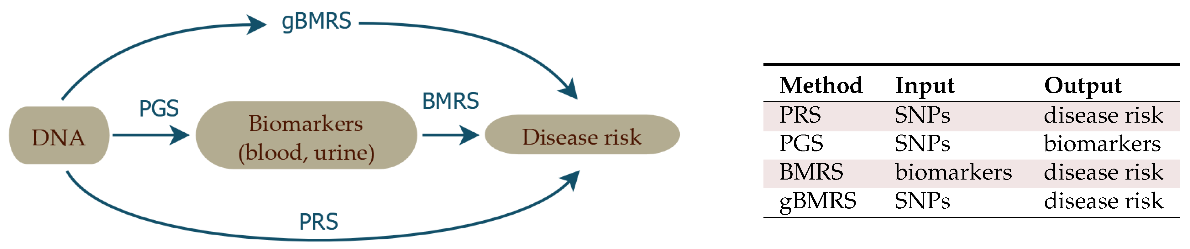
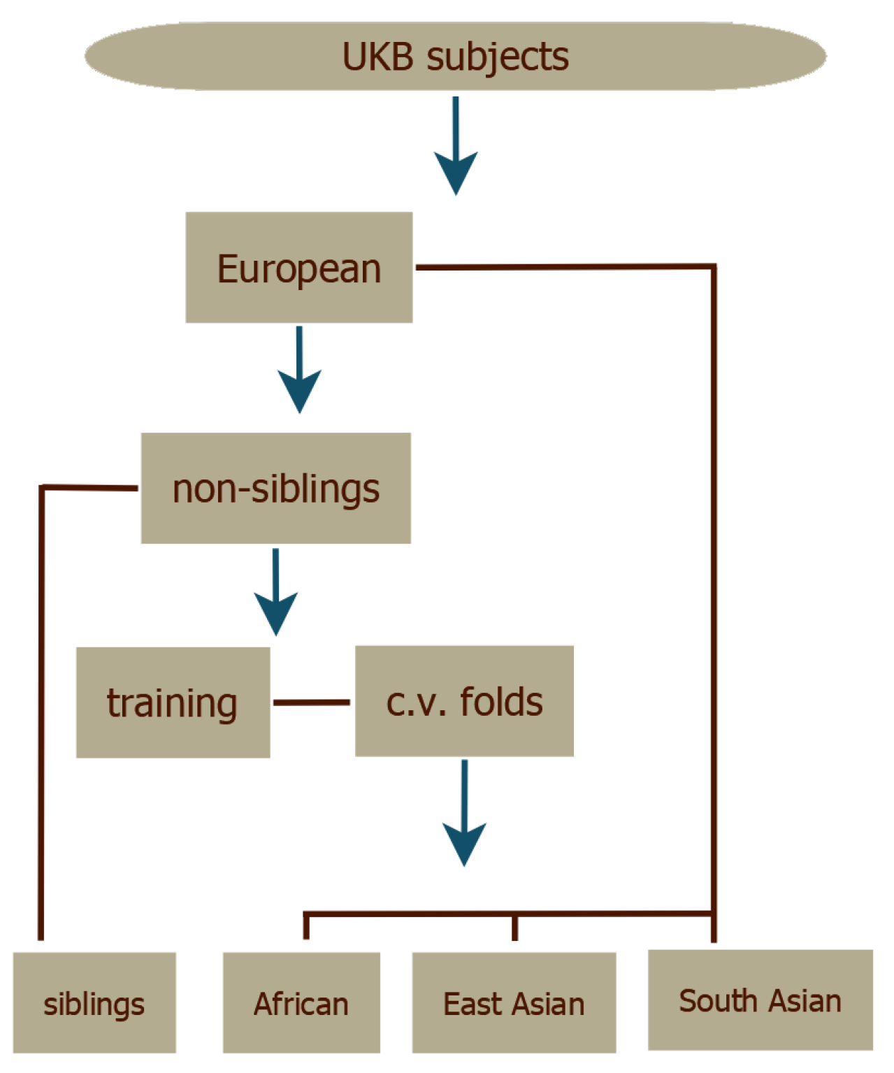
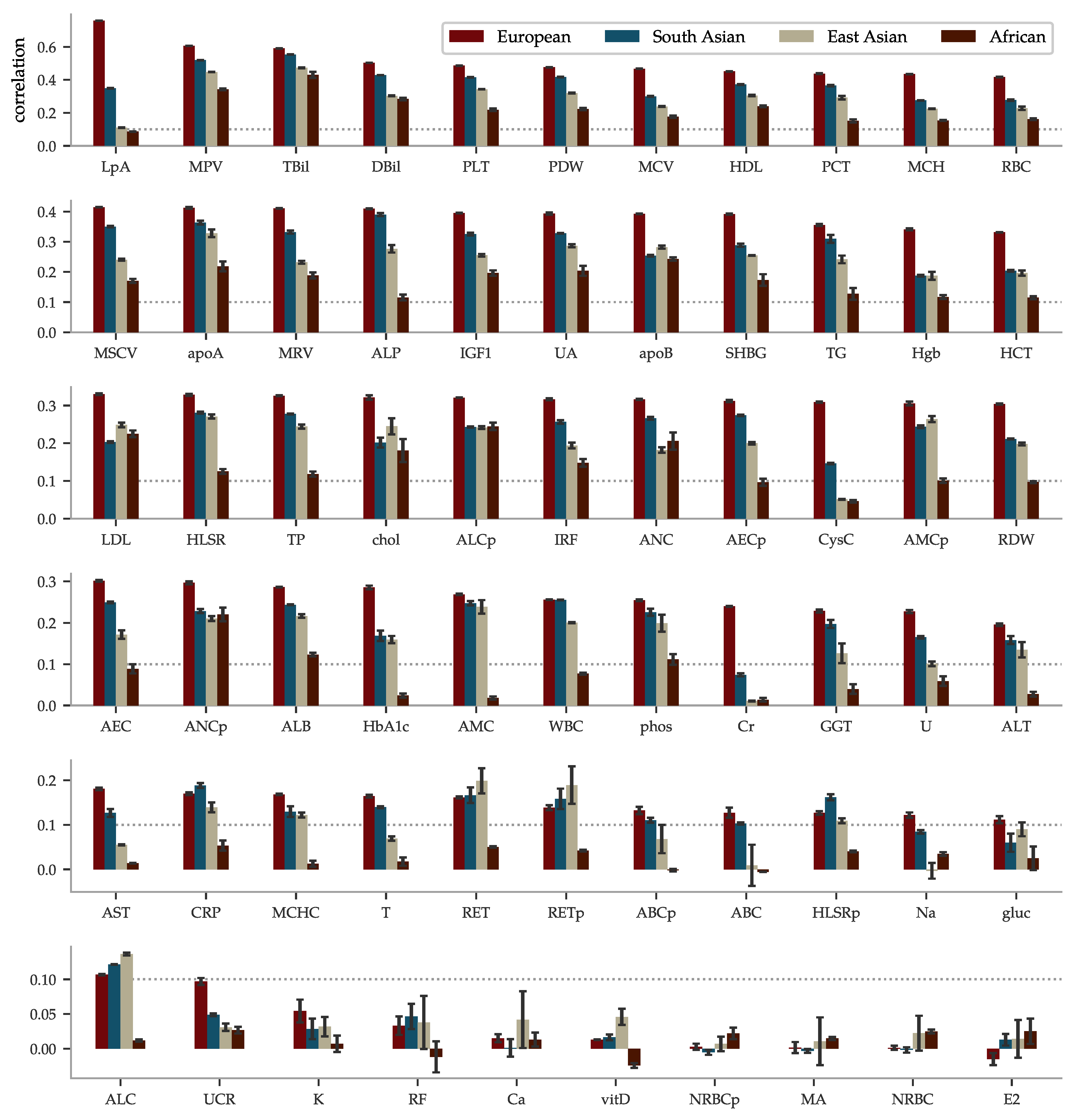
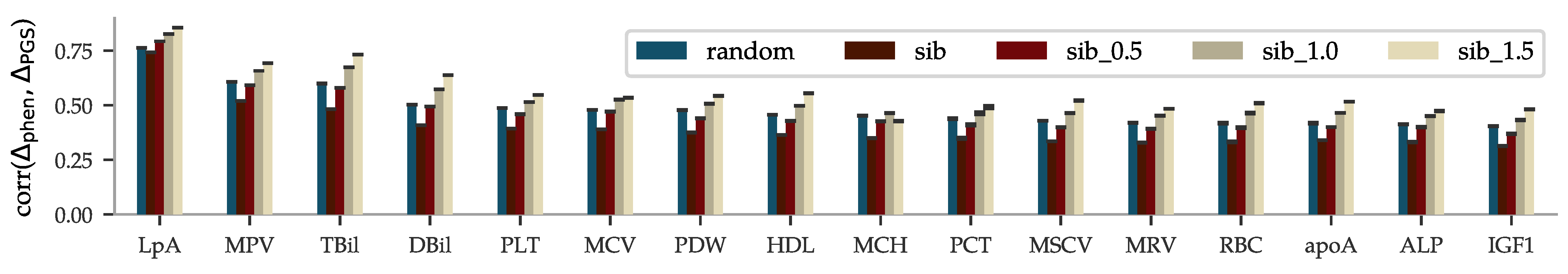
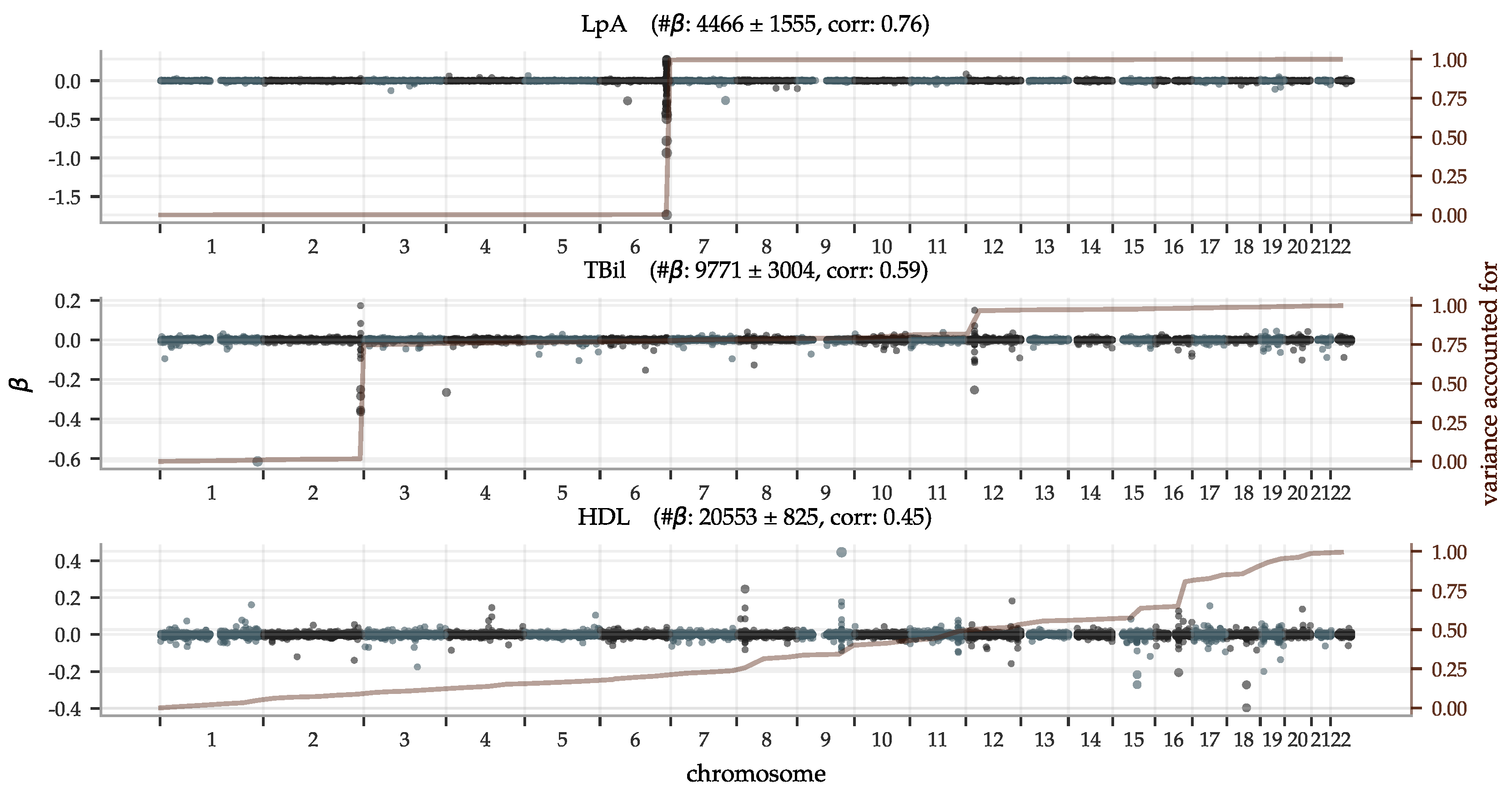
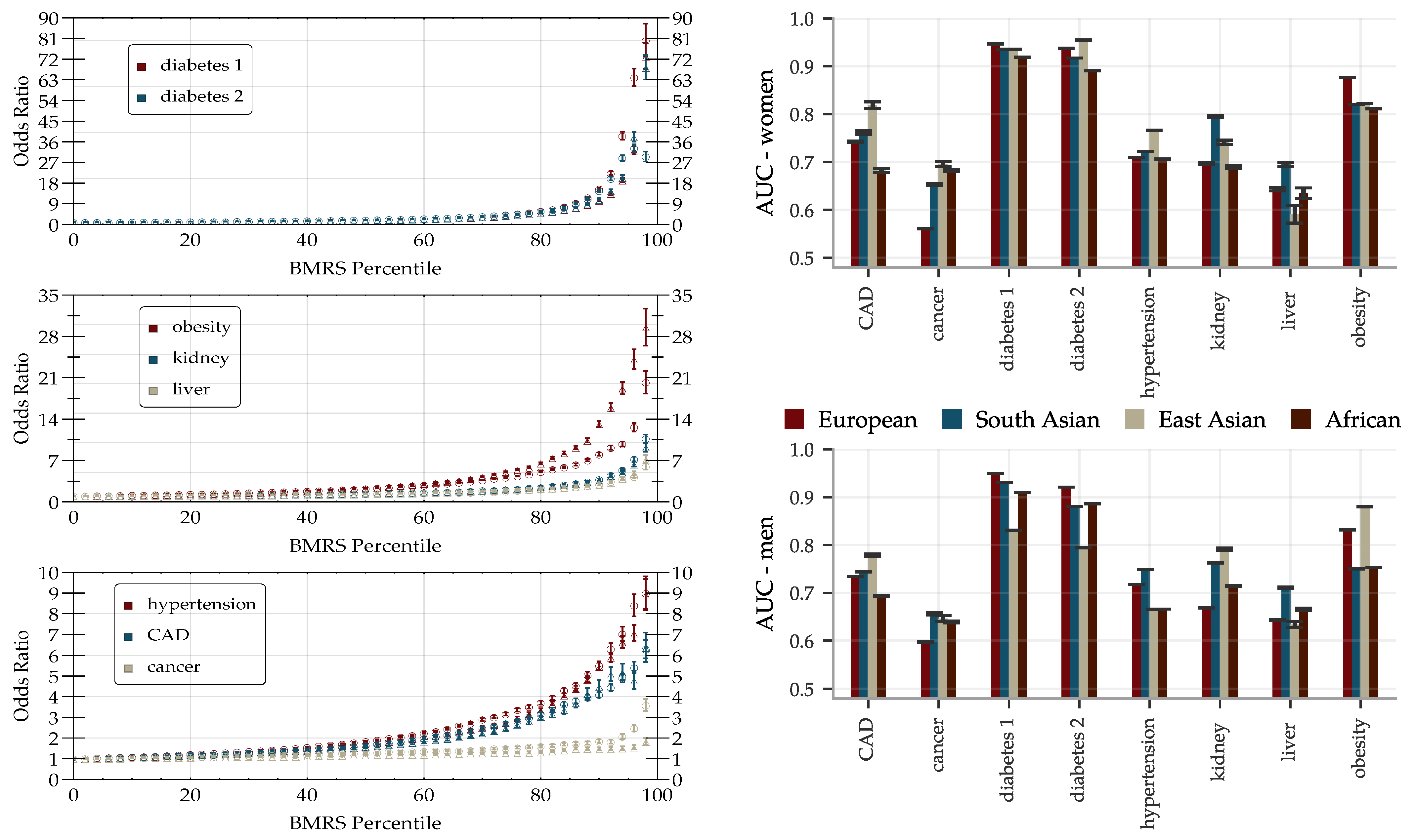
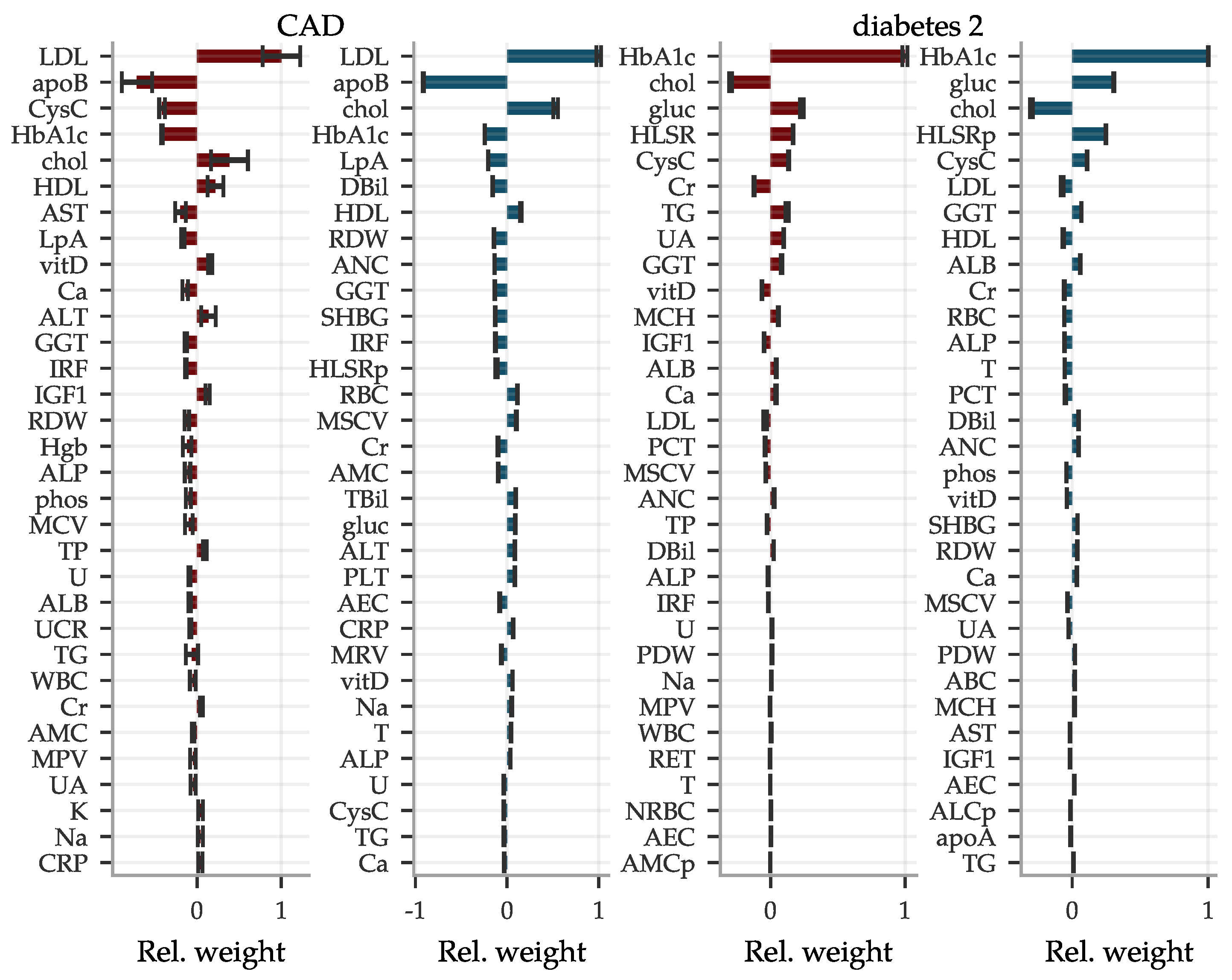
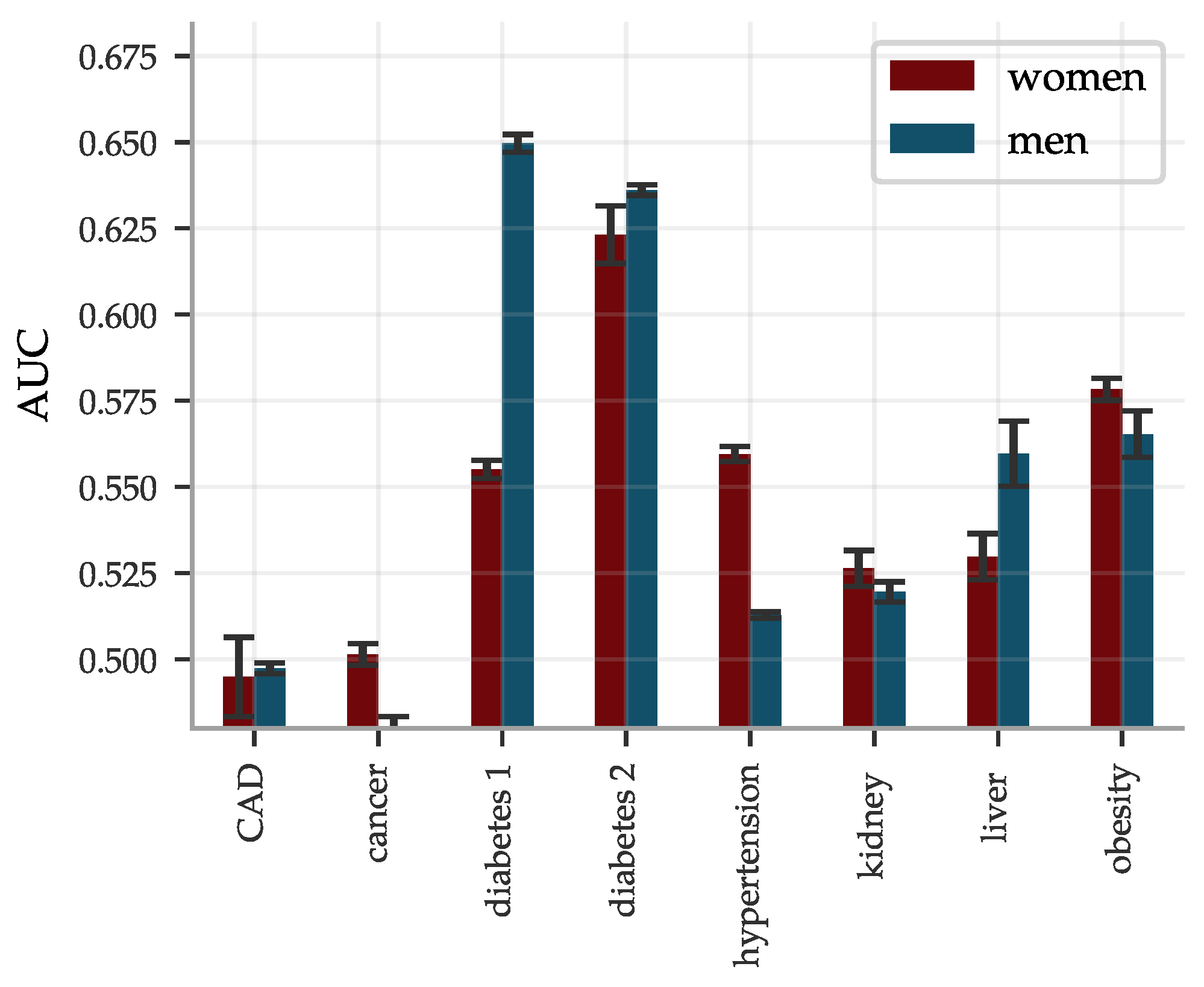
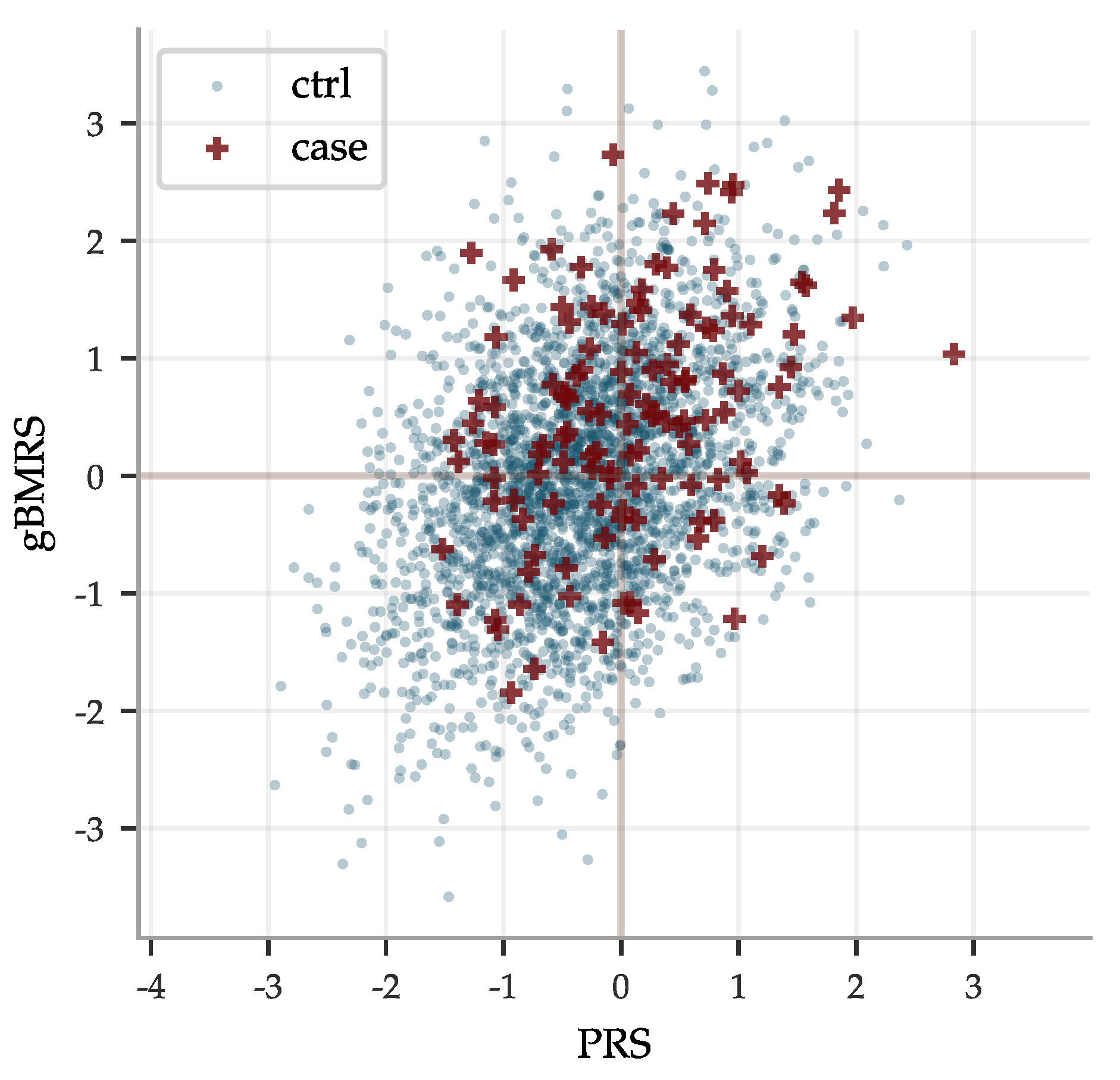
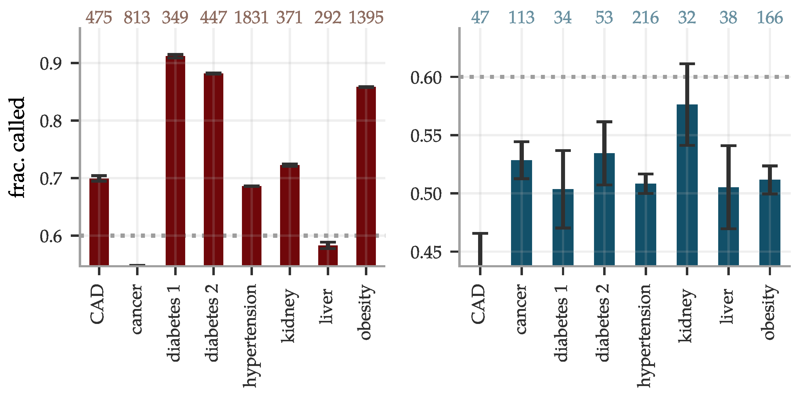
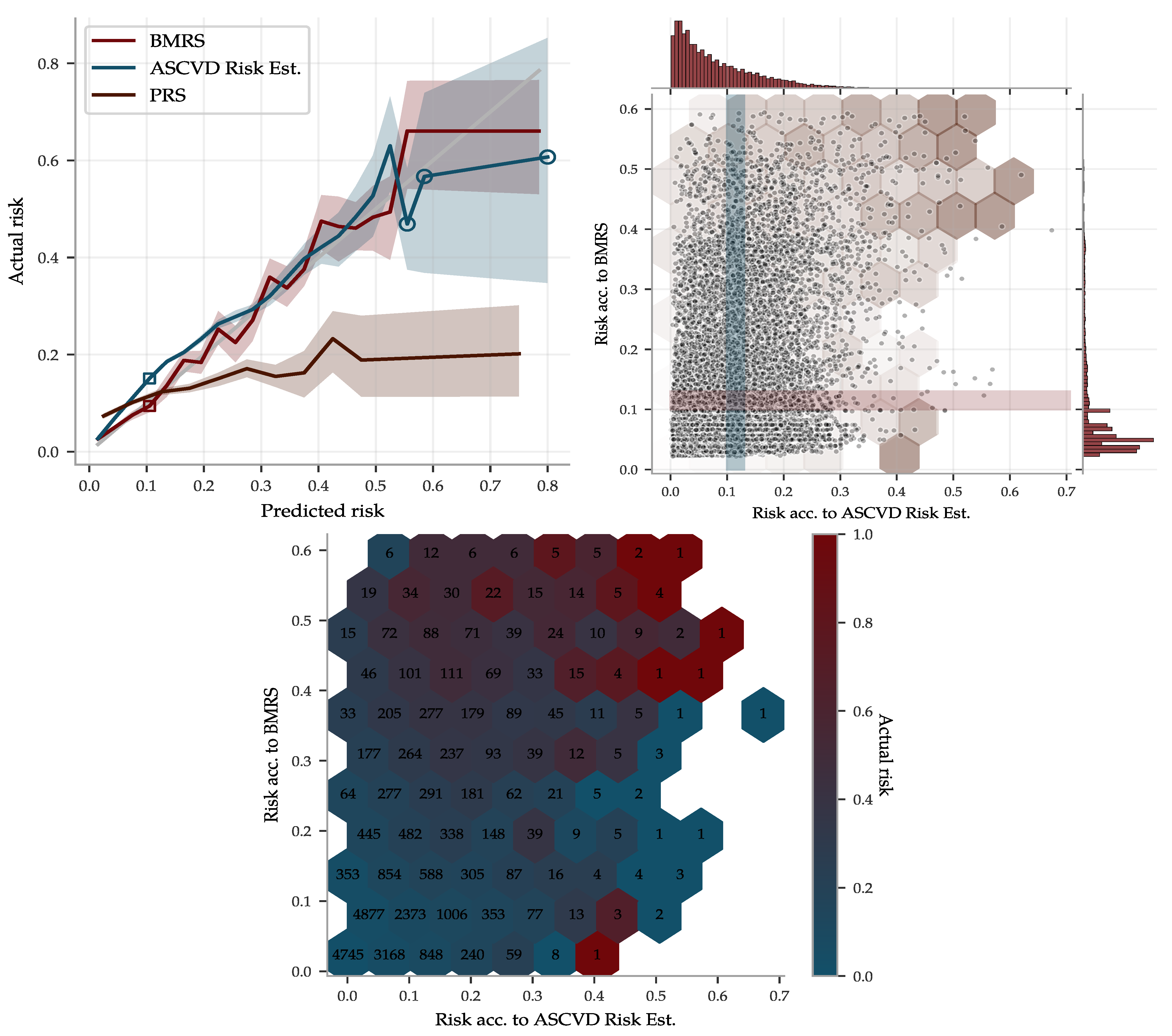
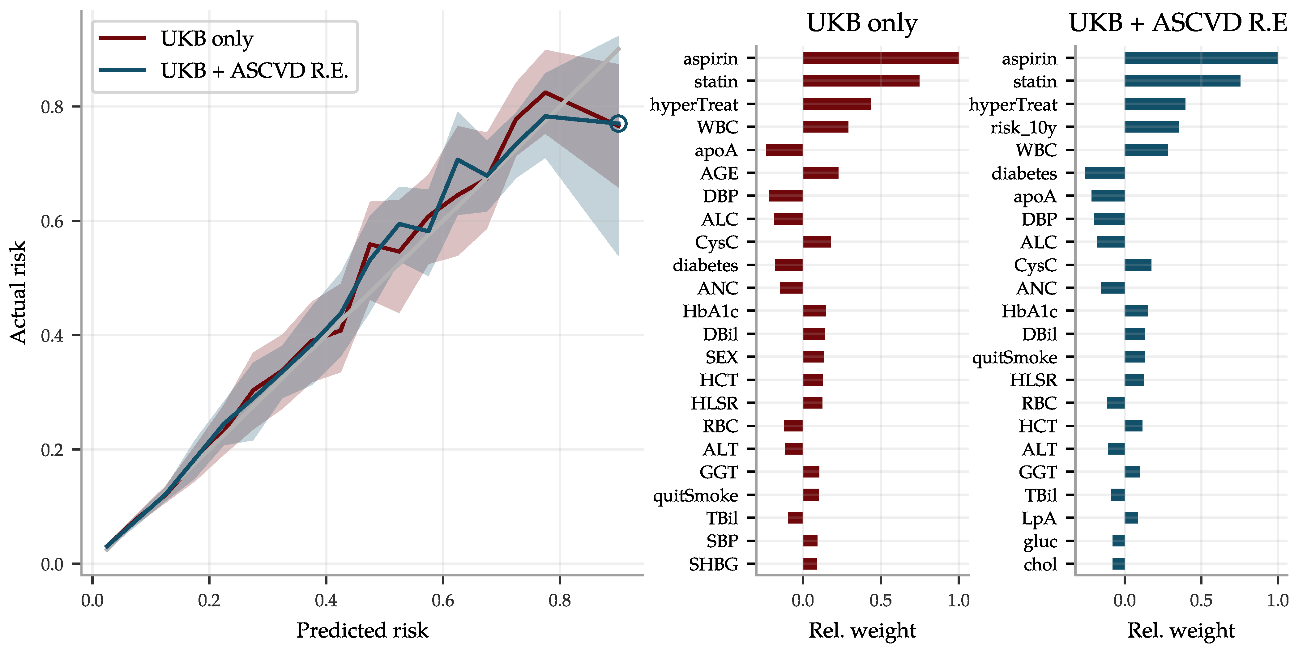
Table 1.
List of all studied blood and urine markers with abbreviations.
| Abbr. | Full Name | Abbr. | Full Name | Abbr. | Full Name |
|---|---|---|---|---|---|
| ABC | Basophill count | E2 | Oestradiol | NRBC | Nucleated red blood cell count |
| ABCp | Basophill percentage | GGT | Gamma glutamyltransferase | NRBCp | Nucleated red blood cell percentage |
| AEC | Eosinophill count | gluc | Glucose | PCT | Platelet crit |
| AECp | Eosinophill percentage | HbA1c | Glycated haemoglobin (HbA1c) | PDW | Platelet distribution width |
| ALB | Albumin | HCT | Haematocrit percentage | phos | Phosphate |
| ALC | Lymphocyte count | HDL | HDL cholesterol | PLT | Platelet count |
| ALCp | Lymphocyte percentage | Hgb | Haemoglobin concentration | RBC | Red blood cell (erythrocyte) count |
| ALP | Alkaline phosphatase | HLSR | High light scatter reticulocyte count | RDW | Red blood cell (erythrocyte) distribution width |
| ALT | Alanine aminotransferase | HLSRp | High light scatter reticulocyte percentage | RET | Reticulocyte count |
| AMC | Monocyte count | IGF1 | IGF-1 | RETp | Reticulocyte percentage |
| AMCp | Monocyte percentage | IRF | Immature reticulocyte fraction | RF | Rheumatoid factor |
| ANC | Neutrophill count | K | Potassium in urine | SHBG | SHBG |
| ANCp | Neutrophill percentage | LDL | LDL direct | T | Testosterone |
| apoA | Apolipoprotein A | LpA | Lipoprotein A | TBil | Total bilirubin |
| apoB | Apolipoprotein B | MA | Microalbumin in urine | TG | Triglycerides |
| AST | Aspartate aminotransferase | MCH | Mean corpuscular haemoglobin | TP | Total protein |
| Ca | Calcium | MCHC | Mean corpuscular haemoglobin concentration | U | Urea |
| chol | Cholesterol | MCV | Mean corpuscular volume | UA | Urate |
| Cr | Creatinine | MPV | Mean platelet (thrombocyte) volume | UCR | Creatinine (enzymatic) in urine |
| CRP | C-reactive protein | MRV | Mean reticulocyte volume | vitD | Vitamin D |
| CysC | Cystatin C | MSCV | Mean sphered cell volume | WBC | White blood cell (leukocyte) count |
| DBil | Direct bilirubin | Na | Sodium in urine |
Table 2.
Including Principal Component effect on the PGS predictors has negligible effect. Results are for self-reported Europeans within the sibling set.
Table 2.
Including Principal Component effect on the PGS predictors has negligible effect. Results are for self-reported Europeans within the sibling set.
| Abbr. | corr | corr ± std | corr ± std |
|---|---|---|---|
| HDL | 0.0128 | 0.4514 ± 0.0005 | 0.4574 ± 0.0002 |
| LpA | 0.0193 | 0.7591 ± 0.0003 | 0.7517 ± 0.0001 |
| TBil | 0.0338 | 0.5906 ± 0.0003 | 0.5838 ± 0.0001 |
| MCV | 0.0824 | 0.4673 ± 0.0004 | 0.4600 ± 0.0079 |
| MPV | 0.0290 | 0.6064 ± 0.0005 | 0.6061 ± 0.0008 |
Table 3.
Including Principal Component effect on the BMRS predictors has negligible impact on the AUCs. Shown is the relative AUC as computed in Equation (4) for self-reported Europeans within the sibling set, using the mean relative difference for 5 numbered predictors ± the standard deviation.
Table 3.
Including Principal Component effect on the BMRS predictors has negligible impact on the AUCs. Shown is the relative AUC as computed in Equation (4) for self-reported Europeans within the sibling set, using the mean relative difference for 5 numbered predictors ± the standard deviation.
| rel. AUC (women) | rel. AUC (men) | |
|---|---|---|
| CAD | 0.0027 ± 0.0160 | −0.0088 ± 0.0063 |
| cancer | −0.0060 ± 0.0089 | 0.0049 ± 0.0051 |
| diabetes 1 | −0.0068 ± 0.0026 | −0.0006 ± 0.0042 |
| diabetes 2 | −0.0002 ± 0.0037 | −0.0014 ± 0.0025 |
| hypertension | −0.0026 ± 0.0029 | 0.0005 ± 0.0024 |
| kidney | −0.0033 ± 0.0124 | −0.0074 ± 0.0161 |
| liver | −0.0108 ± 0.0113 | −0.0370 ± 0.0072 |
| obesity | −0.0004 ± 0.0011 | 0.0030 ± 0.0017 |
Publisher’s Note: MDPI stays neutral with regard to jurisdictional claims in published maps and institutional affiliations. |
© 2021 by the authors. Licensee MDPI, Basel, Switzerland. This article is an open access article distributed under the terms and conditions of the Creative Commons Attribution (CC BY) license (https://creativecommons.org/licenses/by/4.0/).
Share and Cite
MDPI and ACS Style
Widen, E.; Raben, T.G.; Lello, L.; Hsu, S.D.H. Machine Learning Prediction of Biomarkers from SNPs and of Disease Risk from Biomarkers in the UK Biobank. Genes 2021, 12, 991. https://0-doi-org.brum.beds.ac.uk/10.3390/genes12070991
AMA Style
Widen E, Raben TG, Lello L, Hsu SDH. Machine Learning Prediction of Biomarkers from SNPs and of Disease Risk from Biomarkers in the UK Biobank. Genes. 2021; 12(7):991. https://0-doi-org.brum.beds.ac.uk/10.3390/genes12070991
Chicago/Turabian StyleWiden, Erik, Timothy G. Raben, Louis Lello, and Stephen D. H. Hsu. 2021. "Machine Learning Prediction of Biomarkers from SNPs and of Disease Risk from Biomarkers in the UK Biobank" Genes 12, no. 7: 991. https://0-doi-org.brum.beds.ac.uk/10.3390/genes12070991
Note that from the first issue of 2016, this journal uses article numbers instead of page numbers. See further details here.