On the Impact of Trees on Ventilation in a Real Street in Pamplona, Spain

 ,
,  , ,
, ,  and
and
Abstract
:1. Introduction
- -
- Aerodynamic effects, i.e., trees modify the wind flow around them changing the distribution of pollutants.
- -
- Deposition effects, i.e., a fraction of pollutant is removed from the air by means of pollutant deposition on tree leaves and absorption through stomata.
2. Methodology
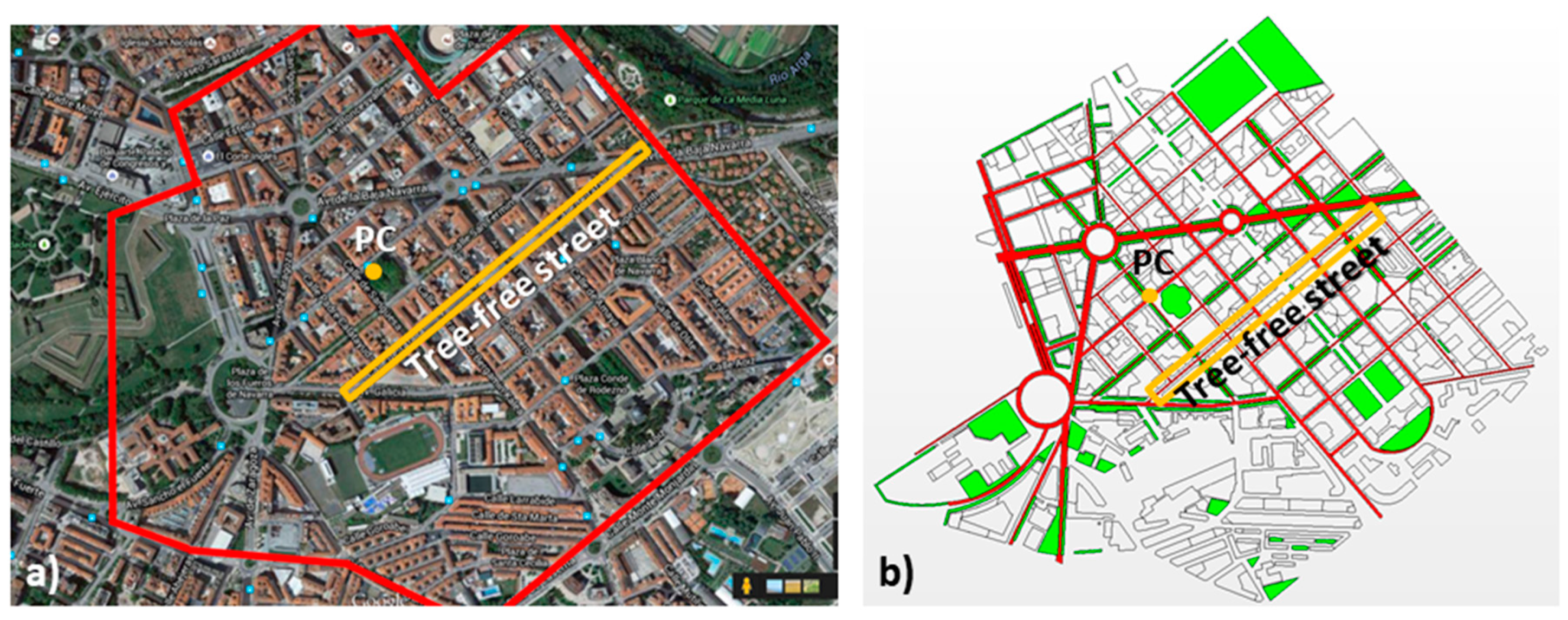
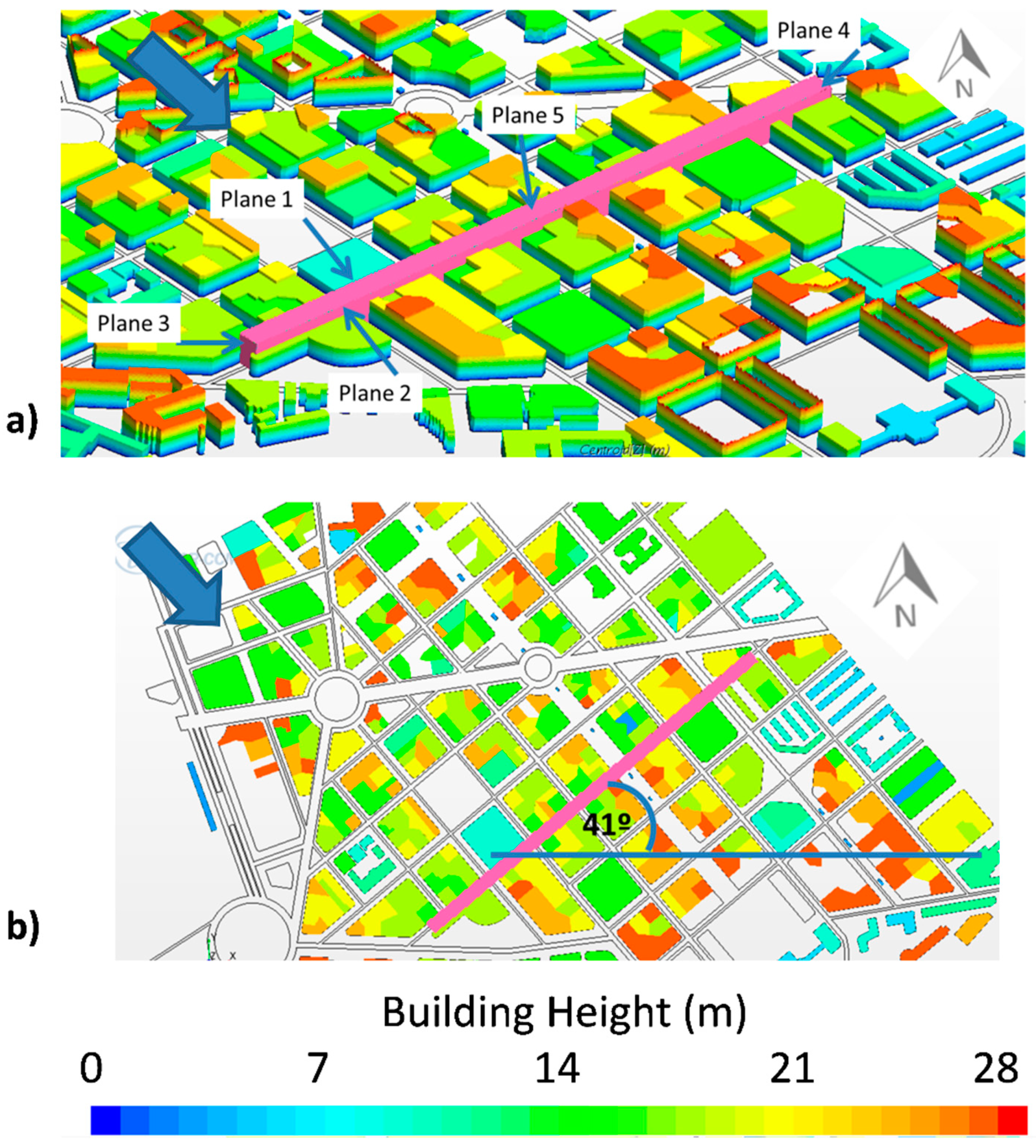
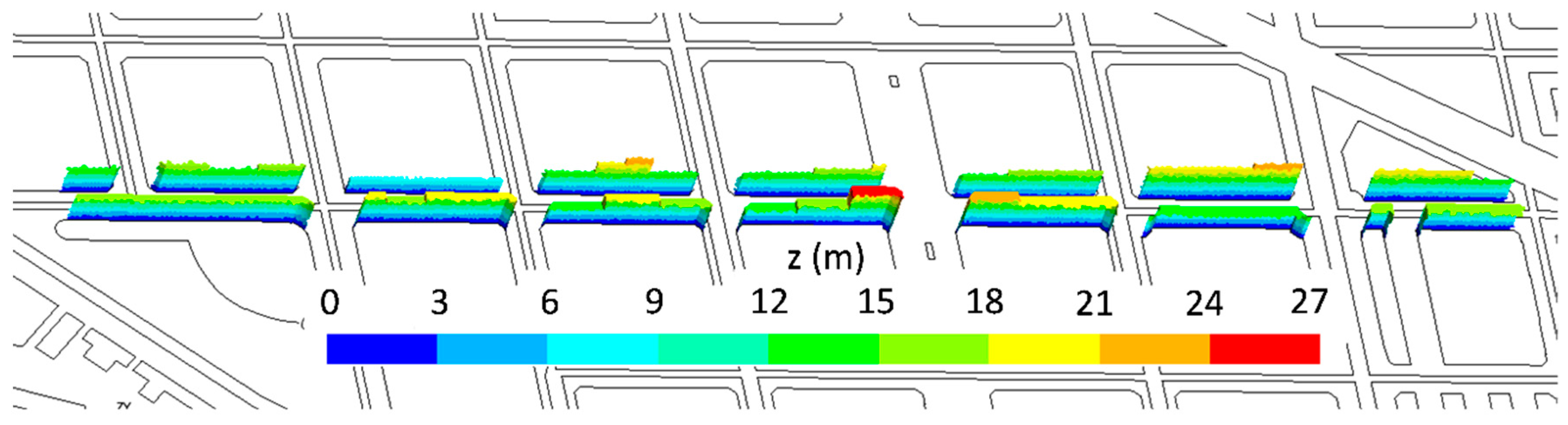
2.1. The Study Area
2.2. Summary of the Previous Analysis
2.3. Extension of the Analysis to Flow, Turbulence and Ventilation
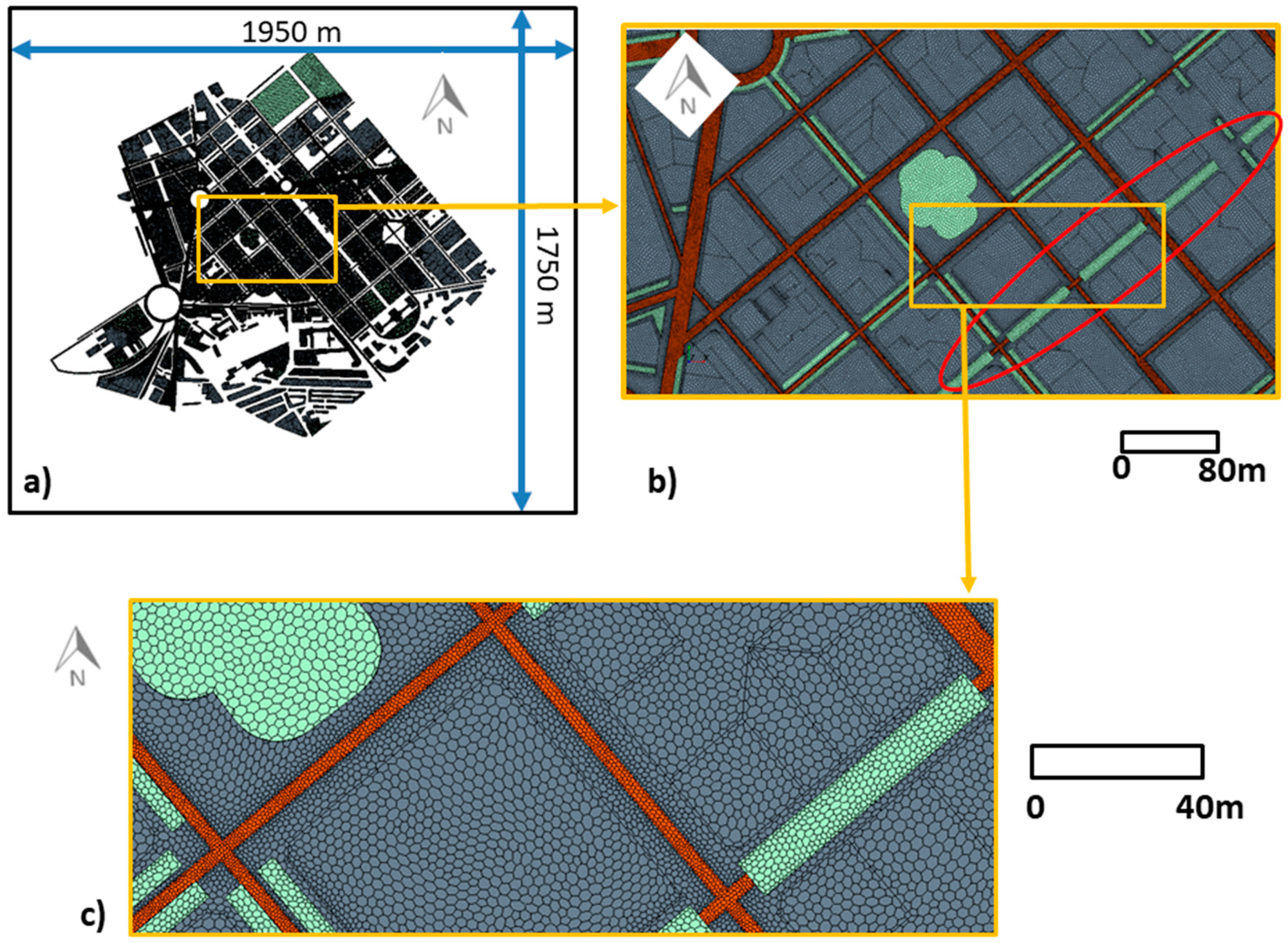
3. CFD Simulation Setup
Evaluation of the Modeling Approach Used in the Present Study
4. Results
4.1. Spatially-Averaged Concentration over the Whole Neighborhood
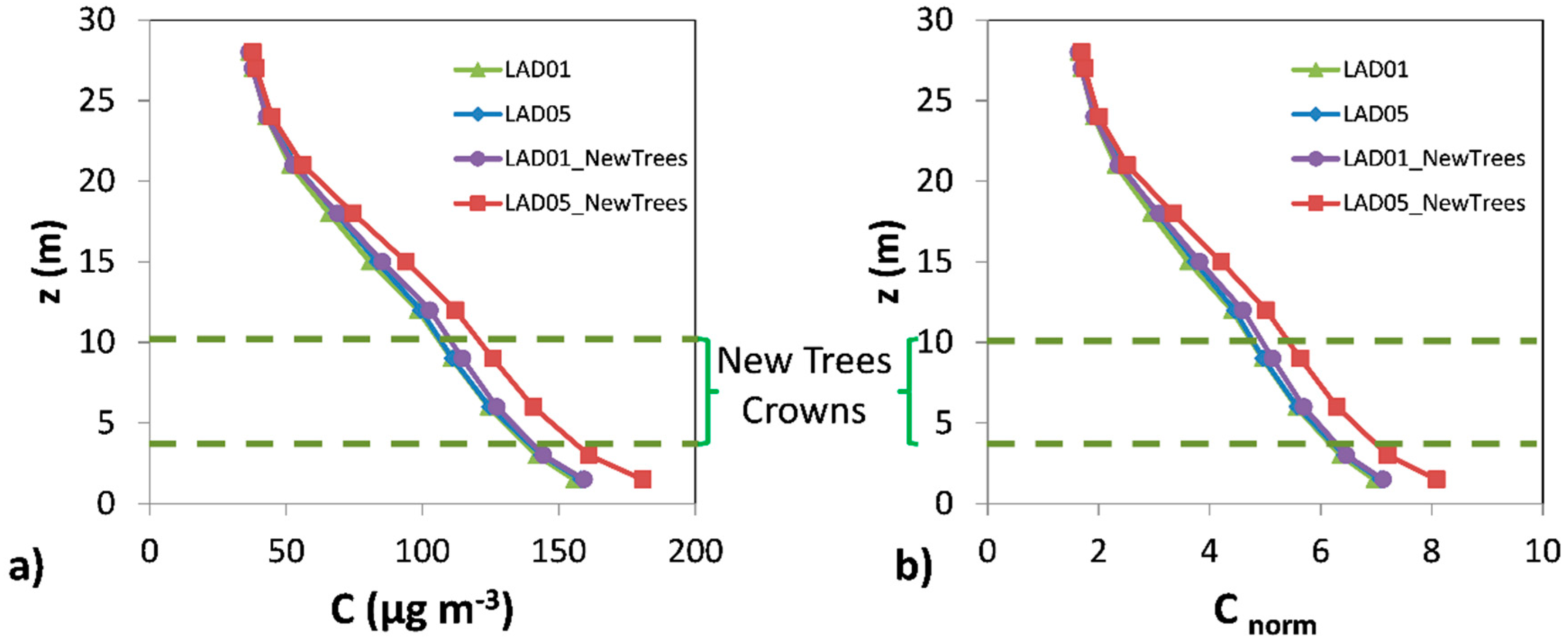
4.2. Spatially-Averaged Concentration in the Tafalla Street
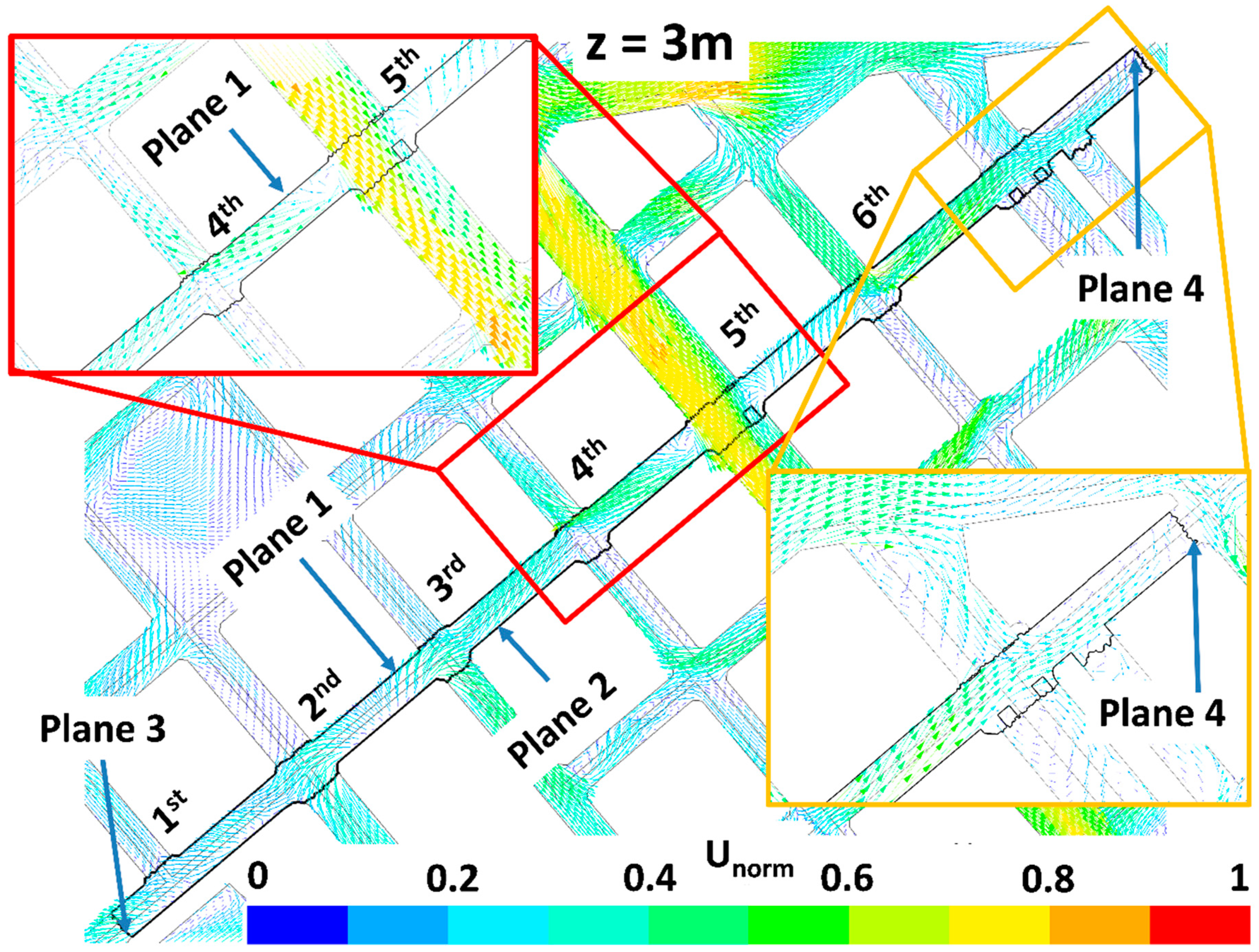
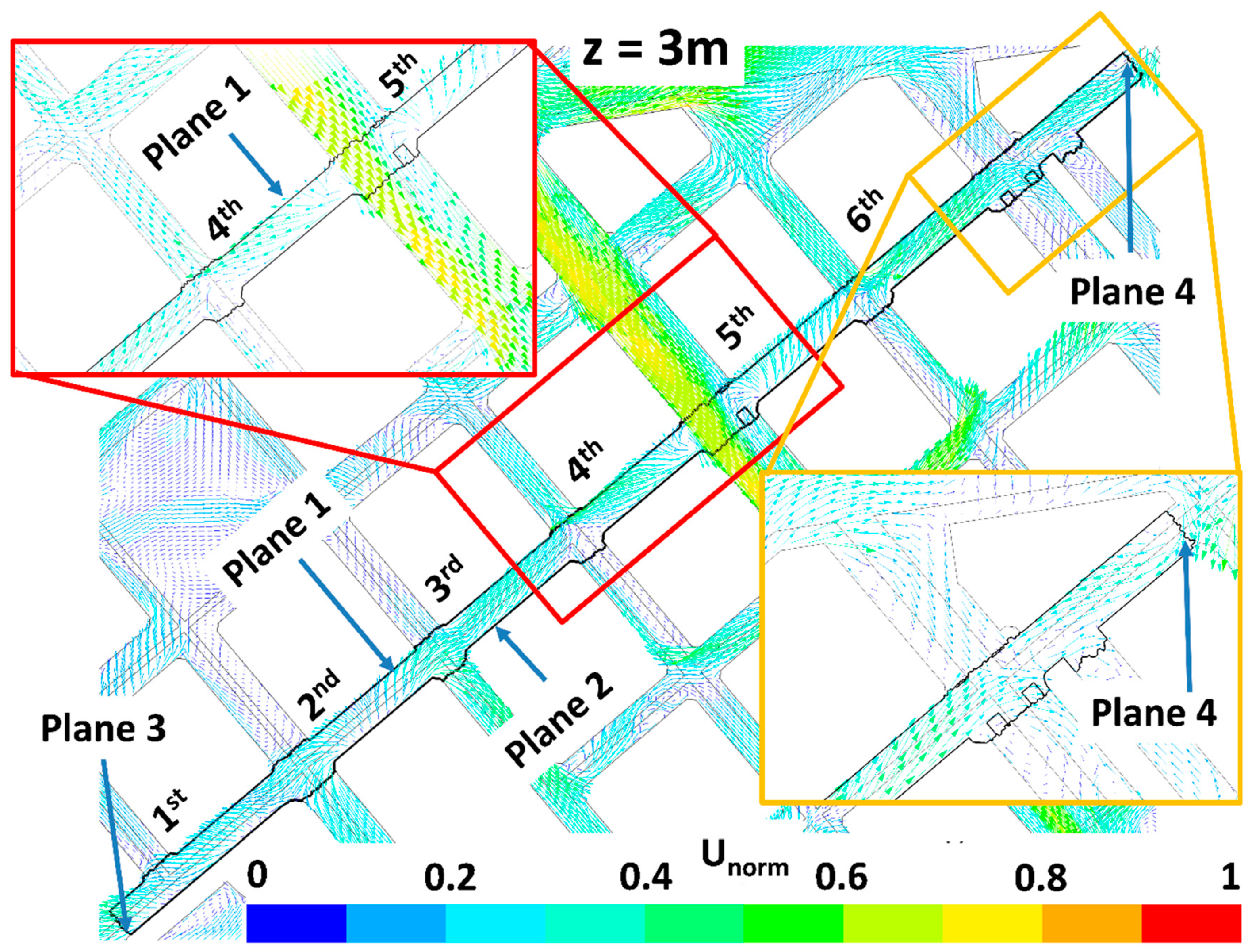
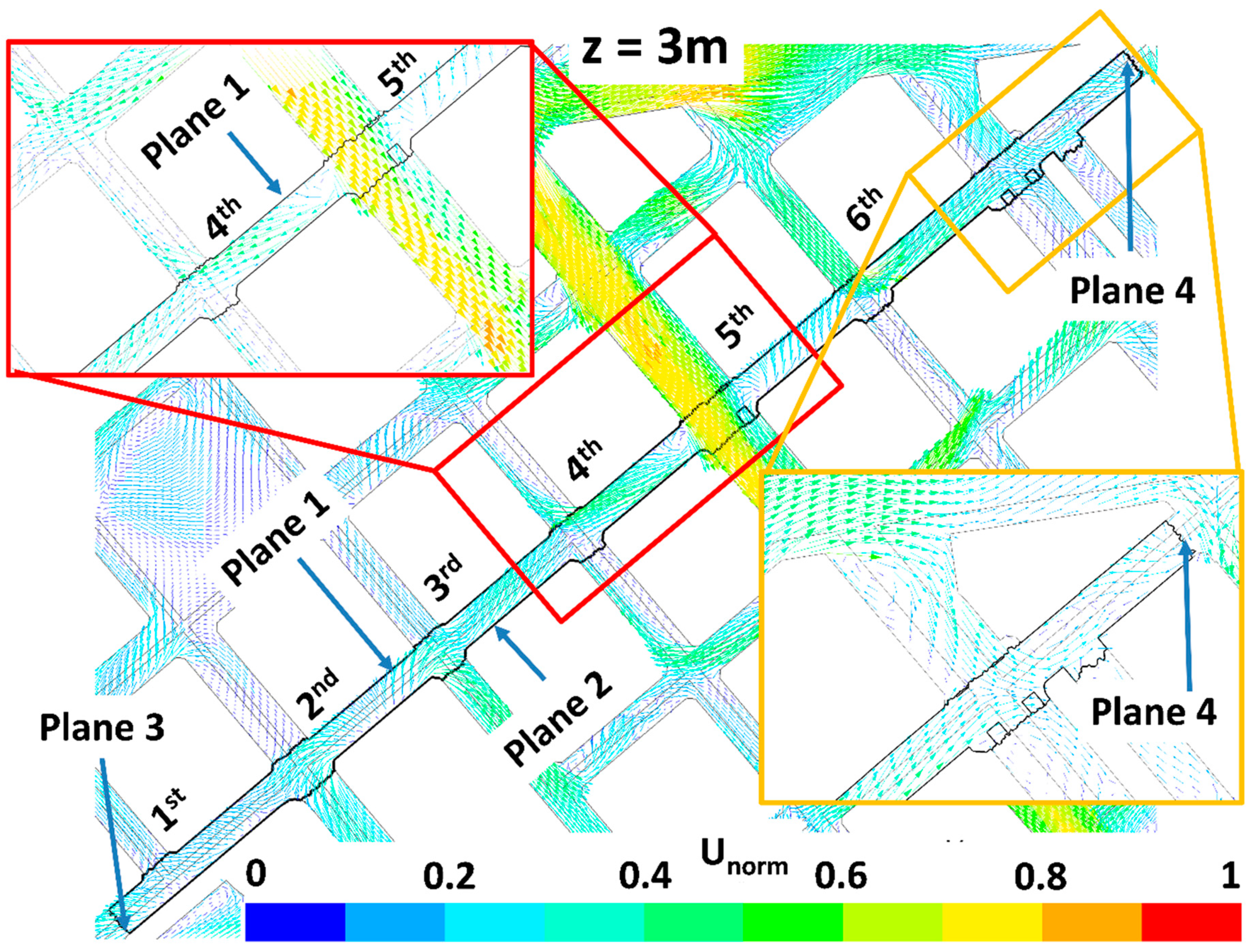
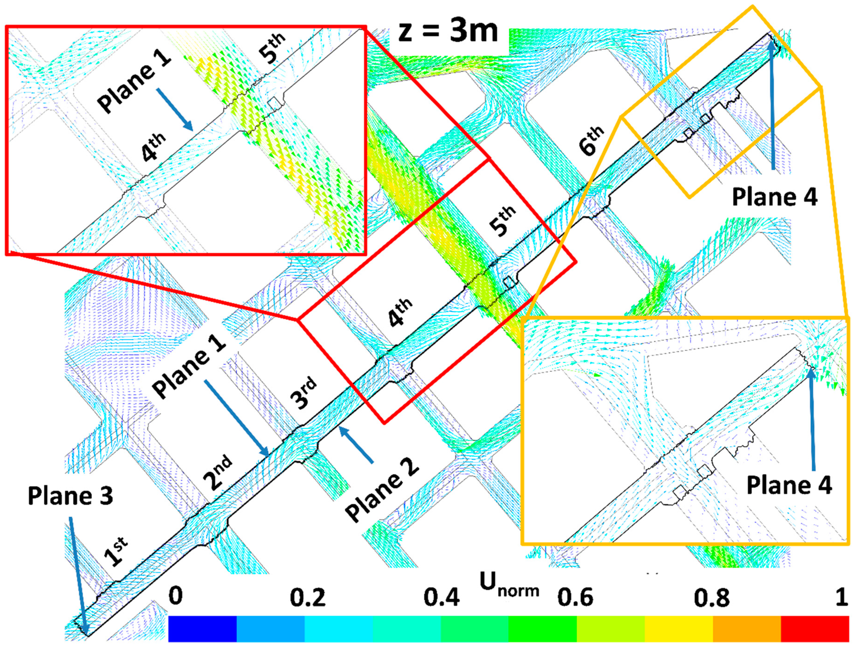
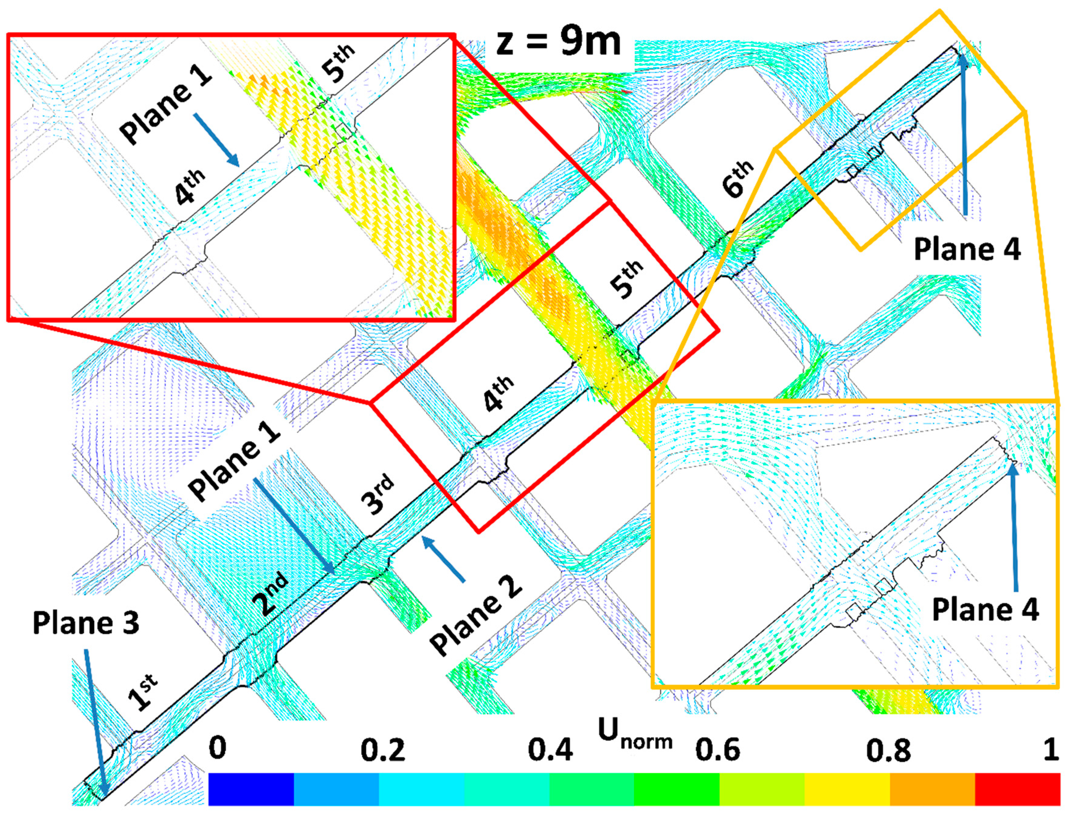
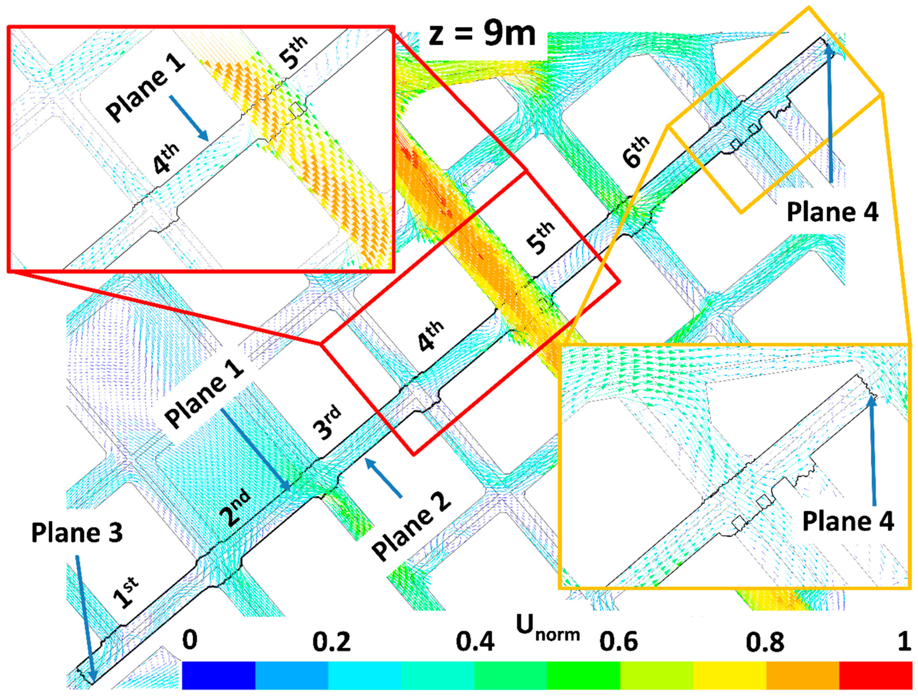
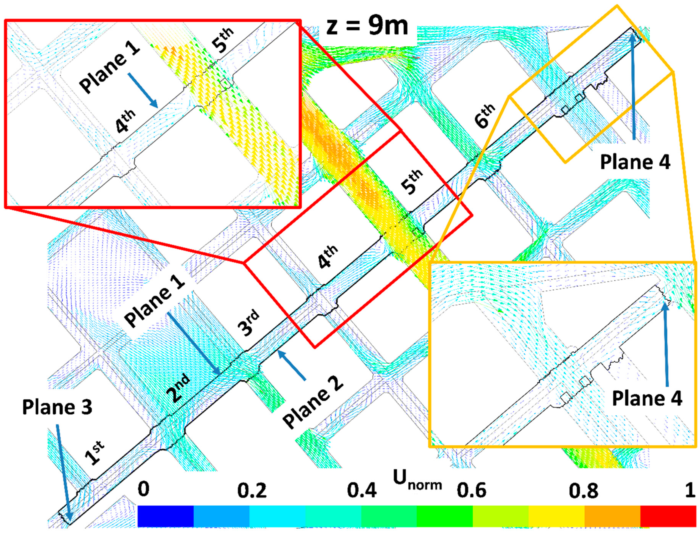
4.3. Wind Flow Patterns and Ventilation in Tafalla Street
5. Conclusions
- The increase of total pollutant mass flow rates entering the street;
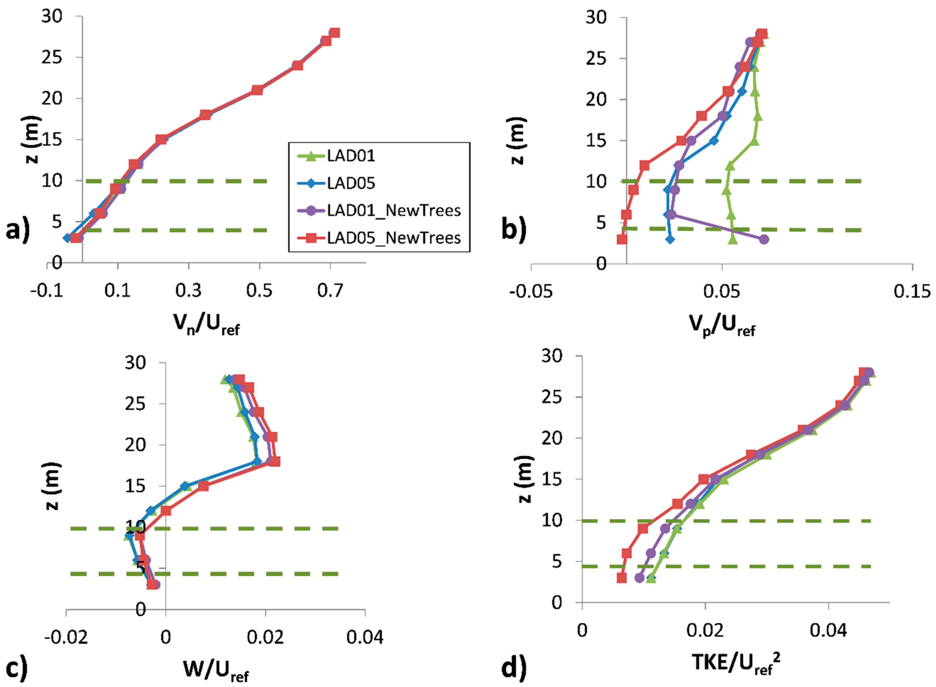
- The change of the ventilation. In fact, the average wind speed parallel to the street (parallel ventilation) and the downward vertical wind speed within the new vegetation canopy were reduced with respect to tree-free street scenarios. This fact implied a weaker ventilation within and below the vegetation canopy. Further, the turbulent kinetic energy decreased within and below the new vegetation canopy, and consequently reduced the pollutant dispersion.
Author Contributions
Funding
Acknowledgments
Conflicts of Interest
References
- Weissert, L.F.; Salmond, J.A.; Schwendenmann, L. A review of the current progress in quantifying the potential of urban forests to mitigate urban CO2 emissions. Urban Clim. 2014, 8, 100–125. [Google Scholar] [CrossRef]
- Salmond, J.A.; Tadaki, M.; Vardoulakis, S.; Arbuthnott, K.; Coutts, A.; Demuzere, M.; Dirks, K.N.; Heaviside, C.; Lim, S.; Macintyre, H.; et al. Health and climate related ecosystem services provided by street trees in the urban environment. Environ. Health 2016, 15, 95–111. [Google Scholar] [CrossRef] [PubMed]
- Santamouris, M.; Ban-Weiss, G.; Osmond, P.; Paolini, R.; Synnefa, A.; Cartalis, C.; Muscio, A.; Zinzi, M.; Morakinyo, T.; Ng, E.; et al. Progress in urban greenery mitigation science—Assessment methodologies advanced technologies and impact on cities. J. Civ. Eng. Manag. 2018, 24, 638–671. [Google Scholar] [CrossRef]
- Escobedo, F.J.; Giannico, V.; Jim, C.Y.; Sanesi, G.; Lafortezza, R. Urban forests, ecosystem services, green infrastructure and nature-based solutions: Nexus or evolving metaphors? Urban For. Urban Green. 2019, 37, 3–12. [Google Scholar] [CrossRef]
- Renterghem, T.V. Towards explaining the positive effect of vegetation on the perception of environmental noise. Urban For. Urban Green. 2019, 40, 133–144. [Google Scholar] [CrossRef]
- Pearlmutter, D.; Calfapietra, C.; Samson, R.; O’Brien, L.; Krajter Ostoic, S.; Sanesi, G.; Alonso del Amo, R. The Urban Forest: Cultivating Green Infrastructure for People and the Environment; Future City 7; Springer: Berlin, Germany, 2017; ISBN 978-3-319-50279-3. [Google Scholar]
- Janhäll, S. Review on urban vegetation and particle air pollution—Deposition and dispersion. Atmos. Environ. 2015, 105, 130–137. [Google Scholar] [CrossRef]
- Ramponi, R.; Blocken, B.; de Coo, L.B.; Janssen, W.D. CFD simulation of outdoor ventilation of generic urban configurations with different urban densities and equal and unequal street widths. Build. Environ. 2015, 92, 152–166. [Google Scholar] [CrossRef]
- Buccolieri, R.; Hang, J. Recent advances in urban ventilation assessment and flow modelling. Atmosphere 2019, 10, 144. [Google Scholar] [CrossRef]
- Abhijith, K.V.; Kumar, P.; Gallagher, J.; McNabola, A.; Baldauf, R.; Pilla, F.; Broderick, B.; Di Sabatino, S.; Pulvirenti, B. Air pollution abatement performances of green infrastructure in open road and built-up street canyon environments—A review. Atmos. Environ. 2017, 162, 71–86. [Google Scholar] [CrossRef]
- Buccolieri, R.; Santiago, J.L.; Rivas, E.; Sanchez, B. Review on urban tree modelling in CFD simulations: Aerodynamic, deposition and thermal effects. Urban For. Urban Green. 2018, 31, 212–220. [Google Scholar] [CrossRef]
- Gallagher, J.; Baldauf, R.; Fuller, C.H.; Kumar, P.; Gill, L.W.; McNabola, A. Passive methods for improving air quality in the built environment: A review of porous and solid barriers. Atmos. Environ. 2015, 120, 61–70. [Google Scholar] [CrossRef]
- Santiago, J.-L.; Buccolieri, R.; Rivas, E.; Calvete-Sogo, H.; Sanchez, B.; Martilli, A.; Alonso, R.; Elustondo, D.; Santamaría, J.M.; Martin, F. CFD modelling of vegetation barrier effects on the reduction of traffic-related pollutant concentration in an avenue of Pamplona, Spain. Sustain. Cities Soc. 2019, 48, 101559. [Google Scholar] [CrossRef]
- Vos, P.E.; Maiheu, B.; Vankerkom, J.; Janssen, S. Improving local air quality in cities: To tree or not to tree? Environ. Pollut. 2013, 183, 113–122. [Google Scholar] [CrossRef] [PubMed]
- Gromke, C.; Blocken, B. Influence of avenue-trees on air quality at the urban neighborhood scale. Part II: Traffic pollutant concentrations at pedestrian level. Environ. Pollut. 2015, 196, 176–184. [Google Scholar] [CrossRef] [PubMed]
- Santiago, J.-L.; Martilli, A.; Martin, F. On Dry Deposition Modelling of Atmospheric Pollutants on Vegetation at the Microscale: Application to the Impact of Street Vegetation on Air Quality. Bound.-Layer Meteorol. 2017, 162, 451–474. [Google Scholar] [CrossRef]
- Jeanjean, A.P.; Monks, P.S.; Leigh, R.J. Modelling the effectiveness of urban trees and grass on PM2.5 reduction via dispersion and deposition at a city scale. Atmos. Environ. 2016, 147, 1–10. [Google Scholar] [CrossRef]
- Jeanjean, A.P.; Buccolieri, R.; Eddy, J.; Monks, P.S.; Leigh, R.J. Air quality affected by trees in real street canyons: The case of Marylebone neighbourhood in central London. Urban For. Urban Green. 2017, 22, 41–53. [Google Scholar] [CrossRef]
- Buccolieri, R.; Jeanjean, A.P.R.; Gatto, E.; Leigh, R.J. The impact of trees on street ventilation, NOx and PM2.5 concentrations across heights in Marylebone Rd street canyon, central London. Sustain. Cities Soc. 2018, 41, 227–241. [Google Scholar] [CrossRef]
- Santiago, J.L.; Rivas, E.; Sanchez, B.; Buccolieri, R.; Martin, F. The impact of planting trees on NOx concentrations: The case of the Plaza de la Cruz neighborhood in Pamplona (Spain). Atmosphere 2017, 8, 131. [Google Scholar] [CrossRef]
- Buccolieri, R.; Sandberg, M.; Di Sabatino, S. City breathability and its link to pollutant concentration distribution within urban-like geometries. Atmos Environ. 2010, 44, 1894–1903. [Google Scholar]
- Hang, J.; Li, Y.; Buccolieri, R.; Sandberg, M.; Di Sabatino, S. On the contribution of mean flow and turbulence to city breathability: The case of long streets with tall buildings. Sci. Total Environ. 2012, 416, 362–373. [Google Scholar] [CrossRef] [PubMed]
- Rivas, E.; Santiago, J.L.; Lechón, Y.; Martín, F.; Ariño, A.; Pons, J.J.; Santamaría, J.M. CFD modelling of air quality in Pamplona City (Spain): Assessment, stations spatial representativeness and health impacts valuation. Sci. Total Environ. 2019, 649, 1362–1380. [Google Scholar] [CrossRef] [PubMed]
- Sanz, C. A note on k − ε modeling of vegetation canopy air-flows. Bound.-Layer Meteorol. 2003, 108, 191–197. [Google Scholar] [CrossRef]
- Franke, J.; Schlünzen, H.; Carissimo, B. Best Practice Guideline for the CFD Simulation of Flows in the Urban Environment. In COST Action 732—Quality Assurance and Improvement of Microscale Meteorological Models; University of Hamburg (Germany), Meteorological Institute: Hamburg, Germany, 2007; ISBN 3-00-018312-4. [Google Scholar]
- Di Sabatino, S.; Buccolieri, R.; Olesen, H.R.; Ketzel, M.; Berkowicz, R.; Franke, J.; Schatzmann, M.; Schlunzen, K.; Leitl, B.; Britter, R.; et al. COST 732 in practice: The MUST model evaluation exercise. International. J. Environ. Pollut. 2011, 44, 403–418. [Google Scholar] [CrossRef]
- Richards, P.J.; Hoxey, R.P. Appropriate boundary conditions for computational wind engineering models using the k-ϵ turbulence model. J. Wind Eng. Ind. Aerodyn. 1993, 46, 145–153. [Google Scholar] [CrossRef]
- Buccolieri, R.; Salim, S.M.; Leo, L.S.; Di Sabatino, S.; Chan, A.; Ielpo, P.; Gromke, C. Analysis of local scale tree–atmosphere interaction on pollutant concentration in idealized street canyons and application to a real urban junction. Atmos. Environ. 2011, 45, 1702–1713. [Google Scholar] [CrossRef]
- Santiago, J.L.; Martín, F.; Martilli, A. A computational fluid dynamic modelling approach to assess the representativeness of urban monitoring stations. Sci. Total Environ. 2013, 454–455, 61–72. [Google Scholar] [CrossRef] [PubMed]
- Santiago, J.L.; Borge, R.; Martin, F.; de la Paz, D.; Martilli, A.; Lumbreras, J.; Sanchez, B. Evaluation of a CFD-based approach to estimate pollutant distribution within a real urban canopy by means of passive samplers. Sci. Total Environ. 2017, 576, 46–58. [Google Scholar] [CrossRef] [PubMed]
- Krayenhoff, E.S.; Santiago, J.L.; Martilli, A.; Christen, A.; Oke, T.R. Parametrization of drag and turbulence for urban neighbourhoods with trees. Bound.-Layer Meteorol. 2015, 156, 157–189. [Google Scholar] [CrossRef]
- Brunet, Y.; Finnigan, J.J.; Raupach, M.R. A wind tunnel study of air flow in waving wheat: Single-point velocity statistics. Bound.-Layer Meteorol. 1994, 70, 95–132. [Google Scholar] [CrossRef]
- Raupach, M.R.; Bradley, E.F.; Ghadiri, H. Wind Tunnel Investigation into the Aerodynamic Effect of Forest Clearing on the Nesting of Abbott’s Booby on Christmas Island; Internal Report; CSIRO Centre for Environmental Mechanics: Canberra, Australia, 1987. [Google Scholar]
- Foudhil, H.; Brunet, Y.; Caltagirone, J.P. A Fine-Scale k−ε Model for Atmospheric Flow over Heterogeneous Landscapes. Environ. Fluid Mech. 2005, 5, 247–265. [Google Scholar] [CrossRef]
- Dupont, S.; Brunet, Y. Edge flow and canopy structure: A large-eddy simulation study. Bound.-Layer Meteorol. 2008, 126, 51–71. [Google Scholar] [CrossRef]
- Gromke, C.; Ruck, B. Influence of trees on the dispersion of pollutants in an urban street canyon-experimental investigation of the flow and concentration field. Atmos. Environ. 2007, 41, 3287–3302. [Google Scholar] [CrossRef] [Green Version]
- Gromke, C.; Ruck, B. On the impact of trees on dispersion processes of traffic emissions in street canyons. Bound.-Layer Meteorol. 2009, 131, 19–34. [Google Scholar] [CrossRef]
- Gromke, C.; Buccolieri, R.; Di Sabatino, S.; Ruck, B. Dispersion study in a street canyon with tree planting by means of wind tunnel and numerical investigations—Evaluation of CFD data with experimental data. Atmos. Environ. 2008, 42, 8640–8650. [Google Scholar] [CrossRef]
- Balczó, M.; Gromke, C.; Ruck, B. Numerical modeling of flow and pollutant dispersion in street canyons with tree planting. Meteorol. Z. 2009, 18, 197–206. [Google Scholar] [CrossRef]
- Vranckx, S.; Vos, P.; Maiheu, B.; Janssen, S. Impact of trees on pollutant dispersion in street canyons: A numerical study of the annual average effects in Antwerp, Belgium. Sci. Total Environ. 2015, 532, 474–483. [Google Scholar] [CrossRef] [PubMed]
- Moonen, P.; Gromke, C.; Dorer, V. Performance assessment of large eddy simulation (LES) for modelling dispersion in an urban street canyon with tree planting. Atmos. Environ. 2013, 75, 66–76. [Google Scholar] [CrossRef]
- Sanchez, B.; Santiago, J.L.; Martilli, A.; Martin, F.; Borge, R.; Quaassdorff, C.; de la Paz, D. Modelling NOx concentrations through CFD-RANS in an urban hot-spot using high resolution traffic emissions and meteorology from a mesoscale model. Atmos. Environ. 2017, 163, 155–165. [Google Scholar] [CrossRef]


| Scenario | Trees Leaf Area Density (LAD, m2 m−3) | Location of Vegetation |
|---|---|---|
| LAD01 | 0.1 (deciduous) | Current location of vegetation |
| LAD05 | 0.5 (evergreen) | |
| LAD01_NewTrees | 0.1(deciduous) | Current location of vegetation + new trees in the study street |
| LAD05_NewTrees | 0.5 (evergreen) |
| Scenario | Spatially-Averaged Concentration (µg m−3) | |
|---|---|---|
| Whole Neighborhood | Study Street | |
| LAD01 | 105.3 | 141.9 |
| LAD05 | 112.9 | 143.7 |
| LAD01_NewTrees | 105.4 | 144.4 |
| LAD05_NewTrees | 113.1 | 161.0 |
| Scenario | Plane 1 Upw. | Plane 2 Downw. | Plane 3 Lat. | Plane 4 Lat. | Plane 5 Roof | Plane 1 Upw. | Plane 2 Downw. | Plane 3 Lat. | Plane 4 Lat. | Plane 5 Roof |
|---|---|---|---|---|---|---|---|---|---|---|
| Perpendicular Velocity (m s−1) | Flow Rate q (%) | |||||||||
| LAD01 | 1.49 | −1.63 | −0.33 | −0.08 | −0.04 | 100 | −95.2 | −1.1 | −0.3 | −3.4 |
| LAD05 | 1.47 | −1.62 | −0.40 | 0.24 | −0.04 | 99.2 | −95.1 | −1.3 | 0.8 | −3.6 |
| LAD01_NewTrees | 1.50 | −1.65 | −0.26 | 0.06 | −0.04 | 99.8 | −95.2 | −0.9 | 0.2 | −3.9 |
| LAD05_NewTrees | 1.48 | −1.62 | −0.23 | 0.25 | −0.05 | 99.2 | −95.0 | −0.8 | 0.8 | −4.2 |
| Scenario | Plane 1 (Upwind) | Plane 2 (Downwind) | Plane 3 (Lateral) | Plane 4 (Lateral) | Plane 5 (Roof) | |
|---|---|---|---|---|---|---|
| LAD01 | TFm (g s−1) | 0.641 | −0.641 | −0.027 | −0.009 | −0.022 |
| TFt (g s−1) | −0.007 | 0 | 0 | 0.001 | 0 | |
| TF (g s−1) | 0.634 | −0.642 | −0.027 | −0.007 | −0.022 | |
| LAD05 | TFm (g s−1) | 0.623 | −0.650 | −0.028 | 0.021 | −0.024 |
| TFt (g s−1) | −0.007 | −0.001 | 0 | 0.002 | 0 | |
| TF (g s−1) | 0.616 | −0.651 | −0.027 | 0.023 | −0.023 | |
| LAD01_NewTrees | TFm (g s−1) | 0.656 | −0.669 | −0.023 | 0.005 | −0.023 |
| TFt (g s−1) | −0.009 | −0.002 | 0 | 0.002 | 0 | |
| TF (g s−1) | 0.647 | −0.671 | −0.023 | 0.007 | −0.023 | |
| LAD05_NewTrees | TFm (g s−1) | 0.648 | −0.678 | −0.017 | 0.021 | −0.022 |
| TFt (g s−1) | −0.010 | −0.002 | 0 | 0.001 | 0 | |
| TF (g s−1) | 0.637 | −0.679 | −0.017 | 0.022 | −0.022 |
| Scenario | TF (g s−1) (Inward the Street) |
|---|---|
| LAD01 | 0.63 |
| LAD05 | 0.64 |
| LAD01_NewTrees | 0.65 |
| LAD05_NewTrees | 0.66 |
© 2019 by the authors. Licensee MDPI, Basel, Switzerland. This article is an open access article distributed under the terms and conditions of the Creative Commons Attribution (CC BY) license (http://creativecommons.org/licenses/by/4.0/).
Share and Cite
Santiago, J.-L.; Buccolieri, R.; Rivas, E.; Sanchez, B.; Martilli, A.; Gatto, E.; Martín, F. On the Impact of Trees on Ventilation in a Real Street in Pamplona, Spain. Atmosphere 2019, 10, 697. https://0-doi-org.brum.beds.ac.uk/10.3390/atmos10110697
Santiago J-L, Buccolieri R, Rivas E, Sanchez B, Martilli A, Gatto E, Martín F. On the Impact of Trees on Ventilation in a Real Street in Pamplona, Spain. Atmosphere. 2019; 10(11):697. https://0-doi-org.brum.beds.ac.uk/10.3390/atmos10110697
Chicago/Turabian StyleSantiago, Jose-Luis, Riccardo Buccolieri, Esther Rivas, Beatriz Sanchez, Alberto Martilli, Elisa Gatto, and Fernando Martín. 2019. "On the Impact of Trees on Ventilation in a Real Street in Pamplona, Spain" Atmosphere 10, no. 11: 697. https://0-doi-org.brum.beds.ac.uk/10.3390/atmos10110697