Spatial Variability of the Lower Atmospheric Boundary Layer over Hilly Terrain as Observed with an RPAS


1
Department of Physics, University of the Balearic Islands, 07122 Palma, Mallorca, Spain
2
Technische Hochschule Ostwestfalen-Lippe, An der Wilhelmshöhe 44, D-37671 Höxter, Germany
3
Meteorological and Hydrological Service (DHMZ), 10000 Zagreb, Croatia
4
NorthWest Research Associates, Corvallis, OR 97330, USA
*
Author to whom correspondence should be addressed.
Atmosphere 2019, 10(11), 715; https://0-doi-org.brum.beds.ac.uk/10.3390/atmos10110715
Submission received: 28 October 2019
/
Accepted: 12 November 2019
/
Published: 15 November 2019
(This article belongs to the Special Issue Measurement of Atmospheric Composition by Unmanned Aerial Systems)
Abstract
:The operation of a Remotely Piloted Aircraft System (RPAS) over a hilly area in northern Germany allows inspection of the variability of the profiles of temperature, humidity, and wind speed next to a small hill. Four cases in nearly stationary conditions are analyzed. Two events are windy, one overcast and the other with clear skies, whereas the two other cases have weak winds, one overcast, and one with clear skies and dissipating mist. The profiles are made at five locations surrounding the hill, separated by a distance from each other of 5 km at most, sampling up to 130 m above the ground. The average profiles and their standard deviations indicate that the variability in the windy cases is approximately constant with height, likely linked to the turbulent flow itself, whereas, for the weak wind cases, the variability diminishes with height, and it is probably linked to the surface variability. The variability between soundings is large. The computation of the root mean square error with respect to the average of the soundings for each case shows that the site closest to the average is the one over open terrain and low vegetation, whereas the site in the forest is the farthest from average. Comparison with the profiles to the nearest grid point of the European Centre for Medium-Range Weather Forecasts (ECMWF) model shows that the closest values are provided by the average of the soundings and by the site closest to the average. Despite the small dataset collected during this exercise, the methodology developed here can be used for more cases and locations with the aim to characterize better the local variability in the lower atmosphere. In this sense, a non-dimensional heterogeneity index is proposed to quantify the topographically and thermally induced variability in complex terrain.
1. Introduction
The local variability in the Atmospheric Boundary Layer (ABL) has been extensively studied as the result of the heterogeneity of the surface, often over almost flat terrain with changes of soil and vegetation, either experimentally [1,2] or numerically (e.g., [3]). The observed heterogeneity has been analyzed using concepts like the Internal Boundary Layer or the Blending Height [4]. In these conditions that depart from spatial homogeneity and stationarity and may violate the Reynolds averaging axioms, the experimental determination of turbulent covariances remains a challenge.
The heterogeneous ABL related to changes of elevation of the terrain has been essentially studied in terms of organized topography. Slope and valley flows usually have well-defined daily cycles [5] and the shape of the vertical profiles near the surface over the slopes or the valley floor is generally well known. In the case of the flow over hills, investigations include theoretical studies (e.g., [6,7]), idealized simulations [8], field experiments (as for the Askervein Hill experiment, [9]), or wind tunnel measurements [10]. Large-eddy Simulations (LES) by [11] showed that, in the absence of a general wind, regular hilly topography can potentially generate self-sustained structures that may be easily dissipated in the presence of wind or surface heating. Ref. [12] found with LES that the presence of a canopy modifies the flow over hills significantly.
Usually, the real topography is not well-organized, showing variable width, height, and spatial orientation of the different terrain elements, and it is not possible to analyze how the terrain modifies the ABL with a relatively simple conceptual framework. At very small scales, non-stationarity and microfronts are common in stably stratified conditions [13]. With the purpose of accounting for the terrain variability over a wide range of scales, Ref. [14] analyzed the spectrum of the topography for the USA at a resolution of hectometres and found that the scales around a few km or smaller have a different slope from the larger ones. The parametrized spectra for scales larger than 1 km were used to estimate the drag exerted on the mean wind. Ref. [15] parameterized the subgrid topography in an LES using an effective roughness that depends on the standard deviation and the skewness of the subgrid topography, developed by [16].
This work examines a number of soundings at different positions in an area of varying terrain height and soil and vegetation types. A Remotely Piloted Aircraft System (RPAS) multicopter is used, with the aim to develop a methodology to inspect the variability of the lower ABL in what can be considered a proof-of-concept study for a new use of a RPAS. Furthermore, an attempt is made to synthesize the information obtained in an understandable manner, related with the actual processes taking place in the ABL and providing a quantitative value for the observed heterogeneity. It is not intended to statistically characterize the heterogeneity of the area of study because the number of cases is too small for such a purpose.
The experimental site, the characteristics of the RPAS, the flight strategy, and the data obtained from the European Centre for Medium-Range Weather Forecasts (ECMWF) model are described in Section 2. The observed spatial variability of the ABL is analyzed and quantified in Section 3 by inspecting the dispersion of the profiles, in windy conditions—when the flow is modified by the topography—and in nearly calm conditions—when the heterogeneities in terrain and soil use may be the main ABL drivers. A comparison with the ECMWF model output is included to determine if the missing local variability in the model has an impact on the shape of the ABL profiles. Section 3 also attempts to quantify the observed heterogeneity near the surface by means of a non-dimensional index. Finally, the conclusions are provided in Section 4.
2. Materials and Methods
2.1. The Measuring Site
In the framework of the New European Wind Atlas project [17], experimental campaigns have been made in several locations in Europe, addressing different types of terrain, with special interest in topographically heterogeneous areas [18]. One of those locations is the area centered at Rödeser Berg, near Wolfhagen, 25 km west of Kassel, Germany (51.36° N, 9.18° E [19]). The characteristics of the turbulence measurements taken at a tall tower at the top of Rödeser Berg have been analyzed in [20], where they had to consider the effects of terrain variability in the upwind direction.
The area is mostly composed of a combination of hills with small valleys in between. Rödeser Berg peaks at 379 m above sea level (asl), with hills of comparable heights at distances of a few kilometres, usually covered by trees, mostly coniferous (spruce) but with some areas of deciduous species (oak and beech). The tree heights are generally 15 to 20 m. The in-between lower agricultural areas are typically between 200 and 300 m asl, the main cultures being cereals, rapeseed, potatoes, and sugar beets. According to [21], the surface of the Wolfhagen municipality is 52% crops, 34% woods, and 14% other uses, including urban and industrial settings.
An RPAS [22] made vertical soundings at five locations in the area, indicated in Figure 1, separated from each other between 1 and 5 km. The flights were made in daylight and to heights up to 130 m above ground level (agl). Figure 1 (left column) illustrate the terrain variability at two different scales as seen by a 90-m resolution digital elevation model, while Figure 1 (top right) illustrates the local topography and the areas covered by woods. Figure 1 (bottom right) shows the topography as seen by the ECMWF model at a horizontal resolution of approximately 9 km, for which the rough terrain around Rödeser Berg is represented by a regular downward slope to the northeast.
As seen in Figure 1 (top right), sites 1, 2, and 4 are on a line roughly perpendicular to the axis of the hill, respectively, at 263 m asl in an open area consisting of vegetated and bare soil fields, at 231 m asl in a field at a lower area near the forested hill slopes, and at 268 m asl on the other side of the hill, in an open agricultural area that was harvested prior to the time of the data acquisition. Sites 3 and 5 are approximately aligned with the range axis, the first one at 218 m asl to the NW in a small gravel area within the forest and the second one to the SE at 321 m asl over a gentle slope covered by grass. These characteristics are summarized in Table 1, and the topographical profiles displayed in Figure 2.
2.2. RPAS Technical Characteristics
The AMOR Q13 RPAS is a rotary wing design with four propellers, having a maximum take-off weight of 4.9 kg, which may include the scientific payload and the batteries. It can fly up to 60 min depending on the payload, the wind, and the air temperature. The flight is controlled by a Pixhawk autopilot including an inertial measurement unit (IMU) and an electronic compass and is supplemented by a GPS receiver. The autopilot data are sent via telemetry link to the ground control station with a maximum range of about 1 km. During this experiment, prescribed vertical profile flight patterns were used that allowed automatic take-off, flight, and landing.
Air temperature and relative humidity were measured with a Hygrosense HYT271 sensor (Innovative Sensor Technology, Ebnat-Kappel, Switzerland). The wind speed was sampled by a Modern Device (Rev P) hot-element anemometer flow sensor (Providence, RI, USA) [23], which had been calibrated in the Technische Hochchule Ostwestfalen-Lippe (TH-OWL) wind tunnel prior to the experiment. The wind direction could have been estimated by the IMU data of the autopilot, but the accuracy and resolution are poor, and these data have not been used [24].
The effective climb rate is computed from the GPS and pressure data and is part of the correction of the wind speed with respect to the motion of the RPAS. The raw vertical resolution is 0.2 m, resulting from a sampling rate of 4 Hz, and the vertical speed of the frame about 0.8 m s. Smoothing by a simple central moving average algorithm with a window size of 50 samples provides a vertical resolution of 5 m. The speed sensor gives a fast response and does not need further post-processing other than calibration and averaging, whereas the HYT271 sensor needs the flight to be operated relatively slowly, and data have to go through correction in the post-processing phase.
The rotary wing configuration gives rise to downwash effects due to the spinning propellers accelerating air along the motor axis. To avoid this artificial mixing on the meteorological sensors, they have been located at the end of a horizontal bar outside the downwash (Figure 3), as tested in a controlled environment. The upward flights are taken for the analysis, except in one case when the data were wrong, and the downward flight was taken instead.
A sounding takes a couple of minutes to complete, and the average time to sample the five sites was around 1 h 25′, including the displacement between sites. Most of the soundings have been performed in quasi-stationary conditions, and they are considered to be simultaneous to a first approximation, keeping in mind that turbulent and small mesoscale motions will be present during the sampling time and will contribute to the observed variability between the profiles. In order to reduce the risk of interpreting non-stationarity as spatial variability, in future experiments a different RPAS could be used simultaneously at each sampling site.
2.3. ECMWF Profiles
During the time of the experiment, the vertical profiles of the ECMWF deterministic model run at 12 UTC for the nearest point to Rödeser Berg were saved with a time resolution of 3 h, with a twofold purpose: to optimize the field operations and to compare the observations with the model profiles.
The ECMWF model during that period corresponded its cycle 43, for which the deterministic run uses 137 levels in the vertical. The six lower levels would correspond to heights of 10, 31, 54, 79, 107, and 137 m asl for a standard pressure of 101,300 Pa and can therefore be compared to the drone data.
The model in this area has a horizontal resolution of about 9 km, and it provides an elevation of 306 m asl for the nearest grid point to Rödeser Berg. As indicated, Figure 1 (bottom right) shows that the model sees this area as a very gentle slope in the SW–NE direction, with an angle of 0.2°, very different from the actual complex terrain structure.
3. Results and Discussion
3.1. Horizontal Variability for Slowly Evolving Events
Flights were made during four different days in summer and early autumn 2017, as indicated in Table 2. The surface heterogeneity was essentially due to the varying terrain height and land use (forest, cultivated land or harvested land). There was no report of any soil water deficit that could lead to significant dry/wet contrasts.
The five profiles were taken between 65 and 105 min from the beginning of the first flight, depending on the day. Operation at each site typically lasted 10 to 15 min, the profile itself using about 3 min, and the rest of the time was used for transit between sites. The four episodes were stationary or had very slowly evolving characteristics. The first two cases in July had some significant wind (3 m s at 10 m) and turbulence of mechanical origin, whereas the two other cases in August and September had weak wind with prominence of effects induced by the local features.
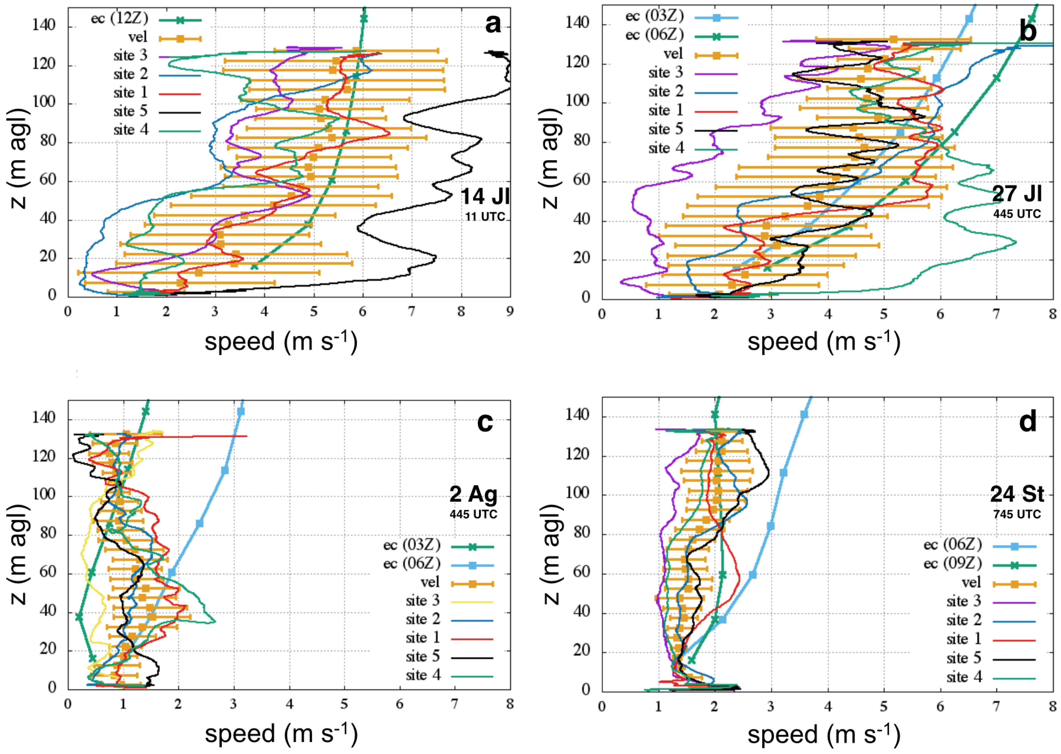
Figure 4 displays the profiles of virtual potential temperature (). For each case, the average profile of the five soundings and the corresponding spatial standard deviation bars are shown in orange. Then, each individual profile is included (the flying sequence was site 3, site 2, site 1, site 5, and site 4). Finally, the ECMWF profiles are included for the nearest grid point and the closest time intervals (extracted from the model analysis for the 12Z profiles and from the model forecasts for the other times). The same scheme is applied in Figure 5 for the wind speed. All the plots have similar ranges to facilitate comparison between the different cases.
3.1.1. A Late Morning Windy and Sunny Case (14 July 2017)
Soundings were made before solar noon, a time when the clear and windy (NW wind) convective boundary layer was evolving slowly. While profiles above agricultural and pasture surfaces are close to each other, the profile over the forest is about 1 K colder, and the one over bare agricultural soil is about 2 K warmer. The differences are sustained with height because the turbulence is able to transport heat upwards. The variability stays almost constant with height, with an approximate value for the standard deviation of close to 1 K. The ECMWF profile is close to the values over agricultural vegetated land and consequently close to the average profile, and has a small negative bulk Richardson number (Rib) indicating a weakly unstably stratified turbulent regime.
The variations of wind speed between soundings are large, due to the modification of the flow by the topography. The speed variations are sustained with height as is the standard deviation of the wind speed, close to 2 m s. The differences between soundings may be largely explained by the topographical features, which have a height similar to the vertical extent of the profiles. It is worth noting that the average profile of the wind speed observations is close to the one in the model. Furthermore, the individual profile closest to the ECMWF output is for site 1, which is the farthest from the hill, consistent with the view of the area as a gentle slope by the model.
3.1.2. A Cloudy and Windy Dawn Case (27 July 2017)
The flights were made with cloud cover and some drizzle under NW wind. Most profiles were very close in value except the one in the forest that was 2 K colder than the average inside the canopy and 1 K colder above. This profile in the forest is the one contributing to the significant dispersion in . The turbulence here is of mechanical origin in the open areas with a very weak shallow unstable layer close to the surface. Instead, in the forest canopy, the turbulence is expected to be weaker and the thermal profile to be more stable. The model profile shape compares well with the average but shows a small warm bias.
As in the 14 July case, the wind speed variability is large, related to the interaction of the flow with the topography. The average profile compares well with the ECMWF profiles. The profile in the forest (site number 3) indicates a large drag exerted by the canopy. In this case, the model’s Rib value in the first one hundred metres above the surface is close to zero but positive, indicating a turbulent regime very weakly stably stratified.
3.1.3. A Dawn Case with Clear Skies and Weak Winds (2 August 2017)
This is a weak wind case, where broken fog layers quickly dissipated followed by clear skies. The different profiles showed very slow temporal evolution, very likely because the early solar energy was evaporating liquid water from the surface. The variability of is small, showing no significant effect of the topographical variations. The weak thermal turbulence generates differences between profiles in the layers close to the surface, and the spatial variability decreases with height. The forest site is the coldest in the lower layers and has the weakest wind speed of all the profiles. Comparison with ECMWF output is good for but tends to overestimate the wind speed above the surface layer. The model has Rib values close to zero, corresponding to turbulent, weakly stable before sunset and weakly unstable afterwards.
3.1.4. A Dawn Case with Patches of Mist and Weak Winds (24 September 2017)
Dissipating mist resulted in a mixture of sunny and overcast patches, with relatively large variability of close to the surface, also influenced by weak warming as time advances. The spatial variability decreases significantly with height, especially in the stable layer above the developing but still shallow convective layer in contact with the surface. The wind is weak and shows very little variability with height, interestingly having a local maximum value near the surface, pointing to the presence of local circulations. The performance of the model is good when compared to the averaged profiles. As in the previous case, Rib is close to zero, being turbulent and weakly stable before sunrise and weakly unstable afterwards.
3.2. Quantitative Comparison of Individual Sites to Averaged and ECMWF Profiles
Figure 4 and Figure 5 indicate that there is a large variability between individual soundings and that the average of the soundings is usually centrally located and not far from the corresponding ECMWF profile. Even if each sounding is made at a different elevation, they are all averaged according to the height above ground to capture properly the surface layer and the results show that this option is meaningful. Averages using the height above sea level would have mixed surface layer profiles at high points with profiles above the surface layer in low points, providing a result with little physical sense.
The averaged profiles can be compared to the individual profiles quantitatively, as in the left part of Table 2, using the root mean-squared errors (RMSE) between pairs of profiles. Site 1 is usually the closest to the average, and we may infer that it would be the most representative of the ensemble of soundings. The forested Site 3 on the hill is the one departing the most from the average.
Determining the profile closest to the ECMWF values is relevant, especially in what concerns model initialization or validation. In the central part of Table 2, the RMSE of each profile with respect to the model values is given. The lowest error corresponds to Site 1, which is very close to the type of terrain that the model represents for the area, an open area over a gentle slope. Sites locally at more complex terrain show larger differences with the ECMWF profile, mainly in terms of the wind speed, very likely induced by the topographical perturbation on the flow by the hill.
The last column of Table 2 provides the RMSE between the model and the average of the soundings. The results are similar to those of Site 1, showing that, for this particular case study, it is almost equivalent to use the site closest to the model representation of the area or to use the average of the soundings. The generalization of such a result would need a number of experiments in varying landscapes.
3.3. A Tentative Quantification of the Surface Layer Heterogeneity
The qualitative interpretation in the previous section indicates that standard deviations may be used to estimate the heterogeneity in the surface layer. The two windy cases shown have large standard deviations for both the wind and . Instead, the less windy cases allow the thermal standard deviation to become significant while the standard deviation of the wind speed remains small, even if the value is comparable to the mean wind speed.
A heterogeneity index based on thermal and topographical variability can be constructed with the following guidelines: (i) the terrain induces variability in the flow by modifying its speed and direction, so the heterogeneity must be proportional to the terrain standard deviation ; (ii) the wind variability seems to be large if the wind speed u is significant and small for weak winds, which will be represented by ; (iii) similarly, the observed spatial variability in temperature and humidity can be summarized in terms of the standard deviation .
Combining these factors, a non-dimensional heterogeneity Thermal and Topographical index () is proposed as:
The non-dimensionality is obtained using g—the acceleration of gravity at the Earth’s surface—and , which is a reference value for the virtual potential temperature, taken here as 300 K. In this work, is computed using only surface layer values, providing a value for each of the four cases near the surface only for observational data.
The combination of factors in the non-dimensional quantity is similar but inverse to the one made to obtain the Froude number to categorize the interaction of the flow with an obstacle. is also similar to the square root of the Richardson number that represents the relative contributions of the dynamic production of turbulence and the thermal production or destruction. Therefore, can be seen as if it were the square root of a horizontal Richardson number based on horizontal thermal and dynamical variability. Furthermore, is also a measure of the ratio of the thermal response of the heterogeneity to the mechanical response to the terrain.
is a very simple parameter with room for further improvement in some aspects. For instance, as it is formulated, if the terrain vanishes (), goes to zero. The variability of the height of the surface elements could potentially be considered, using for instance the displacement height at each site, but, in our experiment, the local variability was too high to define such a quantity properly.
On the other hand, here has been computed for surface variability at the kilometre scale. However, the terrain variability happens on a variety of scales. To assess this issue, more measurements should be done at more points, but this was not possible with the available equipment. As mentioned before when discussing stationarity, the simultaneous use of several multicopter RPAS could help with inspecting this issue in future experiments. For the time being, the foreseen alternative is to compute using databases from other networks displayed at different scales.
Table 3 gives the values of for each case and the values of the standard deviations, taking for all cases = 300 K and = 40 m, a value obtained from the heights asl of the sounding locations. The value of the wind at 10 m agl is also given.
is smaller for the turbulence-dominated cases (14 and 27 July) compared to the weak-wind cases (2 August and 24 September). As expected from its definition, is small when the wind variability prevails over the thermal variability and larger when the thermal variability dominates.
The index has been developed and tested using data for a specific location. It could also be used with data from networks of surface weather stations, since the spatial variances used are computed in the surface layer.
4. Conclusions
Operating an instrumented RPAS over hilly terrain at positions with different land use and heights above sea level during four different days in quasi-stationary conditions has allowed the estimation of the spatial variability of the wind and temperature measurements at the kilometre scale. In the cases with well developed turbulence, the horizontal variability is large for wind and temperature and almost constant with height, being essentially linked to the turbulence mixing in the ABL. For the cases with weak wind and turbulence, here corresponding to early mornings, the thermal variability is largest near the surface, probably linked to the terrain height and land use variability, and decreases with height.
The variability between sites is significant, both thermally and dynamically. For sites less than 5 km apart such as the ones used in this exercise, differences can be as large as 3 m s or 3 K, depending on their position with respect to the topographical features or the land use. The site with values closest to the average of soundings was also the one closest to the ECMWF profile of the nearest grid point to the study area. In this particular case, this site was very similar in reality to the average representation of the model, a gentle slope over open terrain. The generality of these results is unknown.
This work presents the development of a methodology to inspect the variability linked to the land use and terrain heterogeneity with a RPAS. Although the sample is small, this experiment has shown that variability can be characterized and quantified, and used to understand the processes taking place in the lower ABL. The study does not intend to provide a statistical description of the variability of the area because the sample is small and not representative, but it indicates how to proceed. The simultaneous use of several RPAS could be a way to improve the methodology.
This study indicates that, when using data coming from heterogeneous terrain, only one point may be far from representativeness of the area, and create problems if used for initialization or verification of numerical models. An effort should be made to inspect the representativeness of individual model points before using them in applications.
Finally, an attempt to quantify the heterogeneity has been made combining the values of the standard deviations of wind, potential virtual temperature, and surface height in a non-dimensional parameter for the surface layer. The suggested formulation increases with the terrain and the thermal variability and decreases with the wind variability. could be computed for a network of stations to estimate the spatial variability of an area, regardless of the actual separation between measuring points.
Author Contributions
Conceptualization and methodology: J.C. and B.W.; software: B.W., B.M. and J.C.; formal analysis and validation: J.C., L.M. and B.W.; investigation: J.C., B.W. and L.M.; resources and data curation: B.W. and B.M.; writing original draft preparation: J.C.; writing—review and editing: L.M. and B.W.; project administration and funding acquisition: J.C. and B.W.
Funding
This work was funded through the projects CGL2015-65627-C3-1-R (MINECO) and RTI2018-098693-B-C31 (MICINN and AEI) of the Spanish Government, both with funding from the European Regional Development Fund (FEDER-EU). Funding from ERA-Net Plus ‘New European Wind Atlas’ project was provided by the Spanish and European Comission projects PCIN2014-016-C07-01 and PCIN-2016-091. Larry Mahrt received support from Grant AGS-1614345 from the National Science Foundation.
Acknowledgments
The authors would like to thank the municipalities of Wolfhagen und Volkmarsen for their kind support with respect to the drone operation regulations. ECMWF is thanked for providing access to data. M.A. Jiménez provided useful comments and assisted in the making of Figure 1. Reviewers are acknowledged because they have made questions and indications that have improved the quality of the manuscript substantially.
Conflicts of Interest
The authors declare no conflict of interest.
References
- Beyrich, F.; Herzog, H.J.; Neisser, J. The LITFASS project of DWD and the LITFASS-98 experiment: The project strategy and the experimental setup. Theor. Appl. Climatol. 2002, 73, 3–18. [Google Scholar] [CrossRef]
- Simó, G.; Cuxart, J.; Jiménez, M.A.; Martínez-Villagrasa, D.; Picos, R.; López-Grifol, A.; Martí, B. Observed atmospheric and surface variability on heterogeneous terrain at the hectometre scale and related advective transports. J. Geophys. Res. Atmos. 2019. [Google Scholar] [CrossRef]
- Couvreux, F.; Guichard, F.; Redelsperger, J.L.; Kiemle, C.; Masson, V.; Lafore, J.P.; Flamant, C. Water-vapour variability within a convective boundary-layer assessed by large-eddy simulations and IHOP-2002 observations. Q. J. R. Meteorol. Soc. 2005, 131, 2665–2693. [Google Scholar] [CrossRef]
- Garratt, J.R. The Atmospheric Boundary Layer; Cambridge University Press: Cambridge, UK, 1992; 334p. [Google Scholar]
- Serafin, S.; Adler, B.; Cuxart, J.; De Wekker, S.J.; Gohm, A.; Grisogono, B.; Kalthoff, N.; Kirshbaum, D.J.; Rotach, M.W.; Schmidl, J.; et al. Exchange processes in the atmospheric boundary layer over mountainous terrain. Atmosphere 2018, 9, 102. [Google Scholar] [CrossRef]
- Jackson, P.S.; Hunt, J.C.R. Turbulent wind flow over a low hill. Q. J. R. Meteorol. Soc. 1975, 101, 929–955. [Google Scholar] [CrossRef]
- Finnigan, J.J.; Belcher, S.E. Flow over a hill covered with a plant canopy. Q. J. R. Meteorol. Soc. 2004, 130, 1–29. [Google Scholar] [CrossRef]
- Brown, A.R.; Hobson, J.M.; Wood, N. Large-eddy simulation of neutral turbulent flow over rough sinusoidal ridges. Bound. Layer Meteorol. 2001, 98, 411–441. [Google Scholar] [CrossRef]
- Taylor, P.A.; Teunissen, H.W. The Askervein Hill project: Overview and background data. Bound. Layer Meteorol. 1987, 39, 15–39. [Google Scholar] [CrossRef]
- Ruck, B.; Adams, E. Fluid mechanical aspects of the pollutant transport to coniferous trees. Bound. Layer Meteorol. 1991, 56, 163–195. [Google Scholar] [CrossRef]
- Dörnbrack, A.; Schumann, U. Numerical simulation of turbulent convective flow over wavy terrain. Bound. Layer Meteorol. 1993, 65, 323–355. [Google Scholar] [CrossRef]
- Patton, E.G.; Katul, G.G. Turbulent pressure and velocity perturbations induced by gentle hills covered with sparse and dense canopies. Bound. Layer Meteorol. 2009, 133, 189–217. [Google Scholar] [CrossRef]
- Mahrt, L. Microfronts in the nocturnal boundary layer. Q. J. R. Meteorol. Soc. 2019, 145, 546–562. [Google Scholar] [CrossRef]
- Beljaars, A.C.; Brown, A.R.; Wood, N. A new parametrization of turbulent orographic form drag. Q. J. R. Meteorol. Soc. 2004, 130, 1327–1347. [Google Scholar] [CrossRef]
- Anderson, W.; Meneveau, C. Dynamic roughness model for large-eddy simulation of turbulent flow over multiscale, fractal-like rough surfaces. J. Fluid Mech. 2011, 679, 288–314. [Google Scholar] [CrossRef]
- Flack, K.A.; Schultz, M.P. Review of hydraulic roughness scales in the fully rough regime. J. Fluids Eng. 2010, 132, 041203. [Google Scholar] [CrossRef]
- Petersen, E.L.; Troen, I.; Joergensen, H.E.; Mann, J. The new European wind atlas. Energy Bull. 2014, 17, 34–39. [Google Scholar]
- Mann, J.; Angelou, N.; Arnqvist, J.; Callies, D.; Cantero, E.; Arroyo, R.C.; Courtney, M.; Cuxart, J.; Dellwik, E.; Gottschall, J.; et al. Complex terrain experiments in the new European wind atlas. Philos. Trans. R. Soc. A 2017, 375, 20160101. [Google Scholar] [CrossRef] [PubMed]
- Künt, P.; Basse, A.; Callies, D.; Chen, Y.; Döpfer, R.; Freier, J.; Griesbach, T.; Klaas, T.; Pauscher, L. NEWA Forested Hill Experiment: Experiment Documentation; Technical Report IEE-2018-214-V2; Fraunhofer-Gesellschaft: München, Germany, 2018; 72p. [Google Scholar]
- Pauscher, L.; Callies, D.; Klaas, T.; Foken, T. Wind observations from a forested hill: Relating turbulence statistics to surface characteristics in hilly and patchy terrain. Meteorol. Z. 2018, 27, 43–57. [Google Scholar] [CrossRef]
- Debor, S. Multiplying mighty Davids. In The Influence of Energy Cooperatives on Germany’s Energy Transition; Springer: Berlin/Heidelberg, Germany, 2018. [Google Scholar]
- Wrenger, B.; Cuxart, J. Evening transition by a river sampled using a remotely-piloted multicopter. Bound. Layer Meteorol. 2017, 165, 535–543. [Google Scholar] [CrossRef]
- Prohasky, D.; Watkins, S. Low Cost Hot-element Anemometry Verses the TFI Cobra. In Proceedings of the 19th Australasian Fluid Mechanics Conference, Melbourne, Australia, 8–11 December 2014. [Google Scholar]
- Neumann, P.P.; Bartholomai, M. Real-time wind estimation on a micro unmanned aerial vehicle using its inertial measurement unit. Sens. Actuator A Phys. 2015, 235, 300–310. [Google Scholar] [CrossRef]
Figure 1.
(Top left): topography of the area surrounding Rödeser Berg at a resolution of 90 m (approx. 35 km E–W × 25 km N–S); (top right): detailed topography and terrain uses at Rödeser Berg (6 km × 6 km), green represents woods; (bottom left): topography at a resolution of 90 m in a larger area (approx. 60 km E–W × 80 km N–S); (bottom right): the same but at a resolution of 9 km as seen by the European Centre for Medium-Range Weather Forecasts (ECMWF) model.

Figure 2.
(Above): horizontal topographical profile across Rödeser Berg between Site 1 and Site 4, crossing Site 2. (Below): topographical profile along the ridge of Rödeser Berg, between Site 3 and Site 5.
Figure 2.
(Above): horizontal topographical profile across Rödeser Berg between Site 1 and Site 4, crossing Site 2. (Below): topographical profile along the ridge of Rödeser Berg, between Site 3 and Site 5.

Figure 3.
Q13 Remotely Piloted Aircraft System (RPAS) with a sensor mast horizontally attached. The length of the mast is suitable to prevent a significant impact by the multicopter’s downwash.
Figure 3.
Q13 Remotely Piloted Aircraft System (RPAS) with a sensor mast horizontally attached. The length of the mast is suitable to prevent a significant impact by the multicopter’s downwash.

Figure 4.
Virtual potential temperature profiles for each experimental case. The thin lines represent individual soundings. Orange profiles correspond to the average profiles and the standard deviation. The thicker blue and green lines with points are the ECMWF outputs for the nearest model grid point and time. (a) soundings on 14 July 2017 between 10:17 and 11:51 UTC; (b) 27 July between 3:44 and 5:31 UTC; (c) 2 August between 4:02 and 5:25 UTC; (d) 24 September between 7:10 and 8:15 UTC. In the figure, the central times for each case are approximately given.

Figure 5.
As in Figure 4 for the wind speed.
Figure 5.
As in Figure 4 for the wind speed.


Table 1.
Physical characteristics of the sounding locations.
| Site (lat/lon) | Elevation (m) | Use of Terrain | Vegetation Height (m) | Dist to 1, 2, 3, 4, 5 (km) |
|---|---|---|---|---|
| 1 (51.337 N/9.168 E) | 263 | agr bare/veg | 0–1 | x, 1, 5, 5, 3 |
| 2 (51.344 N/9.178 E) | 231 | agr vegetated | 0.5 | 1, x, 4, 4, 2 |
| 3 (51.377 N/9.169 E) | 218 | forest | 15–20 | 5, 4, x, 2, 5 |
| 4 (51.373 N/9.202 E) | 268 | agr bare | 0 | 5, 4, 2, x, 3 |
| 5 (51.348 N/9.213 E) | 321 | pasture | 0.1 | 3, 2, 5, 3, x |
Table 2.
Root mean squared error (RMSE) of each site in respect to the average of sites (five left columns), RMSE of each site and of the average in respect the European Centre for Medium-Range Weather Forecasts (ECMWF) model profile (next five columns). The RMSE value of the virtual potential temperature is the upper value of each cell (in K), and the lower one is the wind speed (in m s. The last numerical column displays the RMSE between the average of sites and the ECMWF profile.
| Case | s1-av | s2-av | s3-av | s4-av | s5-av | s1-ec | s2-ec | s3-ec | s4-ec | s5-ec | av-ec | |
|---|---|---|---|---|---|---|---|---|---|---|---|---|
| 14 July | 0.49 | 0.66 | 1.04 | 0.37 | 1.99 | 0.89 | 0.78 | 1.36 | 0.46 | 1.80 | 0.42 | K |
| 0.66 | 2.18 | 1.51 | 1.32 | 3.02 | 0.84 | 2.85 | 1.94 | 1.88 | 2.60 | 0.79 | m s | |
| 27 July | 0.36 | 0.17 | 1.59 | 0.63 | 1.03 | 1.10 | 1.37 | 3.00 | 0.79 | 0.42 | 1.42 | K |
| 1.01 | 1.20 | 2.15 | 2.39 | 0.94 | 0.96 | 0.88 | 3.18 | 1.93 | 1.69 | 1.19 | m s | |
| 2 August | 0.50 | 0.96 | 0.76 | 0.21 | 0.23 | 0.75 | 1.07 | 0.95 | 0.42 | 0.43 | 0.37 | K |
| 0.22 | 0.60 | 1.06 | 0.24 | 0.72 | 0.74 | 0.56 | 0.72 | 0.96 | 0.88 | 0.79 | m s | |
| 24 September | 0.69 | 1.53 | 1.62 | 0.43 | 0.08 | 1.20 | 1.32 | 1.36 | 1.77 | 1.50 | 1.46 | K |
| 0.40 | 0.28 | 0.92 | 0.65 | 0.19 | 0.42 | 0.58 | 1.17 | 0.94 | 0.45 | 0.32 | m s | |
| Average | 0.51 | 0.83 | 1.25 | 0.41 | 0.83 | 0.99 | 1.13 | 1.67 | 0.86 | 1.04 | 0.92 | K |
| 0.57 | 1.06 | 1.41 | 1.15 | 1.22 | 0.74 | 1.22 | 1.75 | 1.43 | 1.40 | 0.78 | m s |
Table 3.
Selected characteristics of the experimental cases. u10 is the wind speed at a height of 10 m above the surface, the standard deviations are computed with values of the 5 sites at 2 m above the surface, and stands for ’Heterogeneity Thermal and Topographical index’.
Table 3.
Selected characteristics of the experimental cases. u10 is the wind speed at a height of 10 m above the surface, the standard deviations are computed with values of the 5 sites at 2 m above the surface, and stands for ’Heterogeneity Thermal and Topographical index’.
| Date and Time (UTC) | Weather | u10 (m/s) | (m/s) | (K) | |
|---|---|---|---|---|---|
| 14 July, 10:17–11:51 | clear CBL | 3 | 2 | 1.5 | 0.70 |
| 27 July, 3:44–5:31 | drizzle | 3 | 2 | 1.2 | 0.62 |
| 2 August, 4:04–5:25 | broken, dew | 1 | 0.2 | 0.5 | 4.03 |
| 24 September, 7:10–8:15 | fading mist | 1.2 | 0.2 | 1.5 | 7.06 |
© 2019 by the authors. Licensee MDPI, Basel, Switzerland. This article is an open access article distributed under the terms and conditions of the Creative Commons Attribution (CC BY) license (http://creativecommons.org/licenses/by/4.0/).
Share and Cite
MDPI and ACS Style
Cuxart, J.; Wrenger, B.; Matjacic, B.; Mahrt, L. Spatial Variability of the Lower Atmospheric Boundary Layer over Hilly Terrain as Observed with an RPAS. Atmosphere 2019, 10, 715. https://0-doi-org.brum.beds.ac.uk/10.3390/atmos10110715
AMA Style
Cuxart J, Wrenger B, Matjacic B, Mahrt L. Spatial Variability of the Lower Atmospheric Boundary Layer over Hilly Terrain as Observed with an RPAS. Atmosphere. 2019; 10(11):715. https://0-doi-org.brum.beds.ac.uk/10.3390/atmos10110715
Chicago/Turabian StyleCuxart, Joan, Burkhard Wrenger, Blazenka Matjacic, and Larry Mahrt. 2019. "Spatial Variability of the Lower Atmospheric Boundary Layer over Hilly Terrain as Observed with an RPAS" Atmosphere 10, no. 11: 715. https://0-doi-org.brum.beds.ac.uk/10.3390/atmos10110715
Note that from the first issue of 2016, this journal uses article numbers instead of page numbers. See further details here.