Measuring Regional Atmospheric CO2 Concentrations in the Lower Troposphere with a Non-Dispersive Infrared Analyzer Mounted on a UAV, Ogata Village, Akita, Japan

Chiba, Takashi; Haga, Yumi; Inoue, Makoto; Kiguchi, Osamu; Nagayoshi, Takeshi; Madokoro, Hirokazu; Morino, Isamu

doi:10.3390/atmos10090487

Open AccessArticle

Measuring Regional Atmospheric CO₂ Concentrations in the Lower Troposphere with a Non-Dispersive Infrared Analyzer Mounted on a UAV, Ogata Village, Akita, Japan

¹

Faculty of Bioresource Sciences, Akita Prefectural University, Akita 010-0195, Japan

²

Graduate School of Bioresource Sciences, Akita Prefectural University, Akita 010-0195, Japan

³

Faculty of Systems Sciences and Technology, Akita Prefectural University, Yurihonjo 015-0055, Japan

⁴

National Institute for Environmental Studies, Tsukuba 305-8506, Japan

^*

Author to whom correspondence should be addressed.

Atmosphere 2019, 10(9), 487; https://0-doi-org.brum.beds.ac.uk/10.3390/atmos10090487

Submission received: 2 July 2019 / Revised: 17 August 2019 / Accepted: 20 August 2019 / Published: 23 August 2019

(This article belongs to the Special Issue Applications of Small Unmanned Aerial Systems (sUAS) in Atmospheric Chemistry and Physics)

Download

Browse Figures

Versions Notes

Abstract

:

We have developed a simple measuring system prototype that uses an unmanned aerial vehicle (UAV) and a non-dispersive infrared (NDIR) analyzer to detect regional carbon dioxide (CO₂) concentrations and obtain vertical CO₂ distributions. Here, we report CO₂ measurement results for the lower troposphere above Ogata Village, Akita Prefecture, Japan (about 40° N, 140° E, approximately −1 m amsl), obtained with this UAV system. The actual flight observations were conducted at 500, 400, 300, 200, 100, and 10 m above the ground, at least once a month during the daytime from February 2018 to February 2019. The raw CO₂ values from the NDIR were calibrated by two different CO₂ standard gases and high-purity nitrogen (N₂) gas (as a CO₂ zero gas; 0 ppm). During the observation period, the maximum CO₂ concentration was measured in February 2019 and the minimum in August 2018. In all seasons, CO₂ concentrations became higher as the flight altitude was increased. The monthly pattern of observed CO₂ changes is similar to that generally observed in the Northern Hemisphere as well as to surface CO₂ changes simulated by an atmospheric transport model of the Japan Meteorological Agency. It is highly probable that these changes reflect the vegetation distribution around the study area.

Keywords:

carbon dioxide (CO₂); non-dispersive infrared (NDIR) analyzer; unmanned aerial vehicle (UAV); observation method; Akita; Japan

1. Introduction

Increases in greenhouse gases such as carbon dioxide (CO₂) in the atmosphere have contributed to rising global air temperatures in recent years. Before the Industrial Revolution, the CO₂ concentration in Earth’s atmosphere was approximately 280 ppm, and it has been gradually but steadily increasing since then [1,2]. The CO₂ concentration has increased by about 1–2 ppm per year since the 1950s; consequently, the global annual mean CO₂ concentration exceeded 400 ppm in 2015 [3]. However, accurate estimation of the carbon balance between ecosystem absorption and emission from ground surfaces (e.g., green carbon) and clarification of the relationship between atmospheric concentrations and topographic features and land use are necessary [4,5]. To clarify the detailed distribution of CO₂ sources and sinks, however, accurate vertical CO₂ profile measurements, including the lower troposphere over various locations, are needed. Global CO₂ observations using satellite remote sensing have been conducted with the Infrared Atmospheric Sounding Interferometer (IASI) [6], the Atmospheric Infrared Sounder (AIRS) [7], the Greenhouse gases Observing SATellite (GOSAT) [8], and the Orbiting Carbon Observaroy-2 (OCO-2) [9]. However, satellite measurements make it difficult to obtain accurate CO₂ concentrations in the lower troposphere below 500 m. Vertical CO₂ concentration profiles have been measured from several in situ platforms, including tall towers e.g., [10,11], aircraft e.g., [12,13,14], and balloons e.g., [15,16]. Measurements of the CO₂ concentration in the stratosphere using balloon-borne cryogenic samplers have been conducted over Japan since 1985 for understanding the global carbon cycle [15]. Although these measurements provide comprehensive information on CO₂ concentrations in the atmosphere, regional distributions of CO₂ sources and sinks are still uncertain in many areas because of the sparseness of available vertical profile observations. Moreover, these measurement methods are usually expensive, and mostly they can be used only at a limited number of observation sites. Although advanced space/time geostatistical modeling, used in many water and air quality studies, can be a helpful for CO₂ 3-D space/time interpolation, it may not be the most suitable framework for accurate CO₂ estimation e.g., [17,18]. To investigate local CO₂ distributions, measurements must be made frequently and simultaneously in multiple locations. In addition, because aircraft measurements can be employed over only a limited altitudinal range (about 0.5–12 km above the surface), alternative methods for measuring CO₂ concentrations in the lower troposphere below 500 m are needed.

Recently, unmanned aerial vehicles (UAVs) have started to be used as a tool for routine meteorological and atmospheric observations e.g., [19,20,21,22,23,24,25,26,27]. We have developed a prototype of a simple measurement system that uses a UAV and a non-dispersive infrared (NDIR) analyzer to measure atmospheric CO₂ concentrations [28,29,30]. Although UAVs have altitude limits, our prototype system can be used to easily and inexpensively obtain vertical CO₂ profiles in the lower troposphere below 500 m. To acquire such a profile by balloon observations takes 1–2 h, depending on weather conditions [31], whereas our UAV system can do so in about 20 min. Therefore, the use of a UAV for measurements makes it possible to investigate vertical CO₂ concentrations in the atmospheric boundary layer at a fine temporal resolution (e.g., hourly) and to detect diurnal CO₂ variations. Additionally, CO₂ data can be obtained over various sites through optimal adjustment of the location and altitude of the UAV. In this paper, we present the results of vertical CO₂ concentration measurements obtained with this system in Ogata Village Akita, Japan, from February 2018 to February 2019.

2. Materials and Methods

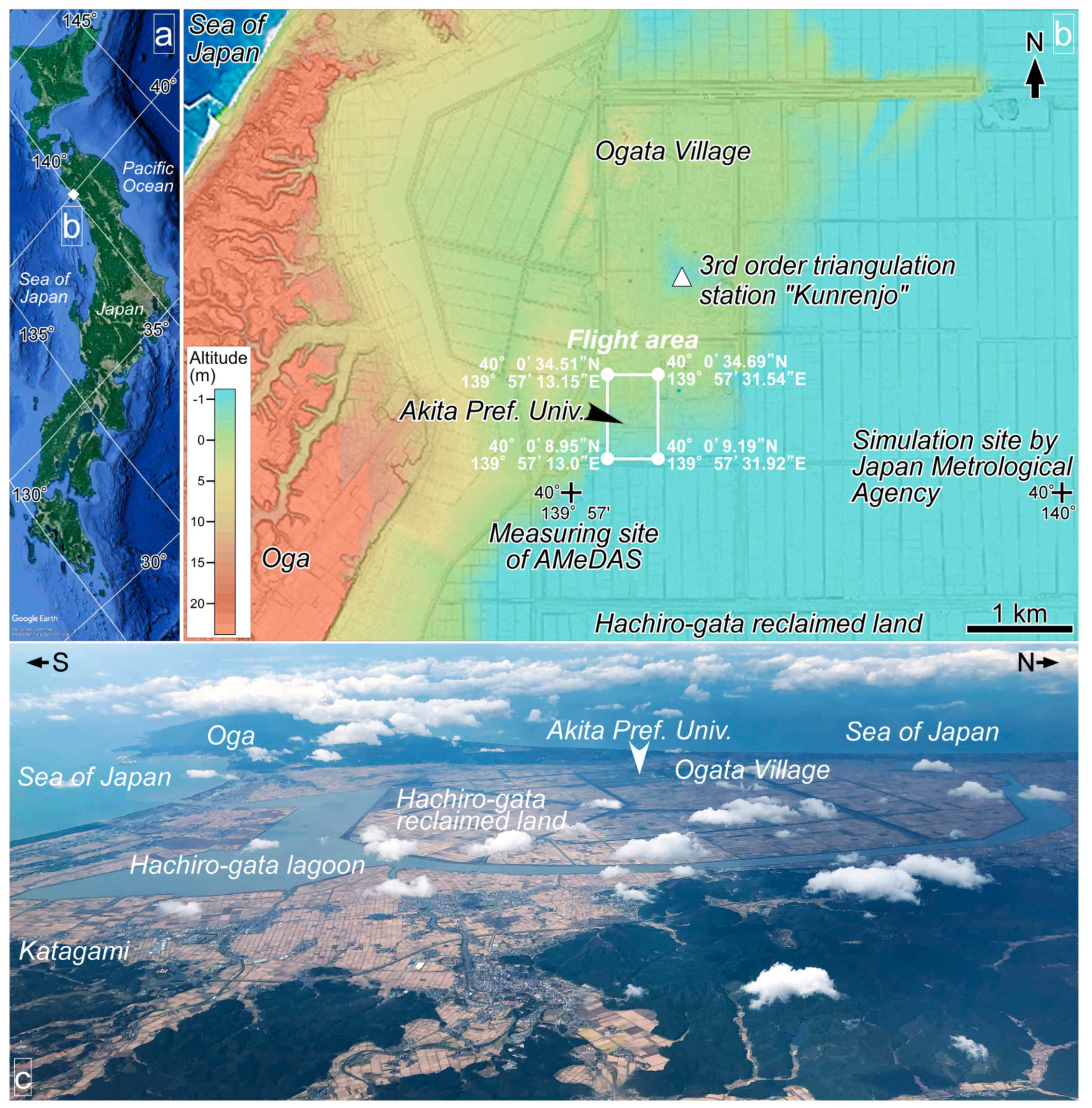
2.1. CO₂ Measurement Site

The selected flight area is 5 km inland from the Japan Sea coast in a vast farmland area consisting of flat reclaimed land (Figure 1). Ogata Village consists mostly of agricultural lands, and no large sources of greenhouse gas emissions, such as powerplants and factories, are nearby. Prevailing wind directions are typically south and west, according to records collected by the Automated Meteorological Data Acquisition System (AMeDAS) station at Ogata [32]. Secular changes in CO₂ concentrations near the flight area, in Ogata Village (about 40° N, 140° E) (Figure 1), have been calculated and simulated by the Global Spectral Atmosphere Model-Transport Model (GSAM-TM) of the Japan Meteorological Agency (JMA) [33,34] (Figure 2). In this study, we compared the CO₂ data obtained by the UAV with these monthly simulated CO₂ data (see Section 2.4).

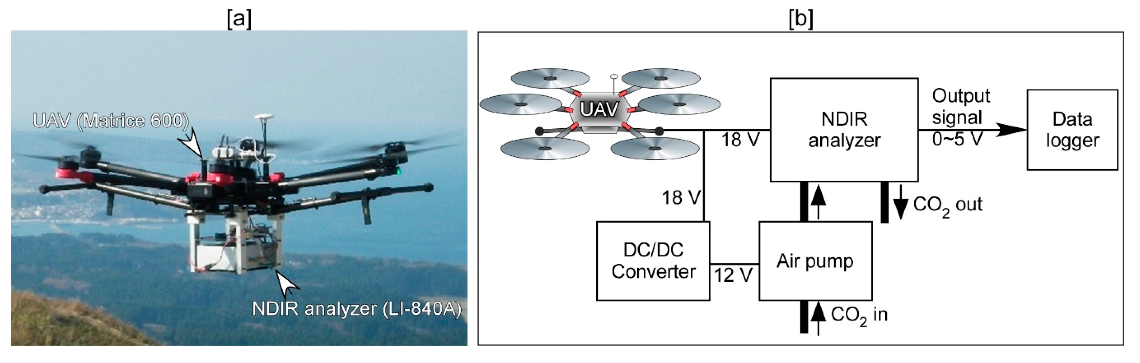
2.2. CO₂ Measurements Using UAV System

We measured CO₂ concentrations with a UAV system developed by Madokoro et al. [28], Inoue et al. [29], and Nomura et al. [30] (Figure 3). The Matrice 600 UAV (DJI) and LI-840A NDIR analyzer (LI-COR) used in this study cost about 0.5 million yen and 1.6 million yen, respectively, and their specifications are given in Table 1 and Table 2, respectively. The Matrice 600 is a relatively large UAV without stringent payload limitations (6.0 kg). It therefore can accommodate the NDIR analyzer and the other accessories. The maximum ascent speed is 5.0 m/s, and the maximum descent speed is 3.0 m/s. The flight control system is built with the Matrice 600 for accurate and stable flight performance. The LI-840A NDIR analyzer is reliable under the cold temperatures at 500 m altitude in the lower troposphere (approximately 3 °C colder than at ground level). It is not equipped, however, with either an air pump to take in the outside air or a data recording device. For this reason, a diaphragm-type pump driven by a 12-V DC motor was attached to the system, and a voltage logger (LR 5062; HIOKI Corporation, Table A1) was used to record the data. The NDIR, pump, and data logger were attached to the drone using a dedicated mount (Figure 3). A dedicated harness for power distribution was constructed, and the 18-V output from the drone was stepped down to 12 V via a DC/DC converter to supply power to the pump.

The total loaded weight was 2.7 kg. To minimize the total weight of the UAV system, the NDIR was directly wired to the power source in the main body of the UAV; that is, an alternative power source for the NDIR was not provided.

The observation site elevation (i.e., ground level), measured by a total station (GPT-9005A, TOPCON) using the third order triangulation station (Table A2), was approximately 1 m below Tokyo Peil (T.P., the standard datum for Japan, +0.9 m relative to mean sea level in Tokyo Bay; Geospatial Information Authority of Japan). Flight observations were conducted at 500, 400, 300, 200, 100, and 10 m above the ground for 30 s at each altitude; at least one observation was conducted during the daytime each month from February 2018 to February 2019. The meteorological information for the UAV flight time on each survey date, given in Table 3, is based on hourly station data at Ogata provided by the JMA. The surface sunshine duration data are expressed in hours per hour. For example, if there were 12 min of sunshine between 10:00 a.m. and 11:00 a.m., then the sunshine duration at 11:00 a.m. would be 0.2. Observations were not made while precipitation was occurring, but otherwise they were made over a wide range of weather conditions (Table 3).

In general, the air density of the atmosphere thins with increasing altitude. As a result, the quantity of air entrained into the NDIR as the UAV moves through the air is smaller during the UAV’s descent than during its ascent. Hence, contamination of measured CO₂ concentrations by CO₂ from higher altitudes is considered to be less during the UAV’s descent than during its ascent. To clarify this point, we compared the standard deviations of CO₂ concentrations measured during 3 min at the respective altitudes between the UAV’s ascent and descent. This comparison showed that on 10 and 29 August 2018, for example, the standard deviations of concentrations measured near the ground and at 500 m altitude were larger during the ascent (see Table A3 and Table A4 for details). In fact, the standard deviation was generally smaller during the descent than during the ascent (Figure A1). Therefore, we adopted the CO₂ values observed as the UAV descended in this study. The forests and farmlands around the observation site can act as CO₂ sources or sinks and therefore can cause CO₂ concentrations to fluctuate. However, from nighttime to early morning, a temperature inversion, when cool air near the ground is overlain by a layer of warmer air in surfaces [36], is occasionally observed around Ogata Village. For example, according to temperature profile data at Akita city provided by the JMA, on 20 September 2018, at 9:00 a.m. Japan Standard time (JST; JST = UTC + 9 h), air temperatures at altitudes of 7 and 137 m were 18.3 and 16.5 °C, respectively, whereas at 9:00 p.m. JST, air temperatures at altitudes of 7 and 133 m were 18.7 and 18.9 °C, respectively. An inversion limits the diffusion of gases and leads to the accumulation of CO₂ near the surface. Therefore, to avoid any influence from a temperature inversion on the measurement results, observations were conducted between 11:00 a.m. and 4:00 p.m. JST during spring and autumn and between 11:00 a.m. and 3:00 p.m. JST in winter.

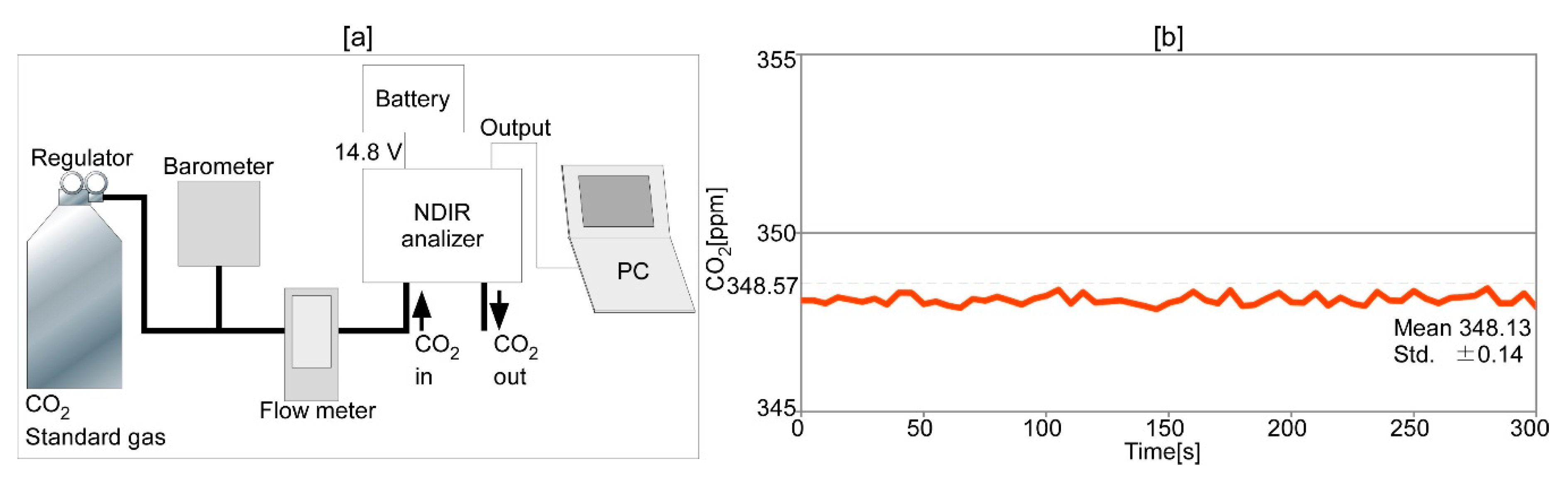
2.3. CO₂ Calibration and Measurement Uncertainty

Our UAV system continuously detects CO₂ concentrations with an NDIR gas analyzer. Measurements by NDIR require the use of standard gases defined against an absolute calibration system [37]. We therefore prepared three standard gases (Japan Fine Products), a high-purity nitrogen (N₂) gas (as a CO₂ zero gas; 0 ppm), and two CO₂ standard gases, one with high CO₂ (>390 ppm) and the other with low CO₂ (<390 ppm), which we used to relate the responses of the analyzer to absolute CO₂ concentrations. Before the flight, these standard gases were injected into the NDIR on the ground for calibration of the CO₂ concentrations measured during the flight, as described previously [38]. Figure 4 shows an example of measured concentrations of a CO₂ standard gas after calibration of the NDIR.

The LI-840A NDIR has an internal pressure transducer for pressure compensation (pressure compensation range: 150–1150 hPa). The average air pressure at sea level is 1013 hPa, and air pressure at 500 m above sea level (i.e., the maximum altitude of our UAV flights) is approximately 955 hPa. We estimated the effects of atmospheric pressure on the CO₂ measurements under a constant air flow rate (2.2 L/min) in the laboratory. We evaluated the CO₂ concentrations obtained by the LI-840A NDIR under pressures of 690–796 Torr (approximately 920–1061 hPa, measured by a 375 Convectron Vacuum Gauge Controller; Helix Technology Corporation) using a CO₂ standard gas with a concentration of 348.57 ppm and found that the measured CO₂ concentrations were almost constant. We also used a mass flow meter (MODEL RK1600R; COFLOC) to evaluate the influence of the air flow rate on CO₂ measurements by the LI-840A NDIR. Specifically, we compared CO₂ concentrations obtained by the NDIR under a flow rate 2.8 L/min with those obtained under a flow rate 1.0 L/min. The results showed a difference of approximately 1.0 ppm between concentrations measured at the two flow rates. The sensitivity of the CO₂ concentration to the atmospheric water vapor content is less than 0.1 ppm [39].

To estimate the effects of the rotation of the UAV’s propellers on CO₂ detection, we also measured the CO₂ concentrations for 30 s twice while the propellers were rotating and two more times while they were stopped. The mean CO₂ concentrations and standard deviations measured while the propellers were rotating were 384.54 ± 0.36 and 387.03 ± 0.87 ppm, and those measured while they were stopped were 385.58 ± 0.31 and 388.16 ± 0.87 ppm. Therefore, the measured CO₂ concentration was approximately 1 ppm lower when the propellers were rotating than when they were stopped (Table A6).

2.4. CO₂ Simulation

We used monthly mean global CO₂ concentration data simulated by JMA [33] to calculate the mean annual trend of CO₂ around the observation site. The JMA has operationally conducted atmospheric inversion analysis using the Carbon Dioxide Transport Model (CDTM) since 2009 [40,41], and the JMA recently updated its operational inversion analysis system to the newly developed Global Spectral Atmosphere Model-Transport Model (GSAM-TM) [33,34]. The transport process of GSAM-TM is directly coupled with a low-resolution version of JMA’s operational global numerical weather prediction (NWP) model, which has a horizontal resolution of TL95 (approximately 1.875°) with 60 vertical layers up to 3 hPa. Comparison with observation data has shown that the newly developed GSAM-TM is better able to reproduce temporal fluctuations in the boundary layer than the CDTM, though surface CO₂ simulation data seem to be slightly higher than observations [34].

We calculated the mean annual trend to be approximately 1.9 ppm/yr during 1985–2017 (Figure 2) and used this annual trend to estimate monthly CO₂ concentrations near the observation site during the observation months in 2018–2019 for comparison with the UAV data.

3. Results

From February 2018 to February 2019, a total of 19 vertical profiles were obtained (Table A3 and Table A4). For every observation, the standard deviation was within 1.75 ppm (Figure 5). The meteorological conditions on each observation date recorded by the AMeDAS station at Ogata [32] are listed in Table 3.

Vertical CO₂ concentration gradients during the cold season (February–March 2018, December 2018, and January–February 2019) around Ogata Village tend to be small from the ground surface to an altitude of 500 m, and the differences in the CO₂ concentration at a given altitude were within 1.0 ppm. The CO₂ concentration gradients from the ground surface to 500 m above the ground surface were less noticeable during April and May 2018, although slightly higher concentrations were observed at higher altitudes than during the summer periods. However, on 28 May 2018, the vertical CO₂ gradient was large at altitudes of 300–500 m. From June to August 2018, noticeable vertical gradients, namely, low concentrations near the ground surface and high concentrations at higher altitudes, were observed. In July and August 2018, CO₂ concentrations at 10 m altitude were about 4–6 ppm smaller than those at 100 m altitude. From September to November 2018, the CO₂ concentration gradients up to 500 m were less noticeable, although slightly higher concentrations were observed with increases in altitude. The vertical profiles and the concentration gradients observed from April to May 2018 were similar to those observed from September to November 2018.

Focusing on the seasonal behavior of CO₂ in the lower troposphere, we found that the CO₂ concentrations over Ogata became lower from June to midsummer (Figure 5c). This result may primarily reflect increased photosynthesis due to the longer duration of sunshine. The rapid increase of CO₂ concentrations from September to October and from December to January might also be explained by changes in the vegetation distribution with the seasonal evolution (Figure 5a,d).

Figure 6 shows the seasonal variations of CO₂ concentrations at each measurement altitude. At all altitudes, CO₂ concentrations decreased from spring to summer and rose from autumn to winter. A local CO₂ concentration maximum was observed in February 2019, and minimum concentrations were observed in August 2018. The seasonal fluctuations were the largest near the ground surface (i.e., at 10 m) and tended to be smaller at higher altitudes. Furthermore, the CO₂ concentration increased rapidly from October to November 2018. After that, it temporarily decreased in January 2019, but it then increased again to a maximum in February 2019. On the other hand, when comparing the surface simulation results for 40° N, 140° E in the GSAM-TM results (dashed line in Figure 6) and the corrected values, the rough trends of the changes coincided, but many observed values were below the simulation values. The difference in CO₂ concentrations between the GSAM-TM results and the measured results was greater in the summer period. For example, the simulation results and their correction values were 415.8, 400.6, and 410.7 ppm in February, August, and October 2018, respectively (Figure 2 and Figure 6), while the observation results were 414.94 ± 0.15, 377.25 ± 0.34, and 406.94 ± 0.37 ppm on 26 February, 29 August, and 12 October 2018, respectively (Table A3 and Figure 6).

4. Advantages and Disadvantages of UAV/NDIR System and the Other Platforms

As noted in Section 1, several in situ platforms, such as meteorological towers, aircraft, and balloons, have been used to obtain the vertical CO₂ concentration data. Here we discuss the advantages and the disadvantages of measurement methods by the UAV system and other platforms.

Owing to the limitation of available flight time (about 20 min with payload), it is difficult to measure CO₂ concentrations above the middle troposphere (e.g., 3 km) by our UAV system. The tower measurements by the JMA were conducted until 200 m altitude [10]. On the other hand, the aircraft and balloon observations can be performed over at least 12 and 30 km, respectively. The UAV is not suitable for the CO₂ measurements at higher altitudes.

We next focus on the validity of local CO₂ observations. To obtain the vertical CO₂ data at a certain location by aircraft, it is necessary to conduct a horizontal flight at a broad area over several kilometers. To avoid the accidents associated with falling into the urban area, the balloon system is thrown away in the ocean after the flight owing to long-distance transportation (e.g., 100 km) by strong westerly winds [42]. Thus, it is difficult to obtain the CO₂ profile data almost vertically at a site using aircraft and balloons. The meteorological tower is more suitable for the vertical CO₂ measurements, despite the number of available measurement locations being limited. For the UAV measurements, optimal adjustment of the location and altitude enables us to obtain the vertical CO₂ data over a confined area. We therefore consider that the UAV is useful for observing the local CO₂ concentrations.

The suitability of routine and continuous observations has also been discussed. The balloon observations rely on gases such as hydrogen and helium to elevate weather balloons. Helium gases, in particular, are often used owing to the growth concerns on hydrogen safety. However, it is difficult to employ frequent balloon measurements when there is a shortage of helium. In an example of aircraft measurements, the cost of charter aircraft was extremely high (e.g., about several million yen per flight day) [29,38]. It is difficult to conduct CO₂ observation using aircraft frequently and continuously. Basically, the frequent CO₂ measurements by the UAV can be performed only by preparing a full set of UAV and NDIR analyzers. The continuous UAV measurements can lead to the detection of the features of long-term variabilities, including seasonal and annual behaviors.

5. Features of Monthly CO₂ Concentrations Measured by the UAV System

The highest CO₂ concentration during the observation period was observed on 25 February 2019 (422.37 ppm at 500 m), and the lowest was observed on 29 August 2018 (377.25 ppm at 10 m) (Figure 5). During 2018, the monthly changes showed a decreasing trend from winter to summer and an increasing trend from summer to winter. In addition, during most seasons, the CO₂ concentrations measured by the NDIR increased with altitude. Although changes in the flow rate of the air pump and in barometric pressure must be considered, the influence of land use, namely, agricultural crops and natural vegetation growing on Ogata Village farmlands, may be strong, as discussed below. These observed monthly CO₂ variations in Ogata Village are similar to those reported by previous studies [43,44] conducted in the Northern Hemisphere as well as to surface simulation results for 40° N, 140° E in the GSAM-TM results (dashed line in Figure 6).

The results show that regional atmospheric CO₂ concentration changes are variable: seasonal fluctuations in the vicinity of the ground (10 m above the ground) were the most prominent, and the maximum fluctuation range from summer 2018 to winter 2019 was greater than 40 ppm. These results probably reflect the effects of vegetation in the area surrounding the flight observation site. From February to March and in December 2018, and in January and February 2019, CO₂ concentration gradients from near the ground surface up to 500 m were small. Therefore, in winter, Ogata Village may not be a site of notable CO₂ emission or absorption compared with the surrounding area. However, the CO₂ concentration from April to October 2018 tended to be lower near the ground surface and higher at higher altitudes. From June to August in particular, a large concentration decrease was observed from 10 to 100 m. This result suggests that during the summer, CO₂ near the ground surface was being absorbed. At Ogata [32], the temperature increases with the seasonal progression from spring to summer, and the hours of sunshine also increase (Table 3 and Figure 6). The lowest CO₂ concentration was observed at the end of August, when air temperature was higher, and the daylight hours were longer than in other months (Figure 6). This result may be related to increased CO₂ absorption due to enhanced photosynthetic activity. Sasakawa et al. [11] investigated vertical CO₂ concentration distributions acquired by tower and aircraft observations in the vast forested area (taiga) of Siberia and found that, because of photosynthetic activity, vertical CO₂ concentration profiles during the daytime in summer showed markedly lower values near the ground surface. The characteristics of the vertical CO₂ concentration profiles during summer around Ogata Village are consistent with their results [11].

Moreover, it is possible to distinguish short-term fluctuations (of less than 1 month duration) from long-term (seasonal) fluctuations. For example, the vertical gradient from 300 to 500 m was particularly large on 28 May 2018. In general, CO₂ is a chemically stable gas that is not formed or degraded in the atmosphere [36]. Moreover, in midlatitude synoptic systems, the vertical scale of wind speed changes is small, differing from changes on the horizontal scale by two orders of magnitude [45]. Thus, it may be that the steep vertical CO₂ gradient observed on 28 May reflects horizontal advection of an air mass enriched in CO₂ from another area, such as an urban area or Eurasia.

To clarify the formation process of the vertical CO₂ profiles, it is important to evaluate the effect of the turbulence in the lower atmosphere on the local CO₂ distribution. However, the UAV did not have observation devices for measuring vertical profiles of meteorological variables such as wind, air temperature, and humidity. It would be desirable to use the UAV system to measure turbulent 3D wind vectors and other meteorological data [46,47]. In addition, the observed CO₂ concentrations were generally lower than the simulated surface values [33] (Figure 6). This result is similar to the previous study on the GSAM-TM [34]. Moreover, the seasonal change in CO₂ concentrations was not symmetrical about the summertime minimum (Figure 6): the CO₂ concentration increase in autumn occurred more rapidly than the decrease during the previous summer. The period from September to November is the rice harvest period [48,49] (Table A7), and open burning is used to clear some rice paddy fields in Ogata Village. These results show that regional atmospheric CO₂ concentration fluctuations are variable and complicated. Therefore, accurate estimates of the amounts of CO₂ absorbed and released at the ground surface are needed [50]. The reasons for some CO₂ fluctuations will be made clear by conducting simultaneous atmospheric observations and comparative verifications at multiple sites. Although both seasonal and regional-scale fluctuations occur, they are not necessarily representative of CO₂ concentration increases due to topography and land use, so it is likely that regional-scale observations such as UAV observations will become more important in the future.

6. Conclusions

To easily and efficiently measure the regional CO₂ concentrations in the atmosphere, we developed a simple measuring system prototype that uses a UAV and an NDIR, and we applied this system to obtain the CO₂ concentrations at 500, 400, 300, 200, 100, and 10 m above the ground in Ogata Village, Akita Prefecture, Japan, from February 2018 to February 2019. Comparison with CO₂ simulation results by the JMA showed that the system made it possible to conveniently determine vertical CO₂ concentration profiles and seasonal changes in CO₂ concentrations. In a surface environment that is also susceptible to local influences such as distribution of vegetation, and therefore, subject to change in varying CO₂ concentrations (Figure 5), the accuracy of the simulation model is likely to improve by performing atmospheric observations using UAVs at more points and more frequently. To validate the vertical CO₂ data obtained by the UAV system, further studies are required that compare UAV observations with simultaneous observations made from other platforms, such as balloons, towers, and aircraft, in the designated region. At present, the maximum flight ceiling set by the application software provided by DJI restricts UAV flights to altitudes below 500 m. In the future, the use of third-party-provided software will allow observations above 500 m altitude to be performed by the UAV system. Moreover, it may be possible in the future to estimate differences in carbon absorption/fixation related to land use by combining data on vegetated areas determined by GIS, CO₂ absorption/fixation values obtained by the chamber method, and high-resolution drone observations, although atmospheric drone observations are not strictly comparable to chamber observations or simulated results.

Author Contributions

M.I. proposed the concept and took on the project administration. T.C. performed investigations and analysis, and wrote the original draft. Y.H. performed formal analysis and investigations. T.N. performed investigations and participated in discussions. O.K., H.M. and I.M. contributed to the writing—review, and participated in discussions.

Funding

This work was supported in part by Grant-in-Aid for New faculty startup support of Akita Prefectural University and by the Japan Society for the Promotion of Science (JSPS) KAKENHI Grant Number JP18K18180.

Acknowledgments

We thank Akihiro Hori for the use of measuring instruments and discussions, and Toshinobu Machida, Motoki Sasakawa, Kenichiro Nagahama and Yoshihiro Kaneta for the useful comments. We also thank Tsukasa Saito, Mizuki Abe, Takayuki Ise, Kohei Nomura, Ryotaro Takeda, Masataka Ohnishi, Masatsugu Kodate and Tatsuya Daimon for supporting our UAV observations. We thank Masahiro Honda for agreeing to use the information in Akita Komachi Net HP. We secured the airspace for observation by Ministry of Land, Infrastructure, Transport and Tourism, East Japan Civil Aviation Bureau, Sendai Office and Ministry of Land, Infrastructure, Transport and Tourism, ATM center.

Conflicts of Interest

The authors declare no conflict of interest.

Appendix

Table A1. Major specifications of data logger.

Model Name	LR5042
Target	DC 1 ch
Range	−5.000~+5.000 V
Accuracy	±0.5% rdg. ±5 dgt.
Size (W, D, H)	79 × 57 × 28 mm
Weight	1.0 kg

Table A2. Description of the third order triangulation station “Kunrenjo” observed by Geospatial Information Authority of Japan in 1992 [51].

Character String (Name of Site)	Kunrenjo
Character string (code)	TR36039072601
Triangle grade code	Third order triangulation station
Latitude	40°01′02″.0511
Longitude	139°57′39″.1204
Altitude (m)	−0.95

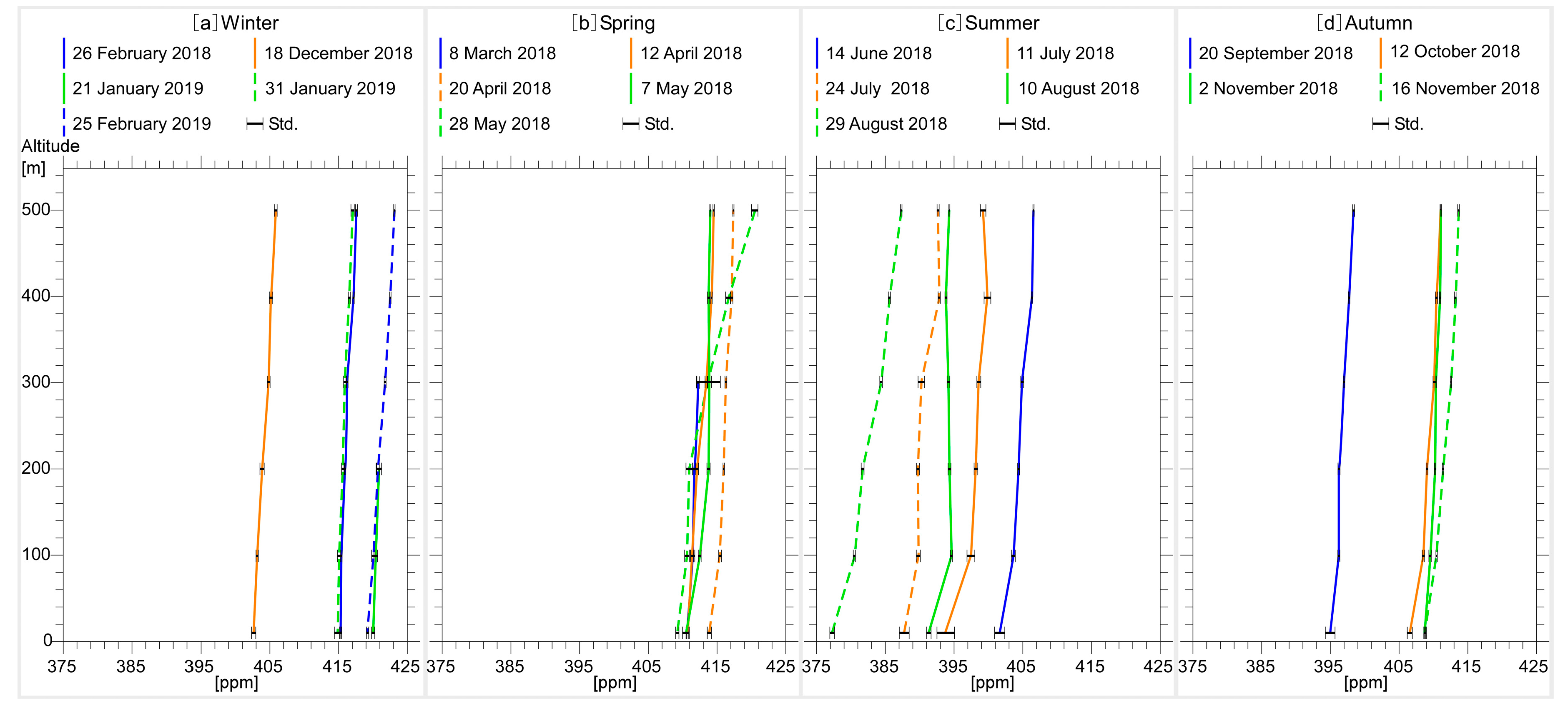
Table A3. CO₂ concentrations (mean ± standard deviation) in ppm, measured by the UAV system at each altitude during its decent from winter 2018 to winter 2019.

Altitude	26 February 2018	8 March 2018	12 April 2018	20 April 2018	7 May 2018	28 May 2018	14 June 2018
500 m	417.08 ± 0.15		414.83 ± 0.10	417.35 ± 0.08	414.17 ± 0.08	420.5 ± 0.46	406.58 ± 0.08
400 m	416.67 ± 0.10		414.55 ± 0.10	417.31 ± 0.18	413.82 ± 0.17	416.71 ± 0.38	406.26 ± 0.10
300 m	415.91 ± 0.12	412.48 ± 0.18	413.73 ± 0.21	416.43 ± 0.13	414.14 ± 0.31	413.07 ± 1.75	404.85 ± 0.20
200 m	415.53 ± 0.08	412.01 ± 0.23	412.41 ± 0.19	416.06 ± 0.10	413.79 ± 0.24	411.13 ± 0.48	404.32 ± 0.14
100 m	415.15 ± 0.10	411.60 ± 0.28	411.71 ± 0.24	415.44 ± 0.21	412.69 ± 0.21	410.89 ± 0.34	403.67 ± 0.28
10 m	414.94 ± 0.15	411.14 ± 0.15	411.01 ± 0.15	413.94 ± 0.30	410.99 ± 0.50	409.4 ± 0.24	401.64 ± 0.73
Altitude	11 July 2018	24 July 2018	10 August 2018	29 August 2018	20 September 2018	12 October 2018	2 November 2018
500 m	399.21 ± 0.40	392.51 ± 0.16	393.80 ± 0.00	387.45 ± 0.10	398.52 ± 0.15	411.09 ± 0.11	411.44 ± 0.00
400 m	399.85 ± 0.49	392.75 ± 0.17	393.39 ± 0.15	385.66 ± 0.15	397.82 ± 0.10	410.75 ± 0.15	411.12 ± 0.10
300 m	398.55 ± 0.28	390.16 ± 0.48	393.60 ± 0.19	384.38 ± 0.19	397.30 ± 0.10	410.17 ± 0.18	410.42 ± 0.10
200 m	398.00 ± 0.42	389.65 ± 0.21	393.78 ± 0.21	381.71 ± 0.21	396.37 ± 0.14	409.08 ± 0.11	410.22 ± 0.10
100 m	397.56 ± 0.56	389.68 ± 0.29	394.05 ± 0.16	380.46 ± 0.16	396.31 ± 0.14	408.61 ± 0.17	409.71 ± 0.17
10 m	393.76 ± 1.29	387.68 ± 0.72	390.70 ± 0.34	377.25 ± 0.34	395.23 ± 0.71	406.94 ± 0.37	408.79 ± 0.08
Altitude	16 November 2018	18 December 2018	21 January 2019	31 January 2019	25 February 2019
500 m	413.81 ± 0.11	405.46 ± 0.21		416.76 ± 0.25	422.37 ± 0.10
400 m	413.20 ± 0.11	404.90 ± 0.25		416.54 ± 0.17	421.72 ± 0.11
300 m	412.67 ± 0.08	404.49 ± 0.21		416.15 ± 0.18	421.16 ± 0.14
200 m	411.42 ± 0.10	403.69 ± 0.31	420.28 ± 0.39	415.70 ± 0.18	419.97 ± 0.19
100 m	410.55 ± 0.10	402.96 ± 0.17	419.72 ± 0.27	415.31 ± 0.25	419.44 ± 0.24
10 m	409.04 ± 0.20	402.23 ± 0.31	419.19 ± 0.23	414.89 ± 0.47	418.69 ± 0.17

Table A4. CO₂ concentrations (mean ± standard deviation) in ppm, measured by the UAV system at each altitude during its ascent from winter 2018 to winter 2019.

Altitude	26 February 2018	8 March 2018	12 April 2018	20 April 2018	7 May 2018	28 May 2018	14 June 2018
500 m							406.36 ± 0.14
400 m							404.86 ± 0.28
300 m							404.56 ± 0.23
200 m							405.00 ± 0.11
100 m							404.47 ± 0.17
10 m							403.06 ± 0.38
Altitude	11 July 2018	24 July 2018	10 August 2018	29 August 2018	20 September 2018	12 October 2018	2 November 2018
500 m		392.99 ± 0.49	394.89 ± 0.24	387.23 ± 1.48	398.38 ± 0.17	411.14 ± 0.19	411.14 ± 0.10
400 m		390.03 ± 0.51	394.41 ± 0.11	382.80 ± 0.25	398.29 ± 0.11	410.90 ± 0.11	410.89 ± 0.07
300 m		390.89 ± 0.25	394.08 ± 0.31	381.76 ± 0.47	397.80 ± 0.08	410.17 ± 0.24	410.23 ± 0.09
200 m		389.72 ± 0.17	393.50 ± 0.31	382.92 ± 0.55	396.75 ± 0.12	409.53 ± 0.22	409.80 ± 0.10
100 m		389.38 ± 0.13	392.75 ± 0.62	379.07 ± 0.42	396.72 ± 0.18	409.39 ± 0.18	409.47 ± 0.09
10 m		388.82 ± 0.47	390.97 ± 1.07	374.29 ± 1.39	395.76 ± 0.63	407.40 ± 0.41	408.67 ± 0.33
Altitude	16 November 2018	18 December 2018	21 January 2019	31 January 2019	25 February 2019
500 m	413.74 ± 0.08	412.13 ± 0.12		417.54 ± 0.24	422.58 ± 0.23
400 m	413.37 ± 0.24	411.74 ± 0.28		417.25 ± 0.50	421.63 ± 0.22
300 m	412.87 ± 0.15	411.56 ± 0.16		416.86 ± 0.33	421.22 ± 0.49
200 m	411.19 ± 0.11	410.71 ± 0.23	418.17 ± 0.40	416.34 ± 0.24	420.33 ± 0.22
100 m	410.89 ± 0.13	410.05 ± 0.15	417.59 ± 0.29	415.83 ± 0.12	419.58 ± 0.23
10 m	410.58 ± 0.11	409.36 ± 0.15	417.04 ± 0.24	415.70 ± 0.26	419.35 ± 0.19

Figure A1. Comparison of CO₂ concentrations measured during the UAV’s descent (Table A3) with those measured during its ascent (Table A4).

Table A5. Major specifications of the Lithium-ion battery.

Model Name	GANGAN GT5
Rated Output	DC 14.8 V, 10400 mAh
Temperature range	0~+40 °C
Size (W, H, D)	156 × 99 × 45 mm
Weight	0.95 kg

Table A6. CO₂ concentrations (mean ± standard deviation) in ppm measured by the UAV system during propeller stopping and rotation times on the surface of measuring site.

Observation Period	1st Time	2nd Time
During propeller stopping	385.58 ± 0.31	388.16 ± 0.87
During propeller rotating	384.54 ± 0.36	387.03 ± 0.87

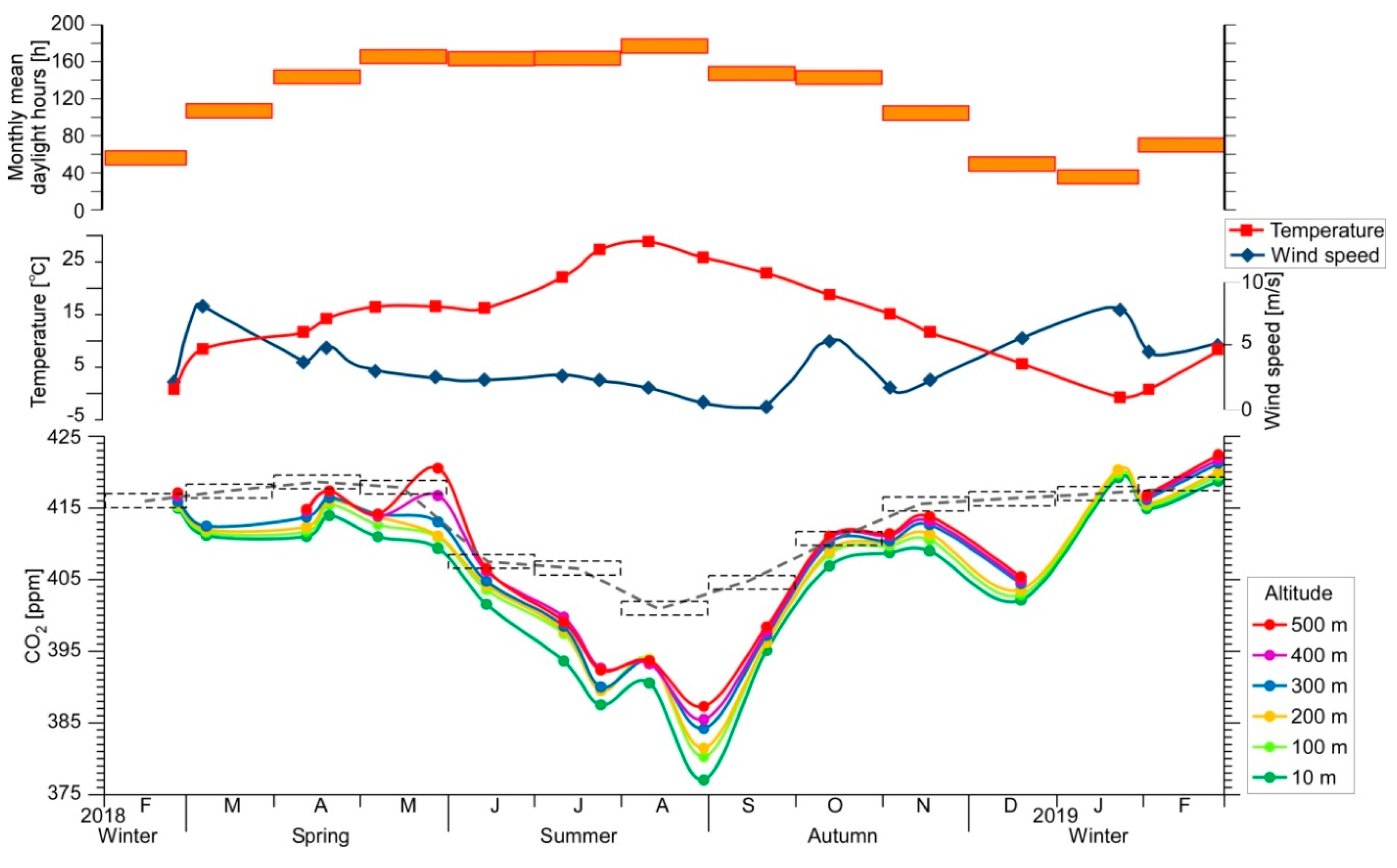
Table A7. General annual farm work schedule and corresponding rice life stages in farmlands of central Akita Prefecture (based on [48,49]) and simulated CO₂ concentrations (from [33]).

Month	October–November (Previous Year)	March	Early April–Mid April	May	Late June	July	August	Early September	Late September–October	October	October–November
Farm works	Tilling rice fields	Preparation for raising seedling	Plowing fields	Rice sowing and planting	Water management in rice fields	Water management in rice fields	Water management in rice fields	Pest control	Rice reaping and threshing	Rice drying, and hulling	Tilling rice fields
Farm works			Water management in rice fields	Water management in rice fields
Life stage of rice			Rice seed	Emergence of seedling	Rice growth stage	Rice growth stage	Rice growth stage	Maturation stage of panicles
Life stage of rice			Rice seed	Emergence of seedling		Panicle formation stage	Heading stage	Maturation stage of panicles
Surface CO₂ concentration (ppm)		415.4	416.6	415.9	405.6	404.6	398.7	402.8	408.8		413.6

References

Keeling, C.D.; Bacastow, R.B.; Bainbridge, A.E.; Ekdahl, C.A.; Guenther, P.R.; Waterman, L.S.; Chin, J.F.S. Atmospheric carbon dioxide variations at Mauna Loa Observatory, Hawaii. Tellus 1976, 28, 538–551. [Google Scholar] [Green Version]
Kawamura, K.; Parrenin, K.; Lisiecki, L.; Uemura, R.; Vimeux, F.; Severinghaus, J.P.; Hutterli, M.A.; Nakazawa, T.; Aoki, S.; Jouzel, J.; et al. Northern Hemisphere forcing of climatic cycles in Antarctica over the past 360,000 years. Nature 2007, 448, 912–916. [Google Scholar] [CrossRef] [PubMed]
WMO. WMO Greenhouse Gas Bulletin, The State of Greenhouse Gases in the Atmosphere Based on Global Observations through 2015, No. 12. World Meteorological Organization, 2016. Available online: http://www.wmo.int/pages/prog/arep/gaw/ghg/ghgbull06_en.html (accessed on 1 March 2019).
Schlesinger, W.H. Carbon balance in terrestrial detritus. Annu. Rev. Ecol. Syst. 1977, 8, 1–81. [Google Scholar] [CrossRef]
He, M.; Sun, Y.; Han, B. Green carbon science. Green carbon science: Scientific basis for integrating carbon resource processing, utilization, and recycling. Angew. Chem. Int. Ed. 2013, 52, 9620–9633. [Google Scholar] [CrossRef] [PubMed]
Crevoisier, C.; Clerbaux, C.; Guidard, V.; Phulpin, T.; Armante, R.; Barret, B.; Camy-Peyret, C.; Chaboureau, J.P.; Coheur, P.F.; Crépeau, L.; et al. Towards IASI-New Generation (IASI-NG): Impact of improved spectral resolution and radiometric noise on the retrieval of thermodynamic, chemistry and climate variables. Atmos. Meas. Tech. 2014, 7, 4367–4385. [Google Scholar] [CrossRef]
Crevoisier, C.; Heilliette, S.; Chédin, A.; Serrar, S.; Armante, R.; Scott, N.A. Midtropospheric CO₂ concentration retrieval from AIRS observations in the tropics. Geophys. Res. Lett. 2004, 31, L17106. [Google Scholar] [CrossRef]
Kuze, A.; Suto, H.; Nakajima, M.; Hamazaki, T. Thermal and near infrared sensor for carbon observation Fourier-transform spectrometer on the Greenhouse Gases Observing Satellite for greenhouse gases monitoring. Appl. Opt. 2009, 48, 6716–6733. [Google Scholar] [CrossRef] [PubMed]
Wunch, D.; Wennberg, P.O.; Osterman, G.; Fisher, B.; Naylor, B.; Roehl, C.M.; O’Dell, C.; Mandrake, L.; Viatte, C.; Kiel, M.; et al. Comparisons of the Orbiting Carbon Observatory-2 (OCO-2) XCO₂ measurements with TCCON. Atmos. Meas. Tech. 2017, 10, 2209–2238. [Google Scholar] [CrossRef]
Inoue, H.Y.; Matsueda, H. Measurements of atmospheric CO₂ from a meteorological tower in Tsukuba, Japan. Tellus 2001, 53, 205–219. [Google Scholar] [CrossRef]
Sasakawa, M.; Machida, T.; Tsuda, M.; Arshinov, M.; Davydov, D.; Fofonov, A.; Krasnov, O. Aircraft and tower measurement of CO₂ concentration in the planetary boundary layer and the lower free troposphere over southern taiga in West Siberia: Long-term records from 2002 to 2011. J. Geophys. Res. Atmos. 2013, 118, 9489–9498. [Google Scholar] [CrossRef]
Machida, T.; Kita, K.; Kondo, Y.; Blake, D.; Kawakami, S.; Inoue, G.; Ogawa, T. Vertical and meridional distributions of the atmospheric CO₂ mixing ratio between northern midlatitudes and southern subtropics. J. Geophys. Res. 2002, 108. [Google Scholar] [CrossRef]
Machida, T.; Matsueda, H.; Sawa, Y.; Nakagawa, Y.; Hirotani, K.; Kondo, N.; Goto, K.; Nakazawa, T.; Ishikawa, K.; Ogawa, T. Worldwide measurements of atmospheric CO₂ and other trace gas species using commercial airlines. J. Atmos. Ocean. Technol. 2008, 25, 1744–1754. [Google Scholar] [CrossRef]
Inoue, M.; Morino, I.; Uchino, O.; Miyamoto, Y.; Yoshida, Y.; Yokota, T.; Machida, T.; Sawa, Y.; Matsueda, H. Validation of XCO₂ derived from SWIR spectra of GOSAT TANSO-FTS with aircraft measurement data. Atmos. Chem. Phys. 2013, 13, 9771–9788. [Google Scholar] [CrossRef]
Nakazawa, T.; Machida, T.; Sugawara, S.; Murayama, S.; Hashida, G.; Morimoto, S.; Honda, H.; Itoh, T. Measurements of the Stratospheric Carbon Dioxide Concentration over Japan Using a Balloon-Borne Cryogenic Sampler. Geophys. Res. Lett. 1995, 22, 1229–1232. [Google Scholar] [CrossRef]
Inai, Y.; Aoki, S.; Honda, H.; Furutani, H.; Matsumi, Y.; Ouchi, M.; Sugawara, S.; Hasebe, F.; Uematsu, M.; Fujiwara, M. Balloon-borne tropospheric CO₂ observations over the equatorial eastern and western Pacific. Atmos. Environ. 2018, 184, 24–36. [Google Scholar] [CrossRef]
Jat, P.; Serre, M.L. Bayesian Maximum Entropy space/time estimation of surface water chloride in Maryland using river distances. Environ. Pollut. 2016, 219, 1148–1155. [Google Scholar] [CrossRef] [PubMed] [Green Version]
Jat, P.; Serre, M.L. A novel geostatistical approach combining Euclidean and gradual-flow covariance models to estimate fecal coliform along the Haw and Deep rivers in North Carolina. Stoch. Environ. Res. Risk Assess. 2018, 32, 1–13. [Google Scholar] [CrossRef]
Karion, A.; Sweeney, C.; Tans, P.; Newberger, T. AirCore an innovative atmospheric sampling system. J. Atmos. Ocean. Technol. 2010, 27, 1839–1853. [Google Scholar] [CrossRef]
Villa, T.F.; Jayaratne, E.R.; Gonzalez, L.F.; Morawska, L. Determination of the vertical profile of particle number concentration adjacent to a motorway using an unmanned aerial vehicle. Environ. Pollut. 2017, 230, 134–142. [Google Scholar] [CrossRef] [Green Version]
Andersen, T.; Scheeren, B.; Peters, W.; Chen, H. A UAV-Based Active AirCore System for Measurements of Greenhouse Gases. Atmos. Meas. Tech. 2018, 11, 2683–2699. [Google Scholar] [CrossRef]
Chang, C.C.; Chang, C.Y.; Wang, J.L.; Lin, M.R.; OuYang, C.F.; Pan, H.H.; Chen, Y.C. A study of atmospheric mixing of trace gases by aerial sampling with a multi-rotor drone. Atmos. Environ. 2018, 184, 254–261. [Google Scholar] [CrossRef]
Villa, T.F.; Brown, R.A.; Jayaratne, E.R.; Gonzalez, L.F.; Morawska, L.; Ristovski, Z.D. Characterization of the particle emission from a ship operating at sea using an unmanned aerial vehicle. Atmos. Meas. Tech. 2019, 12, 691–702. [Google Scholar] [CrossRef]
Schuyler, T.J.; Guzman, M.I. Unmanned Aerial Systems for Monitoring Trace Tropospheric Gases. Atmosphere 2017, 8, 206. [Google Scholar] [CrossRef]
Mamali, D.; Marinou, E.; Sciare, J.; Pikridas, M.; Kokkalis, P.; Kottas, M.; Binietoglou, I.; Tsekeri, A.; Keleshis, C.; Engelmann, R.; et al. Vertical profiles of aerosol mass concentration derived by unmanned airborne in situ and remote sensing instruments during dust events. Atmos. Meas. Tech. 2018, 11, 2897–2910. [Google Scholar] [CrossRef] [Green Version]
Schuyler, T.J.; Gohari, S.M.I.; Pundsack, G.; Berchoff, D.; Guzman, M.I. Using a Balloon-Launched Unmanned Glider to Validate Real-Time WRF Modeling. Sensors 2019, 19, 1914. [Google Scholar] [CrossRef] [PubMed]
Barbieri, L.; Kral, S.T.; Bailey, S.C.C.; Frazier, A.E.; Jacob, J.D.; Reuder, J.; Brus, D.; Chilson, P.B.; Crick, C.; Detweiler, C.; et al. Intercomparison of Small Unmanned Aircraft System (sUAS) Measurements for Atmospheric Science during the LAPSE-RATE Campaign. Sensors 2019, 19, 2179. [Google Scholar] [CrossRef] [PubMed]
Madokoro, H.; Inoue, M.; Nagayoshi, T.; Chiba, T.; Haga, Y.; Kiguchi, O.; Sato, K. Prototype development of drone system used for in-situ measurement of CO₂ vertical profile and its preliminary flight test. Trans. Soc. Instrum. Control Eng. (In Japanese with English abstract) (submitted).
Inoue, M.; Haga, Y.; Nagayoshi, T.; Madokoro, H.; Takakai, F.; Kiguchi, O.; Morino, I. Measurement of atmospheric carbon dioxide using unmanned aerial vehicle for profiling vertical distribution over Akita. In Proceedings of the 14th iCACGP Quadrennial Symposium/15th IGAC Science Conference, Takamatsu, Japan, 26 September 2018; Available online: http://icacgp-igac2018.colorado.edu/melamed/Abstracts/2.060_Inoue.pdf (accessed on 30 July 2019).
Nomura, K.; Madokoro, H.; Chiba, T.; Inoue, M.; Nagayoshi, T.; Kiguchi, O.; Woo, H.; Sato, K. Operation and Maintenance of In-Situ CO₂ Measurement System Using Unmanned Aerial Vehicles. In Proceedings of the 19th International Conference on Control, Automation and Systems, Jeju, Korea, 30 October 2019. [Google Scholar]
Li, Y.; Deng, J.; Mua, C.; Xing, Z.; Dub, K. Vertical distribution of CO₂ in the atmospheric boundary layer: Characteristics and impact of meteorological variables. Atmos. Environ. 2014, 91, 110–117. [Google Scholar] [CrossRef]
Japan Meteorological Agency. AMeDAS. 2018–2019. Available online: http://www.jma.go.jp/jp/amedas/000.html (accessed on 31 January 2019).
Japan Meteorological Agency. CO2 Concentration Secular Changes by Locations (Longitude/Latitude). 2019. Available online: http://ds.data.jma.go.jp/ghg/kanshi/co2timeser/co2timeser.html (accessed on 30 April 2019).
Nakamura, T.; Maki, T.; Machida, T.; Matsueda, H.; Sawa, Y.; Niwa, Y. Improvement of Atmospheric CO₂ Inversion Analysis at JMA, A31B-0033. In Proceedings of the AGU Fall Meeting, San Francisco, CA, USA, 14–18 December 2015. [Google Scholar]
Geospatial Information Authority of Japan. Digital Map (Elevation). Available online: http://maps.gsi.go.jp/#13/39.982513/140.003071/&base=ort&ls=ort%7Crelief_free%7Cslopemap&blend=10&disp=111&lcd=slopemap&vs=c1j0h0k0l0u0t0z0r0s0f1&d=vl 2019. (accessed on 31 January 2019).
Ogura, Y. General Meteorology, 2nd ed.; University of Tokyo Press: Toyo, Japan, 2016; 320p. [Google Scholar]
Tanaka, M.; Nakazawa, T.; Aoki, S. High Quality Measurements of the Concentration of Atmospheric Carbon Dioxide. J. Meteorol. Soc. Jpn. 1983, 61, 678–685. [Google Scholar] [CrossRef] [Green Version]
Tanaka, T.; Miyamoto, Y.; Morino, I.; Machida, T.; Nagahama, T.; Sawa, Y.; Matsueda, H.; Wunch, D.; Kawakami, S.; Uchino, O. Aircraft measurements of carbon dioxide and methane for the calibration of ground-based high-resolution Fourier Transform Spectrometers and a comparison to GOSAT data measured over Tsukuba and Moshiri. Atmos. Meas. Tech. 2012, 5, 2003–2012. [Google Scholar] [CrossRef] [Green Version]
Hupp, J.R. The Importance of Water Vapor Measurements and Corrections. LI-COR, Inc. Appl. Note 2011, 129, 1–8. [Google Scholar]
Sasaki, T.; Maki, T.; Oohashi, S.; Akagi, K. Optimal sampling network and availability of data acquired at inland sites. Glob. Atmos. Watch Rep. 2003, 148, 77–79. [Google Scholar]
Maki, T.; Ikegami, M.; Fujita, T.; Hirahara, T.; Yamada, K.; Mori, K.; Takeuchi, A.; Tsutsumi, Y.; Suda, K.; Conway, T.J. New technique to analyse global distributions of CO₂ concentrations and fluxes from non-processed observational data. Tellus 2010, 62B, 797–809. [Google Scholar] [CrossRef]
Ouchi, M.; Matsumi, Y.; Nakayama, T.; Shimizu, K.; Sawada, T.; Machida, T.; Matsueda, H.; Sawa, Y.; Morino, I.; Uchino, O.; et al. Development of a balloon-borne instrument for CO₂ vertical profile observations in the troposphere. Atmos. Meas. Tech. Discuss. 2019. [Google Scholar] [CrossRef]
Tans, P.P.; Fung, I.Y.; Takahashi, T. Observational Constrains on the Global Atmospheric CO₂ Budget. Science 1990, 247, 1431–1438. [Google Scholar] [CrossRef] [PubMed]
Randerson, J.T.; Field, C.B.; Fung, I.Y.; Tans, P.P. Increases in early season ecosystem uptake explain recent changes in the seasonal cycle of atmospheric CO₂ at high northern latitudes. Geophys. Res. Lett. 1999, 26, 2765–2768. [Google Scholar] [CrossRef]
Holton, J.R. An Introduction to Dynamic Meteorology, 4th ed.; Academic Press: New York, NY, USA, 2004; 535p. [Google Scholar]
Witte, B.M.; Singler, R.F.; Bailey, S.C.C. Development of an Unmanned Aerial Vehicle for the Measurement of Turbulence in the Atmospheric Boundary Layer. Atmosphere 2017, 8, 195. [Google Scholar] [CrossRef]
Rautenberg, A.; Graf, M.S.; Wildmann, N.; Platis, A.; Bange, J. Reviewing Wind Measurement Approaches for Fixed-Wing Unmanned Aircraft. Atmosphere 2018, 9, 422. [Google Scholar] [CrossRef]
Akita Komachi Net. Akita Komachi Net HP. Available online: http://shop.akitakomachi.net/?mode=f7 2018 (accessed on 31 January 2019).
Ogata agricultural cooperative association. Agricultural Data (Eino-shiryo); Ogata Agricultural Cooperative Association: Ogata Village, Japan, 2018; 89p. [Google Scholar]
Saito, M.; Miyata, A.; Nagai, H.; Yamada, T. Seasonal variation of carbon dioxide exchange in rice paddy field in Japan. Agric. For. Meteorol. 2005, 135, 93–109. [Google Scholar] [CrossRef]
Geospatial Information Authority of Japan. Control Point Survey and Geodetic Observation Results. Available online: https://sokuseikagis1.gsi.go.jp/index.aspx#14/40.014271/139.961228/&base=std&ls=std&disp=1&vs=c1f0 (accessed on 31 January 2019).

Figure 1. Map showing (a) location of Akita Prefecture, Japan and (b) the observation area in Ogata Village *. (c) Photograph of bird’s-eye view around Ogata Village area taken in October 2018. (*) The map based on the aerial photograph, elevation chart map by color and slope gradation map created by Geospatial Information Authority of Japan [35].

Figure 2. Change of CO₂ concentration on the ground surface at Ogata (40° N, 140° E) during the last 30 years calculated by Global Spectral Atmosphere Model-Transport Model (GSAM-TM) [33].

Figure 3. (a) Photograph of the CO₂ measuring system. (b) Whole structure of the measurement system.

Figure 4. (a) Schematic diagram of the CO₂ measurement system and (b) measured concentrations of a CO₂ standard gas (concentration 348.57 ppm) after NDIR calibration against the two CO₂ standard gases and an N₂ standard gas. The battery specifications are given in Table A5. The safe excitation voltage of the LI840-A NDIR is 10–30 V; thus, this 14.8-V battery is within tolerance.

Figure 5. Vertical profiles of CO₂ from 10 m to 500 m elevation. (a) Winter, (b) spring, (c) summer, and (d) autumn. The dots are used to show the mean CO₂ concentration during the 30-s measurement period at each altitude, and the error bars indicate standard deviations.

Figure 6. Monthly mean daylight hours at Ogata (40°0.0’ N, 139°57.0’ E) (top), air temperature at 1.5 m altitude and wind speed at 10 m altitude at Ogata (middle), and seasonal variations of CO₂ concentrations at each measurement altitude (bottom) from winter 2018 to winter 2019. The dashed line shows secular CO₂ concentration changes in the ground surface at Ogata (40° N, 140° E) based on the simulation by GSAM-TM [33].

Table 1. Major specifications of the non-dispersive infrared (NDIR) analyzer.

Model Name	LI-840A
Measurement range	0–20,000 ppm
Input voltage DC	12–30 V
Power consumption	3.6 W
Temperature range	−20~+45 °C
Size (W, D, H)	222 × 152 × 76 mm
Weight	1.0 kg

Table 2. Major specifications of the unmanned aerial vehicle (UAV).

Model Name	Matrice600
Body size (W, D, H)	1668 × 1518 × 759 mm
Weight	9.1 kg (When TB47S batteries using)
Payload	6.0 kg (max)
Rising speed	5.0 m/s (max)
Dropping speed	3.0 m/s (max)
Horizontal flight speed	18.0 m/s (max)
Signal transmission range	3.5 km (max)

Table 3. Surface temperature at 1.5 m altitude, wind direction and speed at 10 m altitude, and sunshine duration (see text for details) based on hourly data at Ogata on each survey date from February 2018 to February 2019.

Date	Weather	Surface Temperature (°C)	Surface Wind Direction	Surface Wind Speed (m/s)	Surface Sunshine Duration (h/h)
26 February 2018	Cloudy	0.9	NW	2.3	0.2
8 March 2018	Cloudy	8.5	SE	8.0	0.1
12 April 2018	Sunny	11.7	WNW	3.9	1.0
20 April 2018	Sunny	14.2	SSW	4.8	0.6
7 May 2018	Sunny	16.4	WNW	3.2	0.3
28 May 2018	Sunny	16.5	NW	2.9	1.0
14 June 2018	Cloudy	16.2	NW	2.7	0.4
11 July 2018	Cloudy	22.0	NW	3.0	0.1
24 July 2018	Sunny	27.2	NNW	2.5	1.0
10 August 2018	Cloudy	28.7	WNW	2.1	0.7
29 August 2018	Cloudy	25.7	ESE	1.1	0.0
20 September 2018	Cloudy	22.8	S	0.7	0.1
12 October 2018	Sunny	18.7	NW	5.4	0.8
2 November 2018	Sunny	15.1	NW	2.0	0.4
16 November 2018	Cloudy	11.7	SSE	2.6	0.3
18 December 2018	Sunny	5.7	WNW	5.6	0.5
21 January 2019	Cloudy	-0.6	WNW	7.8	0.1
31 January 2019	Cloudy	0.9	WNW	4.7	0.0
25 February 2019	Sunny	8.4	WNW	5.2	0.6

© 2019 by the authors. Licensee MDPI, Basel, Switzerland. This article is an open access article distributed under the terms and conditions of the Creative Commons Attribution (CC BY) license (http://creativecommons.org/licenses/by/4.0/).

Share and Cite

MDPI and ACS Style

Chiba, T.; Haga, Y.; Inoue, M.; Kiguchi, O.; Nagayoshi, T.; Madokoro, H.; Morino, I. Measuring Regional Atmospheric CO₂ Concentrations in the Lower Troposphere with a Non-Dispersive Infrared Analyzer Mounted on a UAV, Ogata Village, Akita, Japan. Atmosphere 2019, 10, 487. https://0-doi-org.brum.beds.ac.uk/10.3390/atmos10090487

AMA Style

Chiba T, Haga Y, Inoue M, Kiguchi O, Nagayoshi T, Madokoro H, Morino I. Measuring Regional Atmospheric CO₂ Concentrations in the Lower Troposphere with a Non-Dispersive Infrared Analyzer Mounted on a UAV, Ogata Village, Akita, Japan. Atmosphere. 2019; 10(9):487. https://0-doi-org.brum.beds.ac.uk/10.3390/atmos10090487

Chicago/Turabian Style

Chiba, Takashi, Yumi Haga, Makoto Inoue, Osamu Kiguchi, Takeshi Nagayoshi, Hirokazu Madokoro, and Isamu Morino. 2019. "Measuring Regional Atmospheric CO₂ Concentrations in the Lower Troposphere with a Non-Dispersive Infrared Analyzer Mounted on a UAV, Ogata Village, Akita, Japan" Atmosphere 10, no. 9: 487. https://0-doi-org.brum.beds.ac.uk/10.3390/atmos10090487

Note that from the first issue of 2016, this journal uses article numbers instead of page numbers. See further details here.

Article Menu

Measuring Regional Atmospheric CO₂ Concentrations in the Lower Troposphere with a Non-Dispersive Infrared Analyzer Mounted on a UAV, Ogata Village, Akita, Japan

Abstract

1. Introduction