Vertical Profiles of Ozone Concentration Collected by an Unmanned Aerial Vehicle and the Mixing of the Nighttime Boundary Layer over an Amazonian Urban Area

 ,
,  , , and
Abstract
:1. Introduction
2. Methodology
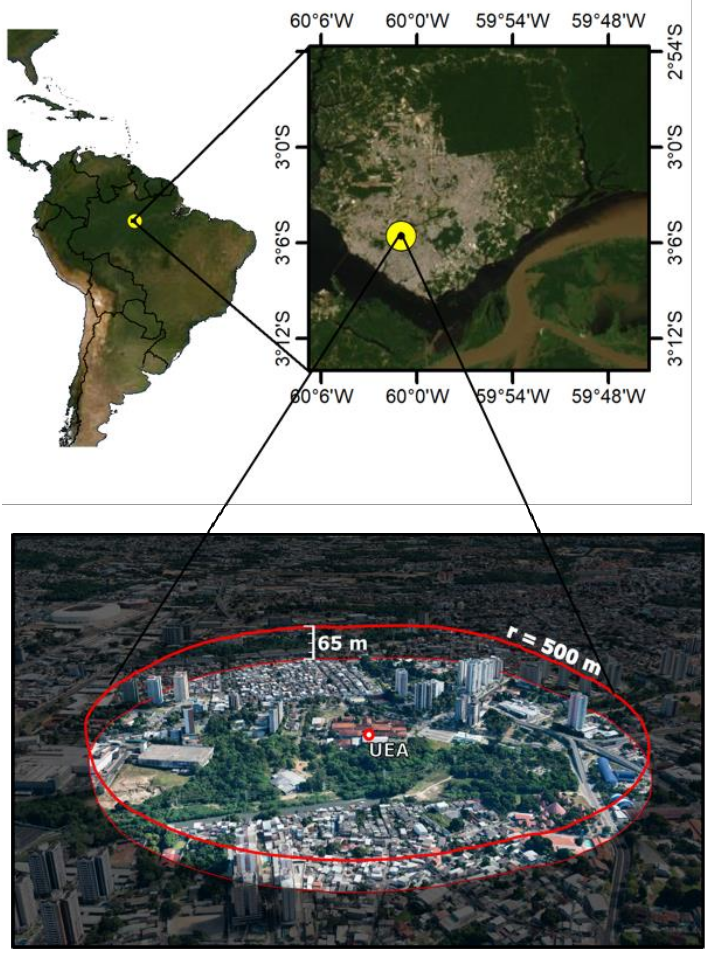
2.1. Location
2.2. Flight Platform and Instrumentation
2.3. UAV Flights
2.4. Data Analysis
3. Results and Discussion
4. Conclusions
Supplementary Materials
Author Contributions
Funding
Acknowledgments
Conflicts of Interest
References and Note
- Stull, R.B. An Introduction to Boundary Layer Meteorology; Kluwer Academic Publishers: Dordrecht, The Netherlands, 1988. [Google Scholar]
- Freire, L.S.; Gerken, T.; Ruiz-Plancarte, J.; Wei, D.; Fuentes, J.D.; Katul, G.G.; Dias, N.L.; Acevedo, O.C.; Chamecki, M. Turbulent mixing and removal of ozone within an Amazon rainforest canopy. J. Geophys. Res. Atmos. 2017, 122, 2791–2811. [Google Scholar] [CrossRef]
- Steeneveld, G.-J.; Nappo, C.J.; Holtslag, A.A. Estimation of orographically induced wave drag in the stable boundary layer during the CASES-99 experimental campaign. Acta Geophys. 2009, 57, 857–881. [Google Scholar] [CrossRef]
- Newsom, R.K.; Banta, R.M. Shear-flow instability in the stable nocturnal boundary layer as observed by Doppler lidar during CASES-99. J. Atmos. Sci. 2003, 60, 16–33. [Google Scholar] [CrossRef]
- Zilitinkevich, S.S.; Esau, I.N. The effect of baroclinicity on the equilibrium depth of neutral and stable planetary boundary layers. Q. J. Royal Meteorol. Soc. 2003, 129, 3339–3356. [Google Scholar] [CrossRef]
- Aneja, V.P.; Adams, A.A.; Arya, S.P. An observational based analysis of ozone trends and production for urban areas in North Carolina. Chemosphere Global Chang. Sci. 2000, 2, 157–165. [Google Scholar] [CrossRef] [Green Version]
- Corsmeier, U.; Kalthoff, N.; Kolle, O.; Kotzian, M.; Fiedler, F. Ozone concentration jump in the stable nocturnal boundary layer during a LLJ-event. Atmos. Environ. 1997, 31, 1977–1989. [Google Scholar] [CrossRef]
- Salmond, J.A.; McKendry, I.G. Secondary ozone maxima in a very stable nocturnal boundary layer: observations from the Lower Fraser Valley, BC. Atmos. Environ. 2002, 36, 5771–5782. [Google Scholar] [CrossRef]
- Oke, T. The Heat Island of the Urban Boundary Layer: Characteristics, Causes and Effects; Springer: Dordrecht, The Netherlands, 1995; pp. 81–107. [Google Scholar]
- Santos, R.M.N. Study of the Nocturnal Boundary Layer in the Amazon. Ph.D. Thesis, National Institute of Space Research, Sao Jose dos Campos, SP, Brazil, 2005. [Google Scholar]
- Mahrt, L.; Heald, R.C.; Lenschow, D.H.; Stankov, B.B.; Troen, I.B. An observational study of the structure of the nocturnal boundary layer. Bound.-Layer Meteorol. 1979, 17, 247–264. [Google Scholar] [CrossRef]
- Mahrt, L. Vertical structure and turbulence in the very stable boundary layer. J. Atmos. Sci. 1985, 42, 2333–2349. [Google Scholar] [CrossRef]
- Finnigan, J. A note on wave-turbulence interaction and the possibility of scaling the very stable boundary layer. Bound.-Layer Meteorol. 1999, 90, 529–539. [Google Scholar] [CrossRef]
- Sun, J.; Lenschow, D.H.; Burns, S.P.; Banta, R.M.; Newsom, R.K.; Coulter, R.; Frasier, S.; Ince, T.; Nappo, C.; Balsley, B.B. Atmospheric disturbances that generate intermittent turbulence in nocturnal boundary layers. Bound.-Layer Meteorol. 2004, 110, 255–279. [Google Scholar] [CrossRef]
- Yerramilli, A.; Challa, V.S.; Dodla, V.B.R.; Dasari, H.P.; Young, J.H.; Patrick, C.; Baham, J.M.; Hughes, R.L.; Hardy, M.G.; Swanier, S.J. Simulation of surface ozone pollution in the central gulf coast region using WRF/Chem Model: Sensitivity to PBL and Land Surface Physics. Atmos. Pollut. Res. 2010, 3, 55–71. [Google Scholar] [CrossRef]
- Neves, T.T.A.T.; Fisch, G. Night limit layer on pasture area in the Amazon. Rev. Bras. Meteorol. 2011, 26, 619–628. [Google Scholar] [CrossRef]
- Banta, R.M.; Pichugina, Y.L.; Brewer, W.A. Turbulent velocity-variance profiles in the stable boundary layer generated by a nocturnal low-level jet. J. Atmos. Sci. 2006, 63, 2700–2719. [Google Scholar] [CrossRef]
- Duarte, H.F.; Leclerc, M.Y.; Zhang, G. Assessing the shear-sheltering theory applied to low-level jets in the nocturnal stable boundary layer. Theor. Appl. Climatol. 2012, 110, 359–371. [Google Scholar] [CrossRef]
- Santana, R.A.S.; Tóta, J.; Santos, R.M.N.; Vale, R.S. Stability and struture of turbulence under the influence of jets of low night levels in the Southwest Amazon. Rev. Bras. Meteorol. 2015, 30, 405–414. [Google Scholar] [CrossRef]
- Betts, A.K.; Gatti, L.V.; Cordova, A.M.; Dias, M.A.S.; Fuentes, J.D. Transport of ozone to the surface by convective downdrafts at night. J. Geophys. Res. Atmos. 2002, 107, LBA 13-11–LBA 13-16. [Google Scholar] [CrossRef]
- Gerken, T.; Wei, D.; Chase, R.J.; Fuentes, J.D.; Schumacher, C.; Machado, L.A.; Andreoli, R.V.; Chamecki, M.; de Souza, R.A.F.; Freire, L.S. Downward transport of ozone rich air and implications for atmospheric chemistry in the Amazon rainforest. Atmos. Environ. 2016, 124, 64–76. [Google Scholar] [CrossRef] [Green Version]
- Hu, X.-M.; Doughty, D.C.; Sanchez, K.J.; Joseph, E.; Fuentes, J.D. Ozone variability in the atmospheric boundary layer in Maryland and its implications for vertical transport model. Atmos. Environ. 2012, 46, 354–364. [Google Scholar] [CrossRef]
- Andreae, M.O.; Acevedo, O.C.; Araújo, A.; Artaxo, P.; Barbosa, C.G.G.; Barbosa, H.M.J.; Brito, J.; Carbone, S.; Chi, X.; Cintra, B.B.L. The Amazon Tall Tower Observatory (ATTO): overview of pilot measurements on ecosystem ecology, meteorology, trace gases, and aerosols. Atmos. Chem. Phys. 2015, 15, 10723–10776. [Google Scholar] [CrossRef] [Green Version]
- Oliveira, P.E.; Acevedo, O.C.; Sörgel, M.; Tsokankunku, A.; Wolff, S.; Araújo, A.C.; Souza, R.A.; Sá, M.O.; Manzi, A.O.; Andreae, M.O. Nighttime wind and scalar variability within and above an Amazonian canopy. Atmos. Chem. Phys. 2018, 18, 3083–3099. [Google Scholar] [CrossRef] [Green Version]
- Seibert, P.; Beyrich, F.; Gryning, S.-E.; Joffre, S.; Rasmussen, A.; Tercier, P. Review and intercomparison of operational methods for the determination of the mixing height. Atmos. Environ. 2000, 34, 1001–1027. [Google Scholar] [CrossRef]
- Fisch, G. Amazonian boundary layer: Observations and modeling aspects. Rev. Bras. Geof. 1999, 17, 85–86. [Google Scholar] [CrossRef]
- Sugiyama, G.; Nasstrom, J.S. Methods for Determining the Height of the Atmospheric Boundary Layer; Lawrence Livermore National Laboratory: Springfield, VA, USA, 1999; p. 11. [Google Scholar]
- Cros, B.; Fontan, J.; Minga, A.; Helas, G.; Nganga, D.; Delmas, R.; Chapuis, A.; Benech, B.; Andreae, M. Vertical profiles of ozone between 0 - 400 meters in and above the African Equatorial Forest. J. Geophys. Res. 1992, 97, 12877–12887. [Google Scholar] [CrossRef]
- Maeda, E.E.; Ma, X.; Wagner, F.H.; Kim, H.; Oki, T.; Eamus, D.; Huete, A. Evapotranspiration seasonality across the Amazon Basin. Earth Syst. Dynam 2017, 8, 439–454. [Google Scholar] [CrossRef] [Green Version]
- Behrendt, A.; Pal, S.; Aoshima, F.; Bender, M.; Blyth, A.; Corsmeier, U.; Cuesta, J.; Dick, G.; Dorninger, M.; Flamant, C. Observation of convection initiation processes with a suite of state-of-the-art research instruments during COPS IOP 8b. Q. J. Royal Meteorol. Soc. 2011, 137, 81–100. [Google Scholar] [CrossRef] [Green Version]
- Pal, S.; Lopez, M.; Schmidt, M.; Ramonet, M.; Gibert, F.; Xueref-Remy, I.; Ciais, P. Investigation of the atmospheric boundary layer depth variability and its impact on the 222Rn concentration at a rural site in France. J. Geophys. Res. Atmos 2015, 120, 623–643. [Google Scholar] [CrossRef]
- Gibert, F.; Schmidt, M.; Cuesta, J.; Ciais, P.; Ramonet, M.; Xueref, I.; Larmanou, E.; Flamant, P.H. Retrieval of average CO2 fluxes by combining in situ CO2 measurements and backscatter lidar information. J. Geophys. Res. Atmos. 2007, 112, D10301. [Google Scholar] [CrossRef]
- Gerbig, C.; Körner, S.; Lin, J. Vertical mixing in atmospheric tracer transport models: error characterization and propagation. Atmos. Chem. Phys. 2008, 8, 591–602. [Google Scholar] [CrossRef] [Green Version]
- Chambers, S.; Williams, A.; Crawford, J.; Griffiths, A.D.; Discussions, P. On the use of radon for quantifying the effects of atmospheric stability on urban emissions. Atmos. Chem. Phys. 2014, 14, 1175–1190. [Google Scholar] [CrossRef]
- Janssen, R.; Vilà-Guerau de Arellano, J.; Ganzeveld, L.; Kabat, P.; Jimenez, J.; Farmer, D.; Van Heerwaarden, C.; Mammarella, I. Combined effects of surface conditions, boundary layer dynamics and chemistry on diurnal SOA evolution. Atmos. Chem. Phys. 2012, 12, 6827–6843. [Google Scholar] [CrossRef] [Green Version]
- Pal, S.; Lee, T.; Phelps, S.; De Wekker, S.J.S.o.t.T.E. Impact of atmospheric boundary layer depth variability and wind reversal on the diurnal variability of aerosol concentration at a valley site. Sci. Total Environ. 2014, 496, 424–434. [Google Scholar] [CrossRef] [PubMed]
- Dang, R.; Yang, Y.; Hu, X.-M.; Wang, Z.; Zhang, S. A Review of Techniques for Diagnosing the Atmospheric Boundary Layer Height (ABLH) Using Aerosol Lidar Data. Remote Sens. 2019, 11, 1590. [Google Scholar] [CrossRef]
- BRAZIL. Establish air quality standards and other measures. National Council of Environment (CONAMA). Resolution no. 003/1990 of June 28, 1990.
- Li, X.; Liu, J.; Mauzerall, D.L.; Emmons, L.K.; Walters, S.; Horowitz, L.W.; Tao, S. Effects of trans-Eurasian transport of air pollutants on surface ozone concentrations over Western China. J. Geophys. Res. Atmos. 2014, 119, 12–338. [Google Scholar] [CrossRef]
- Tang, G.; Zhu, X.; Xin, J.; Hu, B.; Song, T.; Sun, Y.; Zhang, J.; Wang, L.; Cheng, M.; Chao, N. Modelling study of boundary-layer ozone over northern China-Part I: Ozone budget in summer. Atmos. Res. 2017, 187, 128–137. [Google Scholar] [CrossRef]
- Chen, P.; Quan, J.; Zhang, Q.; Tie, X.; Gao, Y.; Li, X.; Huang, M. Measurements of vertical and horizontal distributions of ozone over Beijing from 2007 to 2010. Atmos. Environ. 2013, 74, 37–44. [Google Scholar] [CrossRef]
- Wei, D.; Ruiz-Plancarte, J.; Freire, L.S.; Gerken, T.; Chamecki, M.; Fuentes, J.D.; Stoy, P.C.; Trowbridge, A.M.; dos Santos, R.M.N.; Acevedo, O. Relationship between canopy turbulence and vertical distribution of reactive gases in the central Amazon rainforest. Ciência e Natura 2016, 38, 543–547. [Google Scholar] [CrossRef]
- Fares, S.; McKay, M.; Holzinger, R.; Goldstein, A.H.; Meteorology, F. Ozone fluxes in a Pinus ponderosa ecosystem are dominated by non-stomatal processes: Evidence from long-term continuous measurements. Agric. For. Meteorol. 2010, 150, 420–431. [Google Scholar] [CrossRef]
- Fares, S.; Loreto, F.; Kleist, E.; Wildt, J. Stomatal uptake and stomatal deposition of ozone in isoprene and monoterpene emitting plants. Plant Biol. 2007, 9, 44–54. [Google Scholar] [CrossRef]
- Schaub, M.; Skelly, J.; Zhang, J.; Ferdinand, J.A.; Savage, J.E.; Stevenson, R.; Davis, D.D.; Steiner, K.C. Physiological and foliar symptom response in the crowns of Prunus serotina, Fraxinus americana and Acer rubrum canopy trees to ambient ozone under forest conditions. Environ. Pollut. 2005, 133, 553–567. [Google Scholar] [CrossRef]
- Karnosky, D.; Pregitzer, K.S.; Zak, D.R.; Kubiske, M.E.; Hendrey, G.; Weinstein, D.; Nosal, M.; Percy, K.J.P. Scaling ozone responses of forest trees to the ecosystem level in a changing climate. Plant Cell Environ. 2005, 28, 965–981. [Google Scholar] [CrossRef] [Green Version]
- Tjoelker, M.; Luxmoore, R.J.N.P. Soil nitrogen and chronic ozone stress influence physiology, growth and nutrient status of Pinus taeda L. and Liriodendron tulipifera L. seedlings. New Phytol. 1991, 119, 69–81. [Google Scholar] [CrossRef]
- Kurpius, M.R.; Goldstein, A.H. Gas-phase chemistry dominates O3 loss to a forest, implying a source of aerosols and hydroxyl radicals to the atmosphere. Geophys. Res. Lett. 2003, 30, 24. [Google Scholar] [CrossRef]
- Wieser, G.; Häsler, R.; Götz, B.; Koch, W.; Havranek, W.J.E.P. Role of climate, crown position, tree age and altitude in calculated ozone flux into needles of Picea abies and Pinus cembra: a synthesis. Environ. Pollut. 2000, 109, 415–422. [Google Scholar] [CrossRef]
- Paoletti, E.; De Marco, A.; Beddows, D.C.; Harrison, R.M.; Manning, W.J. Ozone levels in European and USA cities are increasing more than at rural sites, while peak values are decreasing. Environ. Pollut. 2014, 192, 295–299. [Google Scholar] [CrossRef]
- Sicard, P.; De Marco, A.; Troussier, F.; Renou, C.; Vas, N.; Paoletti, E.J.A.E. Decrease in surface ozone concentrations at Mediterranean remote sites and increase in the cities. Atmos. Environ. 2013, 79, 705–715. [Google Scholar] [CrossRef]
- IBGE. Brazilian Institute of Geography and Statistics. Available online: https://cidades.ibge.gov.br/brasil/am/manaus/panorama (accessed on 20 June 2019).
- BRAZIL. National Institute of Meteorology. Available online: http://www.inmet.gov.br/portal/index.php?r=clima/normaisClimatologicas (accessed on 5 September 2019).
- ANAC. National Civil Aviation Agency. Available online: http://www.anac.gov.br/assuntos/legislacao/legislacao-1/rbha-e-rbac/rbac/rbac-e-94-emd-00 (accessed on 2 July 2019).
- Santos, R.M.N.; Fisch, G.; Dolman, A.; Waterloo, M. Modeling of the Night Limit Layer (CLN) during the wet season in the Amazon under different development conditions. Rev. Bras. Meteorol. 2007, 22, 387–407. [Google Scholar] [CrossRef]
- Choi, W.; Faloona, I.; McKay, M.; Goldstein, A.; Baker, B.J.A.C. Estimating the atmospheric boundary layer height over sloped, forested terrain from surface spectral analysis during BEARPEX. Atmos. Chem. Phys. 2011, 11, 6837–6853. [Google Scholar] [CrossRef]
- Liebetrau, A.M. Measures of association; Sage: Newbury Park, CA, USA, 1983; Volume 32. [Google Scholar]
- Rolph, G.; Stein, A.; Stunder, B. Real-time environmental applications and display sYstem: READY. Environ. Model. Softw 2017, 95, 210–228. [Google Scholar] [CrossRef]
- NOAA (National Oceanic and Atmospheric Administration). Global Data Assimilation System (GDAS). Available online: https://www.ncdc.noaa.gov/data-access/model-data/model-datasets/global-data-assimilation-system-gdas (accessed on 6 August 2019).
- Kim, J.; Mahrt, L.J.T.A. Simple formulation of turbulent mixing in the stable free atmosphere and nocturnal boundary layer. Tellus A 1992, 44, 381–394. [Google Scholar] [CrossRef]
- Cramér, H. Mathematical methods of statistics; Princeton university press: Uppsala, Sweden, 1999; Volume 9. [Google Scholar]
- Malhi, Y.S.J.B.-L.M. The significance of the dual solutions for heat fluxes measured by the temperature fluctuation method in stable conditions. Bound.-Layer Meteorol. 1995, 74, 389–396. [Google Scholar] [CrossRef]
- Lenschow, D.H.; Li, X.S.; Zhu, C.J.; Stankov, B.B. The stably stratified boundary layer over the Great Plains. Bound. Layer Meteorol. 1988, 95–121. [Google Scholar] [CrossRef]
- Mahrt, L.; Sun, J.; Blumen, W.; Delany, T.; Oncley, S. Nocturnal Boundary-Layer Regimes. Bound.-Layer Meteorol. 1998, 88, 255–278. [Google Scholar] [CrossRef]
- Ohya, Y.; Neff, D.E.; Meroney, R.N. Turbulence structure in a stratified boundary layer under stable conditions. Bound.-Layer Meteorol. 1997, 83, 139–162. [Google Scholar] [CrossRef]
- Smedman, A.-S. Observations of a multi-level turbulence structure in a very stable atmospheric boundary layer. Bound.-Layer Meteorol. 1988, 44, 231–253. [Google Scholar] [CrossRef]
- Tombrou, M.; Founda, D.; Boucouvala, D. Nocturnal boundary layer height prediction from surface routine meteorological data. Meteorl. Atmos. Phys. 1998, 68, 177–186. [Google Scholar] [CrossRef]
- Betts, A.; Fisch, G.; Von Randow, C.; Silva Dias, M.; Cohen, J.; Da Silva, R.; Fitzjarrald, D. The Amazonian boundary layer and mesoscale circulations. In Amazonia and Global Change; American Geophysical Union: Washington, DC, USA, 2009. [Google Scholar] [CrossRef]
- Fisch, G.; Tota, J.; Machado, L.; Dias, M.S.; Lyra, R.d.F.; Nobre, C.; Dolman, A.; Gash, J. The convective boundary layer over pasture and forest in Amazonia. Theor. Appl. Climatol 2004, 78, 47–59. [Google Scholar] [CrossRef] [Green Version]
- Dupont, E.; Menut, L.; Carissimo, B.; Pelon, J.; Flamant, P.J.A.E. Comparison between the atmospheric boundary layer in Paris and its rural suburbs during the ECLAP experiment. Atmos. Environ. 1999, 33, 979–994. [Google Scholar] [CrossRef]
- Souza, D.O.; Alvalá, R.C.S. Observational evidence of the urban heat island of Manaus City, Brazil. Meteorol. Appl. 2014, 21, 186–193. [Google Scholar] [CrossRef]
- Arya, P.S. Introduction to Micrometeorology; Academic Press: San Diego, CA, USA, 2001; Volume 79. [Google Scholar]
- Soltani, A.; Sharifi, E. Daily variation of urban heat island effect and its correlations to urban greenery: A case study of Adelaide. Front. Archit. Res. 2017, 6, 529–538. [Google Scholar] [CrossRef]
- Oke, T.R. The urban energy balance. Prog. Phys. Geogr. 1988, 12, 471–508. [Google Scholar] [CrossRef]
- Balsley, B.B.; Jensen, M.L.; Frehlich, R.G. The use of state-of-the-art kites for profiling the lower atmosphere. Bound.-Layer Meteorol. 1998, 87, 1–25. [Google Scholar] [CrossRef]


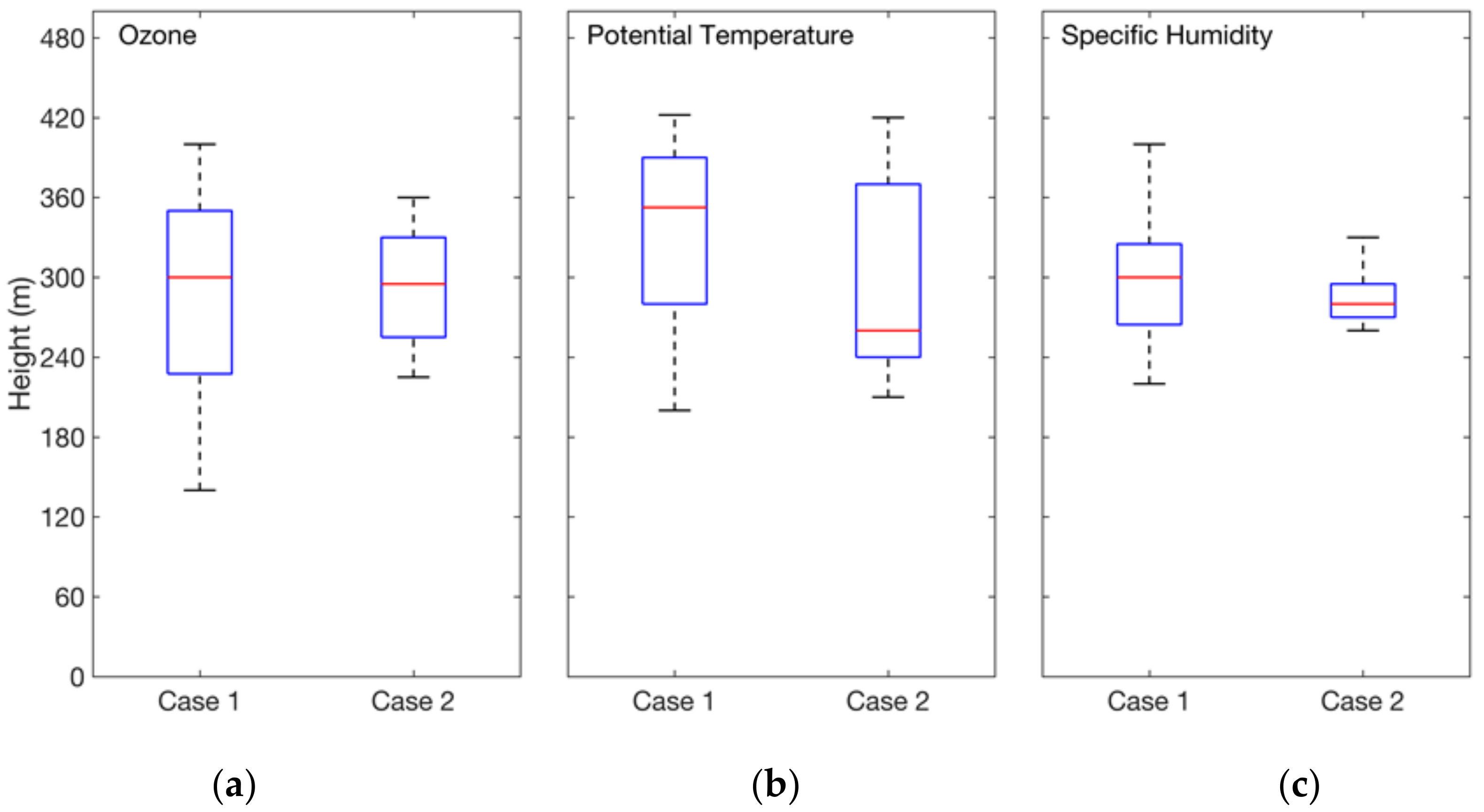
| Case | Count (N) | Percentage | Median of NBL Height (m) | Quartiles of NBL Height (m) |
|---|---|---|---|---|
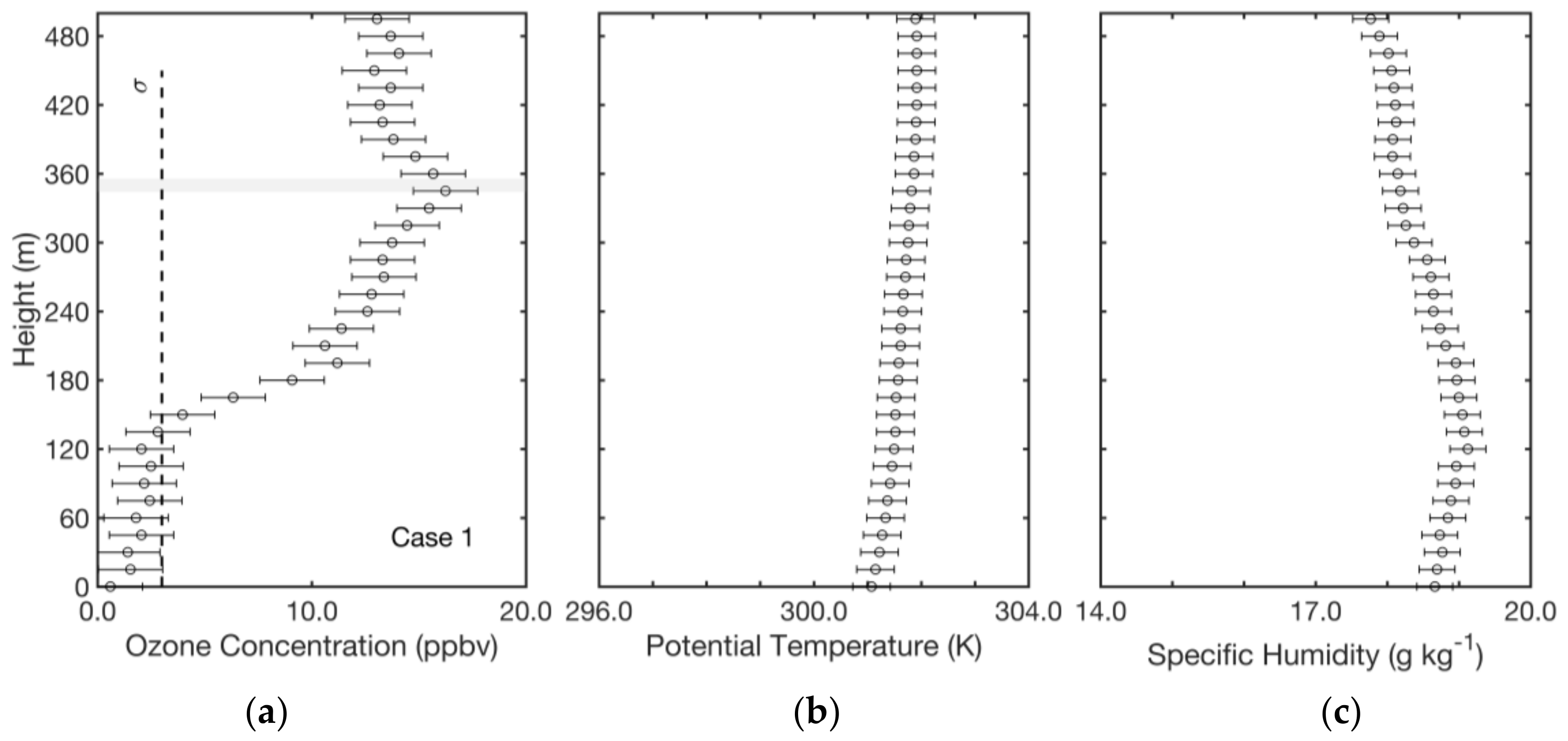
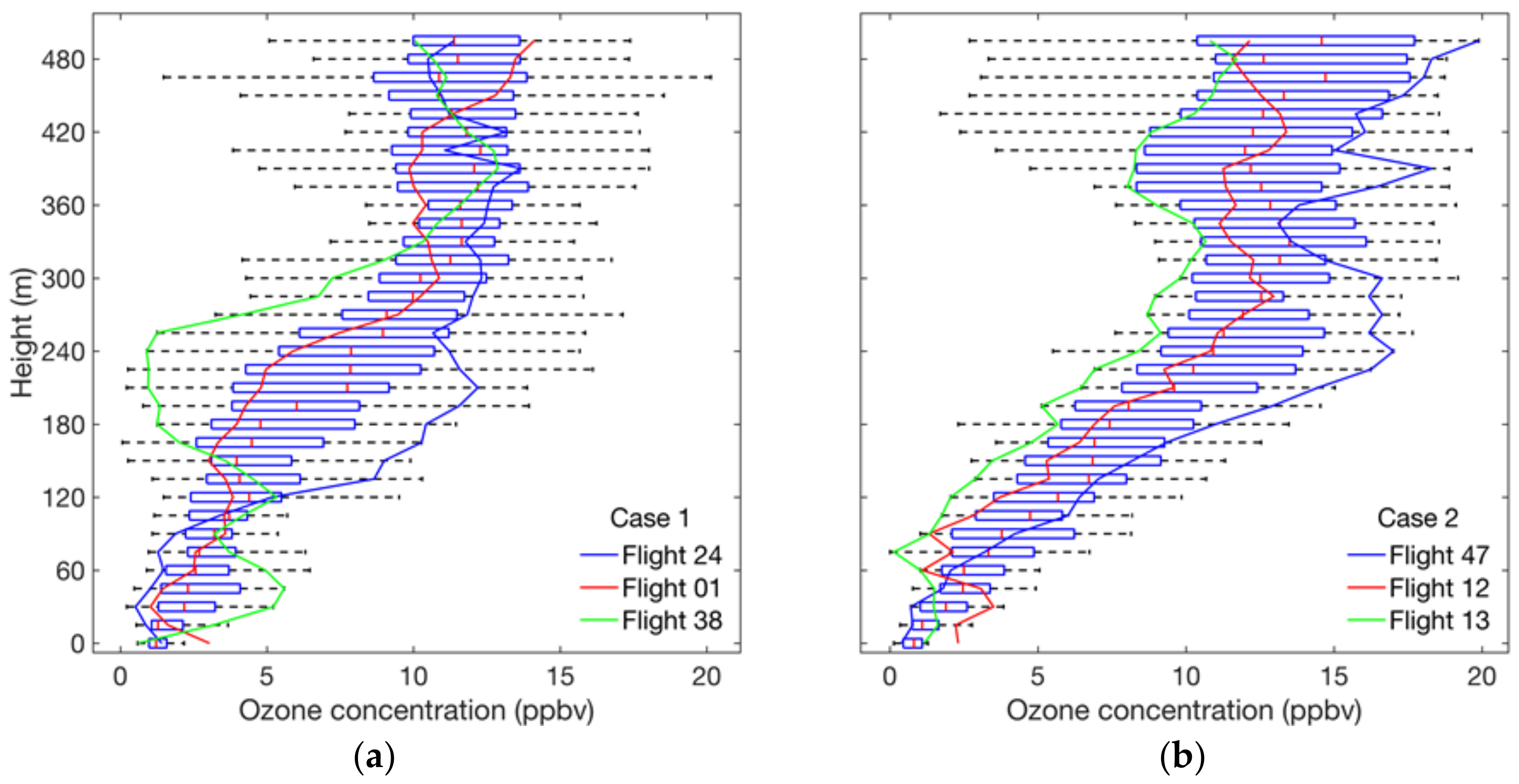
| 1: Stratified atmosphere | 23 | 40% | 300 | 230 and 350 |
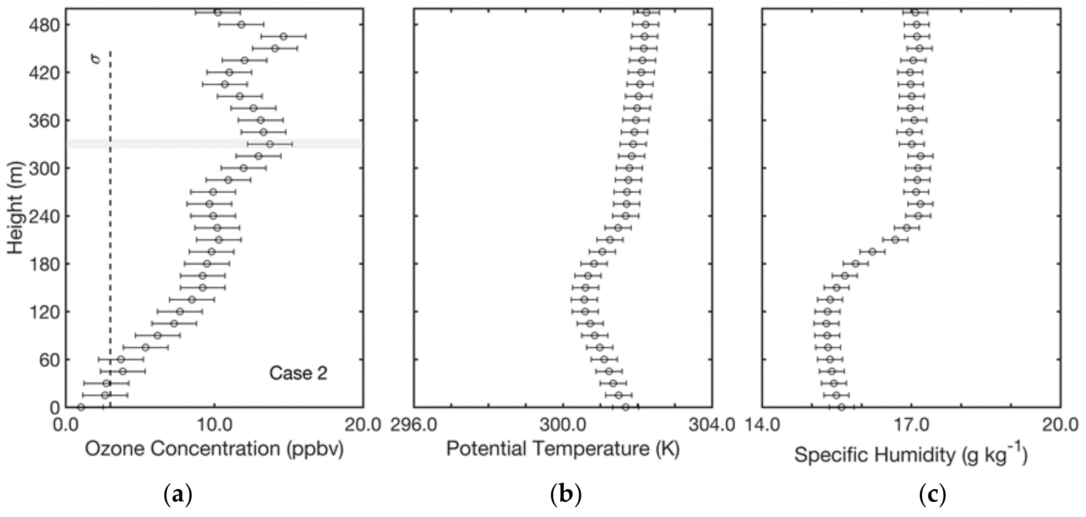
| 2: Turbulent atmosphere | 16 | 28% | 290 | 255 and 330 |
| 3: Complex atmosphere | 18 | 32% | N/A | N/A |
© 2019 by the authors. Licensee MDPI, Basel, Switzerland. This article is an open access article distributed under the terms and conditions of the Creative Commons Attribution (CC BY) license (http://creativecommons.org/licenses/by/4.0/).
Share and Cite
Guimarães, P.; Ye, J.; Batista, C.; Barbosa, R.; Ribeiro, I.; Medeiros, A.; Souza, R.; Martin, S.T. Vertical Profiles of Ozone Concentration Collected by an Unmanned Aerial Vehicle and the Mixing of the Nighttime Boundary Layer over an Amazonian Urban Area. Atmosphere 2019, 10, 599. https://0-doi-org.brum.beds.ac.uk/10.3390/atmos10100599
Guimarães P, Ye J, Batista C, Barbosa R, Ribeiro I, Medeiros A, Souza R, Martin ST. Vertical Profiles of Ozone Concentration Collected by an Unmanned Aerial Vehicle and the Mixing of the Nighttime Boundary Layer over an Amazonian Urban Area. Atmosphere. 2019; 10(10):599. https://0-doi-org.brum.beds.ac.uk/10.3390/atmos10100599
Chicago/Turabian StyleGuimarães, Patrícia, Jianhuai Ye, Carla Batista, Rafael Barbosa, Igor Ribeiro, Adan Medeiros, Rodrigo Souza, and Scot T. Martin. 2019. "Vertical Profiles of Ozone Concentration Collected by an Unmanned Aerial Vehicle and the Mixing of the Nighttime Boundary Layer over an Amazonian Urban Area" Atmosphere 10, no. 10: 599. https://0-doi-org.brum.beds.ac.uk/10.3390/atmos10100599