WRF-Chem Simulation of Winter Visibility in Jiangsu, China, and the Application of a Neural Network Algorithm


1
Nansen-Zhu International Research Centre, Institute of Atmospheric Physics, Chinese Academy of Sciences, Beijing 100029, China
2
University of Chinese Academy of Sciences, Beijing 100049, China
3
Key Laboratory of Transportation Meteorology, China Meteorological Administration, Nanjing 210008, China
4
Collaborative Innovation Center on Forecast and Evaluation of Meteorological Disasters, Nanjing University of Information Science & Technology, Nanjing 210044, China
5
Key Laboratory of Meteorological Disaster, Nanjing University of Information Science and Technology, Nanjing 210044, China
6
Jiangsu Institute of Meteorological Sciences, Nanjing 210008, China
7
Nanjing Joint Institute for Atmospheric Sciences, Nanjing 210008, China
*
Authors to whom correspondence should be addressed.
Atmosphere 2020, 11(5), 520; https://0-doi-org.brum.beds.ac.uk/10.3390/atmos11050520
Submission received: 18 March 2020
/
Revised: 8 May 2020
/
Accepted: 11 May 2020
/
Published: 18 May 2020
(This article belongs to the Special Issue Air Pollution Modelling: Local-, Regional-, and Global-Scale Application)
Abstract
:In this paper, the winter visibility in Jiangsu Province is simulated by WRF-Chem (Weather Research and Forecasting (WRF) model coupled with Chemistry) with high spatiotemporal resolutions. Simulation results show that WRF-Chem has good capability to simulate the visibility and related local meteorological elements and air pollutants in Jiangsu in the winters of 2013–2017. For visibility inversion, this study adopts the neural network algorithm. Meteorological elements, including wind speed, humidity and temperature, are introduced to improve the performance of WRF-Chem relative to the visibility inversion scheme, which is based on the Interagency Monitoring of Protected Visual Environments (IMPROVE) extinction coefficient algorithm. The neural network offers a noticeable improvement relative to the inversion scheme of the IMPROVE visibility extinction coefficient, substantially improving the underestimation of winter visibility in Jiangsu Province. For instance, the correlation coefficient increased from 0.17 to 0.42, and root mean square error decreased from 2.62 to 1.76. The visibility inversion results under different humidity and wind speed levels show that the underestimation of the visibility using the IMPROVE scheme is especially remarkable. However, the underestimation issue is essentially solved using the neural network algorithm. This study serves as a basis for further predicting winter haze events in Jiangsu Province using WRF-Chem and deep-learning methods.
1. Introduction
Daytime visibility is defined as the maximum horizontal distance at which an object can be seen and recognized against the sky background under current weather conditions. In meteorology, low atmospheric visibility generally refers to visibility impairment caused by weather processes, such as fog, haze, rain, snow, and sandstorms. Due to the rapid development of urbanization and the sharp increase in pollutant emissions, high concentrations of aerosols can also lead to low visibility, which has become one of the most important atmospheric environmental problems in many regions worldwide. Air pollution has adverse effects on human physiological function and increases the risk of death [1,2]. It also has considerable potential impacts on the tourism industry [3] and ecological environment [4]. Therefore, accurate simulation and prediction of air pollution are necessary for public health and sustainable development.
Studies show that the formation and persistence of low-visibility weather are closely related to the chemical processes of aerosols. Haze days are always accompanied by high concentrations of PM2.5, PM10, black carbon, sulfate, nitrate, organic matter, and dust [5]. Low-visibility weather is also affected by local meteorological conditions, such as temperature inversion, higher humidity, and lower wind speed [6]. Moreover, the relative contribution of meteorological factors exceeds 50% of the variance of low-visibility weather [5]. Recent studies [7,8] indicate that the reduction of sea ice in the Arctic in autumn will lead to anomalies in the atmospheric circulation over the Eurasian continent, the weakening of cyclone activity in the northern part of the country and stabilization of atmospheric stratification, thus increasing haze pollution in the eastern part of the country in winter.
Recently, the ability of the current global dynamical prediction system to predict haze days in regional areas is far from meeting the actual needs of disaster prevention and reduction. Moreover, it is difficult to rapidly improve its prediction performance in the short term [9]. In this respect, downscaling is a relatively efficient and feasible method. The dynamical downscaling method uses regional climate models with higher resolution and more detailed physical process parameterization schemes by nesting global climate models to improve the simulation performance of regional climate, especially climate in complex underlying surfaces [10]. A number of studies have shown that regional climate models perform better than global models in simulating the spatial distribution of climate factors [11,12]. At present, the WRF-Chem (Weather Research and Forecasting (WRF) model coupled with Chemistry) model has been widely used to study air pollution [13,14]. Most studies of its application focus on the concentration and variation of the atmospheric pollutants in a certain pollution episode. However, few studies have been performed to research short-term climate predictions to inverse and diagnose atmospheric visibility. In spite of the excellent performance of the WRF model in the field of short-term climate prediction, its ability to simulate the meteorological elements, air quality and inverted regional visibility must be further examined.
Located along the eastern coast of mainland China, Jiangsu Province is an important economic region in China with rapid economic growth and fast worsening air quality in recent decades. Liu et al. (2017) show that the low visibility events in Jiangsu Province occur frequently in winter and are often haze events [9]. In addition, the regional continuous haze days show increasing trends in recent years. As urban areas expand each year, industrial emissions, coal consumption, and car ownership increased accordingly, resulting in regional temperature increases and relative humidity decreases that form the urban heat island and dry island effects. Hence, meteorological conditions became more favorable for haze formation and maintenance and thus favored more haze days, which caused significant increases in continuous, regional, and regional continuous haze days. Song et al. (2017) used the WRF-Chem model to examine the relationships between dust emissions and meteorological variables (wind speed, humidity, and temperature) over East Asia during the period of 1980–2015. Result shows that these meteorological variables substantially contribute to the haze days [15]. The northerly monsoon is the prevailing wind direction in winter in Jiangsu Province, and higher wind speed shows a strong correlation with higher visibility [16].
Jiangsu Province is the core area of the Yangtze River Delta region, which is one of the most air-polluted regions in China. Similar to the conditions in eastern China, continuous air polluting processes there were jointly affected by pollutant emissions, which are mainly produced by industrial development and transport pollution, and the weather conditions that favor the accumulation of pollutants as well. Steady meteorological conditions were important external factors affecting air pollution. Winter had the most stable meteorological conditions, thus most regional haze days appeared in winter, accompanied by lower visibility [17,18,19].
Considering the WRF-Chem model does not output the visibility values directly, many methods are developed to inverse visibility by the WRF-Chem output. The Interagency Monitoring of Protected Visual Environment (IMPROVE) monitoring project in the United States is the most widely used. Recently, with the development of deep learning technology, some deep learning algorithms such as neural network and multi-criteria decision analysis are also used to analyze the air quality [20,21]. In this study, we systematically evaluate the ability of WRF-Chem to reproduce winter visibility in Jiangsu Province and introduce local meteorological elements (wind speed, humidity, and temperature) and a neural network scheme to further improve the simulation results. This study will provide a scientific basis for further developing a winter visibility forecast in Jiangsu Province.
2. Experimental Design, Data and Method
2.1. WRF-Chem Numerical Experiment Design
The WRF-Chem model was developed by NOAA (National Oceanic and Atmospheric Administration) Forecast System Laboratory (FSL) in the United States. The model is a new-generation regional air quality model that is fully coupled with the meteorological model (WRF) and chemical model (Chem) online [22]. This model has the full function of the WRF model and can be used to predict and simulate temperature, wind, cloud, and rain processes as well as other physical quantities. In addition, it can couple the weather forecast/diffusion model to simulate emission and transport components as well as the weather/diffusion/air quality model with integrated chemical species to simulate the interaction among ozone, ultraviolet radiation, particulate matter, etc.
The WRF-Chem model version 3.9.1 used in this paper was released in 2017, representing the latest version. The air quality in Jiangsu Province in the winters of 2013–2017 is simulated. The integration time is from 00:00 UTC on November 16th each year to 00:00 UTC on March 1st of the following year, and the first 15 days are spin-up time. The initial meteorological field uses NCEP FNL (National Centers for Environmental Prediction Final) 1° × 1° data with an interval of 6 h. The model outputs once every hour with a spatial grid of 18 km and a grid number of 100 × 100 (Figure 1). The physical schemes include the Kain–Frisch convective scheme [23], Lin microphysics scheme [24], RRTMG-K radiation scheme [25], YUS boundary layer meteorological scheme [26], and Noah land surface scheme [27]. With regard to the meteorological chemical mechanism, the CBM-Z carbon bond mechanism, which includes 67 chemical reaction species and 164 chemical reactions, is adopted. Moreover, the MOSAIC mechanism is adopted as a chemical mechanism of aerosols, which includes sulfate (), methyl sulfuric acid (CH3SO3), nitrate (), chloride (), carbonate, ammonium salt (), sodium salt, calcium salt, black carbon, organic carbon, and other aerosols [28]. The direct effects of aerosols are calculated based on Fast et al. (2006) and the Mie scattering theory [29]. The estimation of indirect effects of aerosols includes the effect of clouds on shortwave radiation, the calculation of aerosol activation/suspension, and the calculation of cloud droplet concentration is based on the number of activated aerosols [30,31].
The Multiresolution Emission Inventory for China (MEIC) is a set of anthropogenic emission inventory models of atmospheric pollutants and greenhouse gases in China based on the cloud computing platform. The MEIC is currently the most complete and accurate source of emissions in China. With a 0.25-degree resolution for the base years 2008 and 2010, the MEIC covers 10 major atmospheric pollutants and greenhouse gases, such as SO2, NOx, CO, NMVOC, NH3, CO2, PM2.5, PM10, BC and OC, and more than 700 anthropogenic emission sources. The MEIC 2010 V1.2 monthly gridded emissions with the spatial resolution of 0.25° × 0.25° is used in this paper [31,32,33,34,35].
2.2. Visibility Inversion Scheme
In recent years, many studies have been performed to research the impact of aerosols on visibility in China and abroad. Among them, the Interagency Monitoring of Protected Visual Environment (IMPROVE) monitoring project in the United States is the longest project [36,37]. Since 1985, the project has made long-term observations and research on important optical parameters related to atmospheric visibility and the chemical composition of aerosols. Of numerous visibility inversion schemes, the most commonly used method is the atmospheric extinction coefficient estimation model. The atmospheric extinction coefficient refers to the total optical attenuation in a unit distance. The attenuation is caused by the scattering and absorption of gas and aerosols between the source and the receiver. Irrespective of the interference of special weather processes (such as rain, snow, fog, and dust storms, etc.) and the pollutant transport, the main factors affecting the extinction coefficient are summarized. These influencing factors related to aerosols include mass concentration of aerosols, particle size spectrum distribution, chemical composition, hygroscopicity, black carbon and its mixed state, and the shape of particles. The extinction calculation method is proposed by the IMPROVE project. The calculation idea is to reconstruct aerosol mass concentration and environmental extinction by measured aerosol species, including sulfate, nitrate, ammonia, organic matter, black carbon, coarse particulate matter (PM2.5–10), and soil-derived aerosols. Moreover, the method is the basis for assessing the implementation of the regional haze rule (1999). Thus, we also adopted this method to calculate the visibility in Jiangsu Province through the inversion of aerosol concentration simulated by the air quality model WRF-Chem.
Based on the modified empirical formula of extinction coefficient from IMPROVE of the United States in 2012 [38], the formula of atmospheric visibility inversion is established.
where K is a constant with a value of 3.912, v is atmospheric visibility (km), and Bext (km−1) is the extinction coefficient. The extinction coefficient is calculated as follows:
where is the Rayleigh scattering extinction coefficient (Mm−1); and are the moisture absorption growth coefficients of coarse and fine particles, respectively, and they are functions of relative humidity (RH) [37]; and represent the mass concentration of coarse and fine aerosol particles (unit: μg/m3), respectively, in which X denotes sulfate, nitrate and organic matter (OM); [EC], [FS] and [CM] are elemental carbon concentration, fine soil dust aerosol concentration (PM2.5) and coarse particle concentration (PM10) (unit: μg/m3), respectively; and [NO2] is the volume fraction (10−9) of NO2.
Simulated by WRF-Chem, the concentration of air pollutants, i.e., ρ(, ρ(, ρ(, ρ(, ρ(, ρ(, ρ( and ρ( are obtained. Using these factors and RH, the atmospheric extinction coefficient is calculated, and the visibility is subsequently obtained.
According to two calculation reports of the World Meteorological Organization (WMO) in 1990 and 2008, the conversion formulas between manual and automated visibility observation are as follows.
In the equation, is visibility obtained from the automated observation, is visibility obtained from the manual observation, and k is the extinction coefficient.
Since January 1st 2014, the visibility observations were all performed by automatic observers in Jiangsu Province. Therefore, the visibility data before January 1st 2014 are converted into automatic observation visibility.
2.3. Visibility Correction Scheme
As the extinction coefficient formula of IMPROVE does not consider weather processes and external pollutant transport, the visibility inversion might be impacted to some extent. Therefore, in this paper, a method of visibility inversion is introduced to increase the weight of meteorological factors.
As the impact of meteorological factors on visibility is complex and nonlinear, a deep learning algorithm is adopted for the inversion scheme of visibility. Deep learning is a subfield of machine learning. It is a new approach of learning representation from data that emphasizes learning from continuous layers that correspond to meaningful representation. The higher layer level contains richer information. In deep learning, these layers are almost always obtained by a model called a neural network. The structure of the neural network is stacked layer by layer. The neural network is derived from neurobiology. However, a deep learning model is a mathematical framework for learning representation from data in contrast to a brain model. In this paper, a simple but typical neural network algorithm is used to build up the visibility model based on the relationship between the meteorological/chemical factors and the visibility. Thus, this model can overcome the limitations of the traditional multivariate linear regression method in statistical modeling and improves visibility inversion products.
In the extinction coefficient formula in Section 2.2, the visibility inversion scheme based on the extinction coefficient formula takes into account chemical factors, such as sulfate, nitrate, ammonia, OM, black carbon, PM (PM2.5–10) and aerosol factors, whereas meteorological factors are not included. However, in recent years, many studies [39,40] have shown that surface meteorological factors, such as temperature, humidity, and wind, have an important impact on regional low visibility episodes. Therefore, it is necessary to introduce these factors into the model of visibility inversion.
The surface meteorological elements, i.e., 2-m humidity, 2-m air temperature, 10-m meridional and zonal wind speed, are obtained from WRF-Chem simulation. Furthermore, the air pollutants which are in the IMPROVE equation, including sulfate, nitrate, ammonia, OM, black carbon, PM (PM2.5–10) and aerosol factors, are also involved in the neural network model. Along with the modulated visibility based on the scheme in 2.2, the observed visibility is modeled. The training period is 90 days in the winter of 2013, and the daily visibility in winters of 2014–2017 is evaluated.
The multilayer neural network is a deep learning method, and its training mainly focuses on the four factors as follows [41]:
- (1)
- Layer: it is the core component of neural network. It is a data processing module that extracts representation from input data. Thus, simple layers are linked to realize progressive data distillation.
- (2)
- Input data and corresponding targets: in this paper, the input training data are 2-m humidity, 2-m air temperature, 10-m meridional and zonal wind speed, sulfate, nitrate, ammonia, OM, black carbon, PM (PM2.5–10), and aerosol factors in the winter of 2013 simulated by WRF-Chem. The target data are the visibility diurnal series in the Yangtze River Delta in winter of 2013.
- (3)
- Loss function: it is used to measure the performance of the neural network on training data to ensure the network progresses correctly. In this paper, the mean square error between the prediction and observation data are used as the loss function.
- (4)
- Optimizer: it is a mechanism for updating the network based on training data and loss function. The smaller the loss function value, the better the performance of the neural network model.
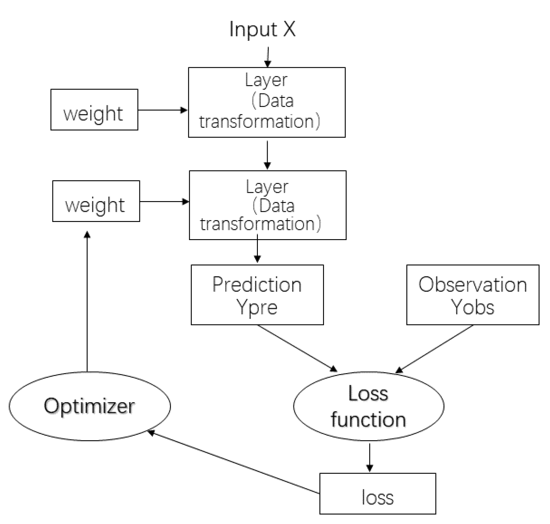
The relationship among the four factors is shown in Figure 2. Multiple layers are linked together, forming a network, and the input data are mapped into predicted values by the network. Then, the loss function compares these predicted values with targets and obtains the loss values, measuring the matching degree between predicted values and targets. Optimizer updates the weight of network by the loss value. The first order optimization algorithm is Gradient Descent.
This paper uses the neural network algorithm to investigate the relationship between the meteorological and chemical factors and the visibility from the training data set. The neural network algorithm uses meteorological and chemical factors over the Jiangsu province to automatically extract features that can be used to invert the visibility. A one-way propagation multi-layer feedforward network is used in this paper. The meteorological and chemical factors can be treated as neurons of the input layer. Moreover, each of the three hidden layers has 64 units. The input signal passes through each hidden layer in turn to the output layer node.
2.4. Error Analysis Method
In general, four error analysis methods are available, including correlation coefficient (R), root mean square error (RMSE), mean fractional error (MFE), and mean fractional bias (MFB) [42]. In numerical simulation, a model performance goal is met when both MFE and MFB are less than or equal to +50% and ±30%, respectively. This standard is also used in the verification of model products in our study.
In the above equations, S and O represent the simulated and observed sequence, respectively. The number of samples is n, and sample i is recorded as S (i) and O (i), respectively. Cov (S, O) is the covariance of S and O. Var (S) and Var (O) are the variances of S and O, respectively.
2.5. Observation Data
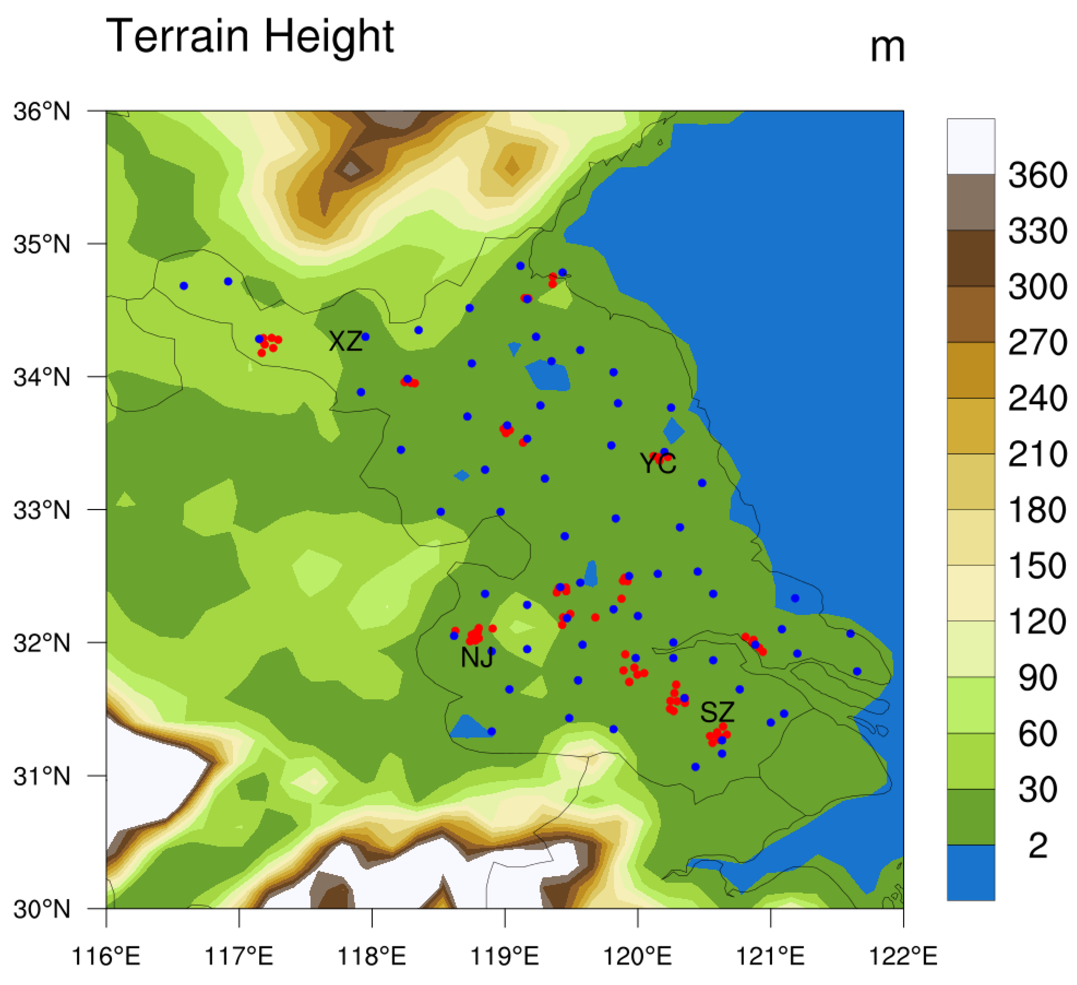
The environmental monitoring data are hourly monitoring data of atmospheric chemical composition obtained from 72 environmental monitoring stations in Jiangsu Province from 2013 to 2017. The chemical components include SO2, NO2, PM10, PM2.5, CO, and O3. The location distribution of the 72 stations is marked by red dots in Figure 3. As noted in Figure 2, rather than being evenly distributed throughout the area of Jiangsu Province, these monitoring stations are centered on cities. Therefore, when analyzing a city, the results of all the monitoring station in this city are equally weighted and averaged as the monitoring values of atmospheric chemical composition of the city.
Meteorological observation data adopt the 3-hourly surface observation data from 70 stations, including 3 national base stations, 21 basic stations, and 46 general stations in Jiangsu Province. The data contain surface air temperature measured at 2 m above ground, relative humidity, wind direction, weather phenomena, visibility, precipitation, and other meteorological elements. As noted in Figure 2, the locations of 70 stations marked by blue dots are distributed evenly in Jiangsu Province.
3. Simulation Result Analysis
3.1. Simulation of Meteorological Elements in Jiangsu Province
The model results are interpolated to the locations of 70 meteorological stations in Jiangsu Province. Further, the simulated regional average value is compared with the observed average value of 70 stations to test the ability of the WRF-Chem model to simulate the winter meteorological elements in Jiangsu Province from 2013 to 2017.
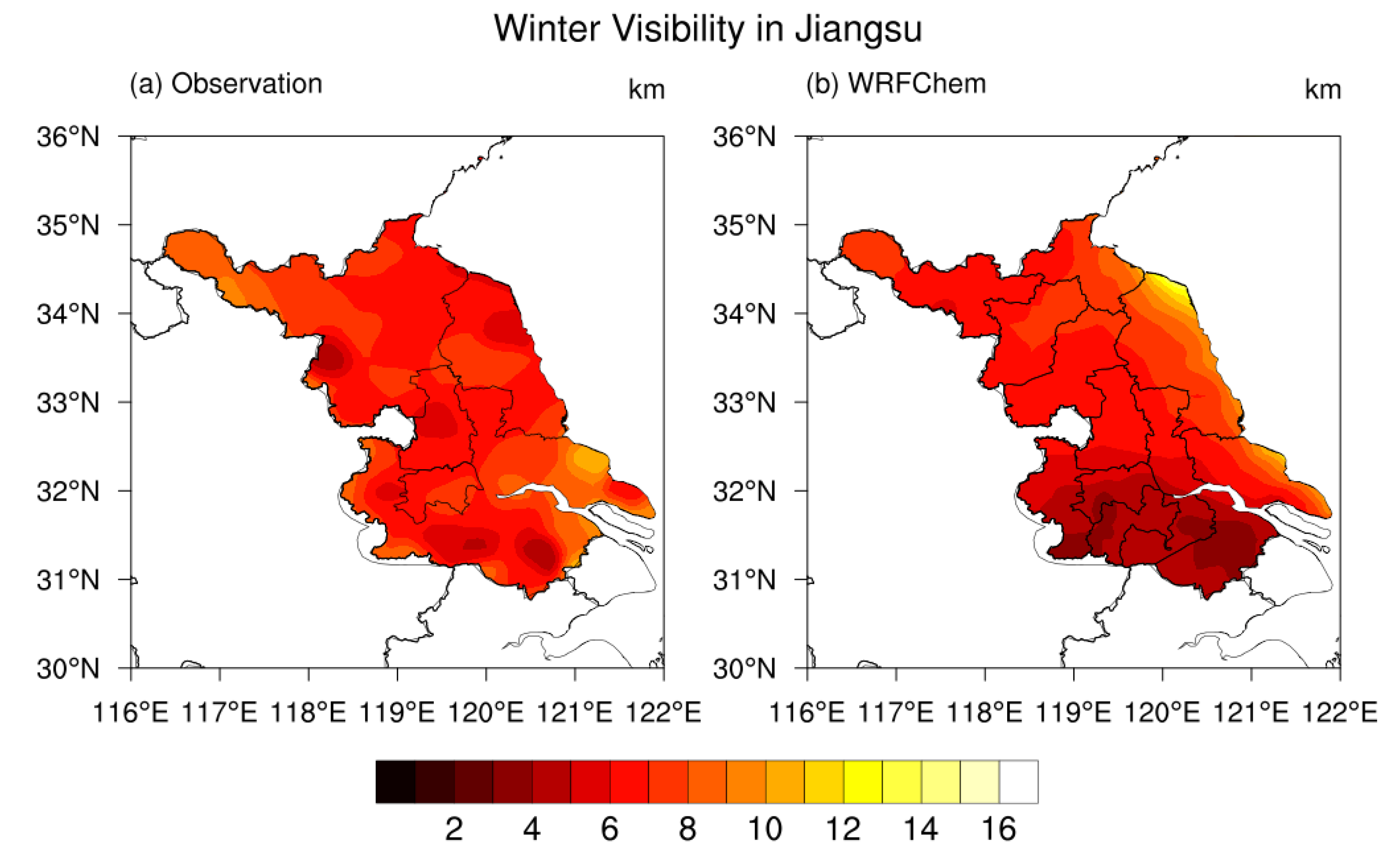
The observed and simulated spatial distribution of 2013–2017 winter mean visibility in Jiangsu province is shown in Figure 4. The winter mean visibility is lower than 8 km over most of the area, which can be well reproduced by WRF-Chem. However, the simulation somewhat overestimates and underestimates the visibility in the northern and southern part, respectively, which means the haze events could be underestimated and overestimated correspondingly.
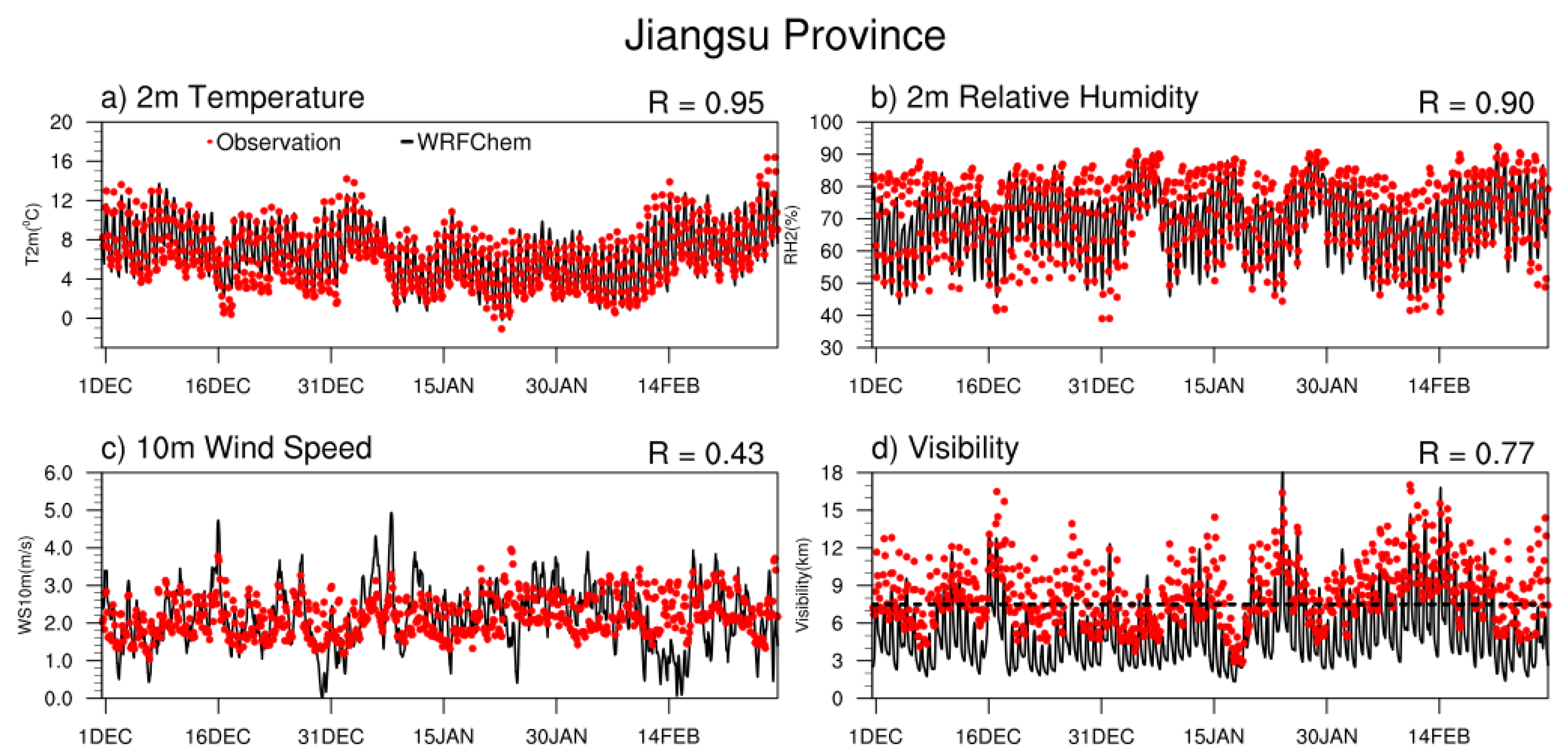
Figure 5 shows the observed and simulated data by the WRF-Chem model in winters of 2013–2017 in Jiangsu Province. The data include the 2-m air temperature (T2), 2-m relative humidity (RH2), 10-m wind speed (WS10) and the time series of visibility (VIS). The 3-hourly observation data are rendered in scattered red dots. The WRF-Chem model outputs once an hour as marked by a black curve. The value at the upper right corner is the correlation coefficient (R) of the observed and simulated 3-hourly data. As the observation’s time step is 3-hour, the length of the time series used for statistical calculation is 720. To evaluate the simulation quantitatively, the statistics of meteorological variables obtained from observation and simulation are also calculated, as shown in Table 1. As presented in Figure 5 and Table 1, the most effective simulation is the temporal variation of T2 with an R reaching 0.95, followed by the simulation of the temporal variation of RH2 with an R of approximately 0.9. In addition, the mean relative error of visibility in Table 1 is minus 32% and is close to the standard of 30%. Additionally, the mean relative deviation is less than 50%. Hence, the inversion results are generally useful. Moreover, the inverted visibility obtained from output products from WRF-Chem model is also highly correlated with the actual observation with an R of 0.77. The black dotted line in Figure 5d represents the visibility threshold of haze events (7.5 km), and the number of haze days inverted by WRF-Chem overestimates the observed data obviously.
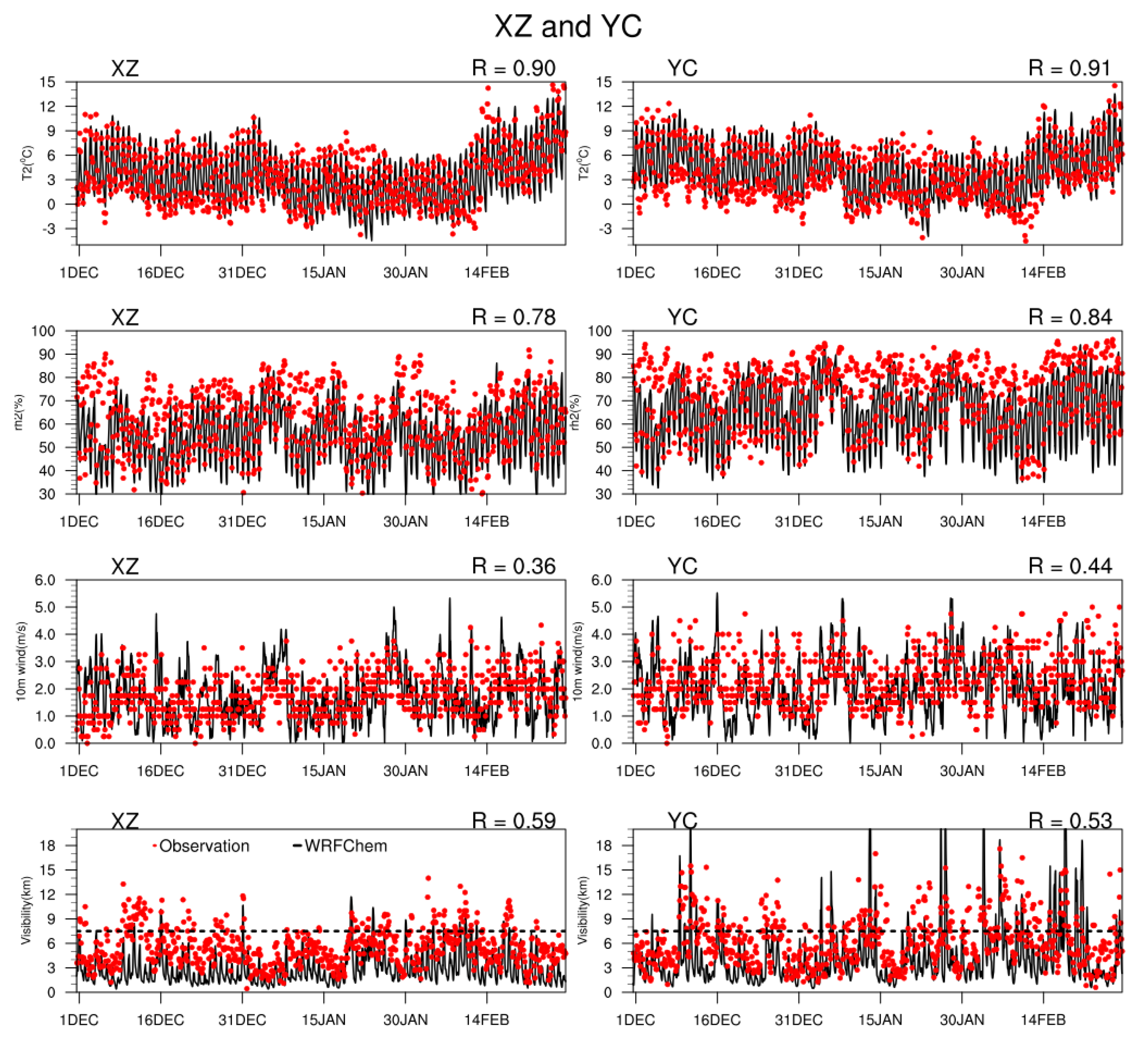
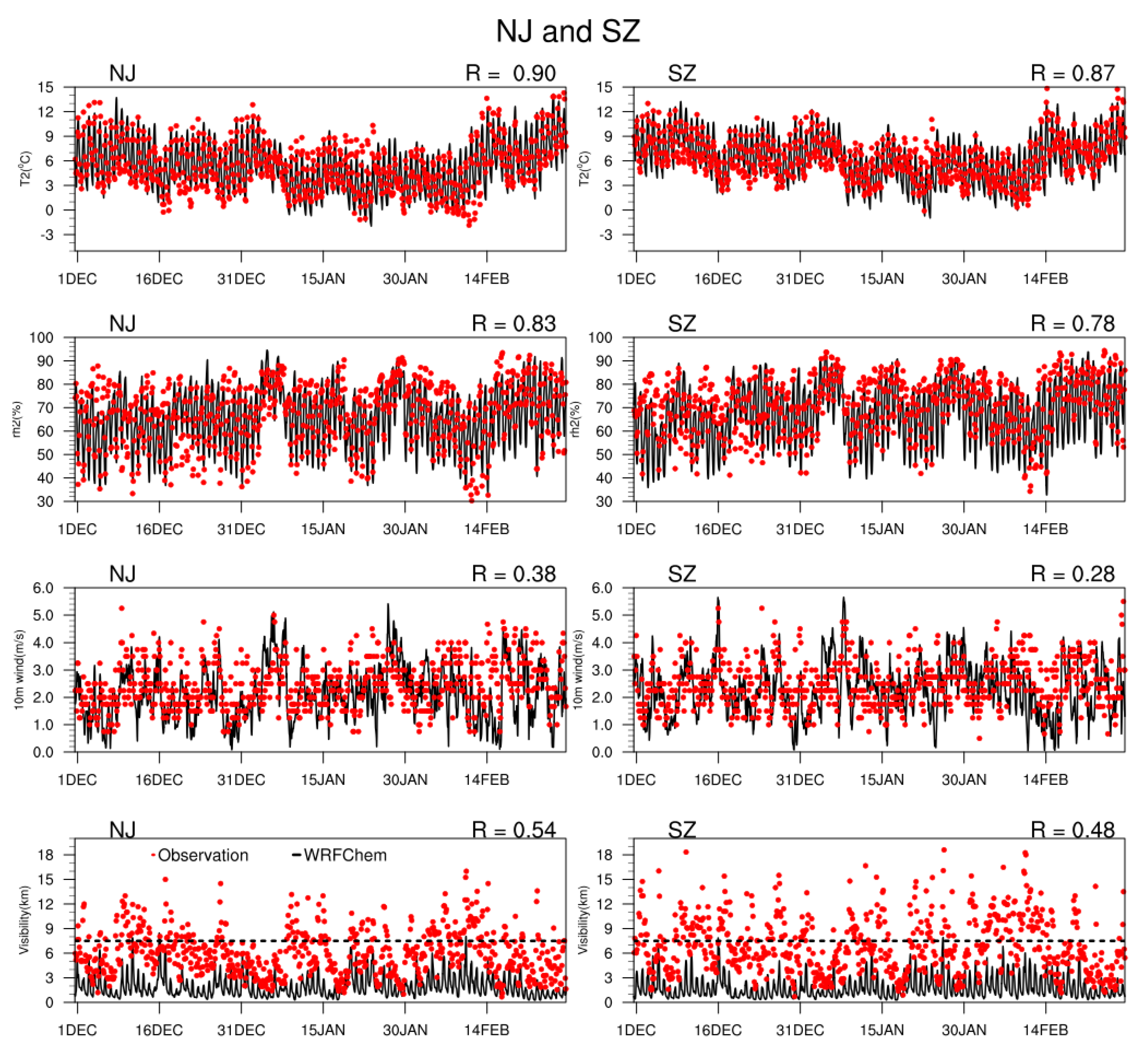
To test in detail the ability of the WRF-Chem model to simulate urban meteorological elements and the inverted visibility, four representative cities in Jiangsu Province were selected, namely, Xuzhou City (XZ), Yancheng City (YC), Nanjing City (NJ), and Suzhou City (SZ). The locations of these four cities, which are shown in Figure 3, are as follows: Xuzhou City is located in the extreme northwest of Jiangsu Province close to Shandong Province; Yancheng City is located on the east coast of Jiangsu Province and has the longest coastline in Jiangsu Province; Nanjing is located in the southwest of Jiangsu Province, bordering Anhui Province; and Suzhou is located in the south of Jiangsu Province near Shanghai. Figure 6 and Figure 7 show the mean values of T2, RH2, and WS10 obtained from observation and WRF-Chem model inversion in the winters of 2013–2017 in these four cities as well as the time series of VIS from observation and inversion based on WRF-Chem products. Meanwhile, the statistics of each meteorological variable obtained from observations and simulations are also calculated, as shown in Table 2. Similar to the simulation results in Jiangsu Province, the simulation of temporal variation of T2 in each city is the most effective, with an R of approximately 0.90, followed by the temporal variation of RH2, with an R of approximately 0.8. Moreover, the average relative errors of all variables in Table 2 are within the range of minus 30% and plus 30%, and the average relative deviation is less than 50%, which meet the standards of accurate simulation. The inverted visibility obtained from output products based on the WRF-Chem model is also highly correlated with the actual data, with an R of approximately 0.5. The dotted line in the visibility curve figure is the visibility threshold of haze (7.5 km). The visibility curve and scattering points of XZ for most of the wintertime are below the dotted line. This could be attributed to that XZ is located in the northwest of Jiangsu Province with a prevalent northwest wind in winter. Thus, air pollutants are continuously transported from North China and Central China, resulting in frequent low-visibility weather in XZ in winter. The visibility of YC is obviously higher than that of XZ. The visibility of YC inverted by WRF-Chem can reach a maximum of 77 km. This is mainly because YC is located on the eastern coast of Jiangsu Province, and the strong local sea–land wind helps to remove pollutants. On the whole, the ground meteorological elements simulated by WRF-Chem and the values and temporal variation of visibility obtained from inversion are in good agreement with the observations.
3.2. WRF-Chem Simulation of Air Pollutants in Jiangsu Province
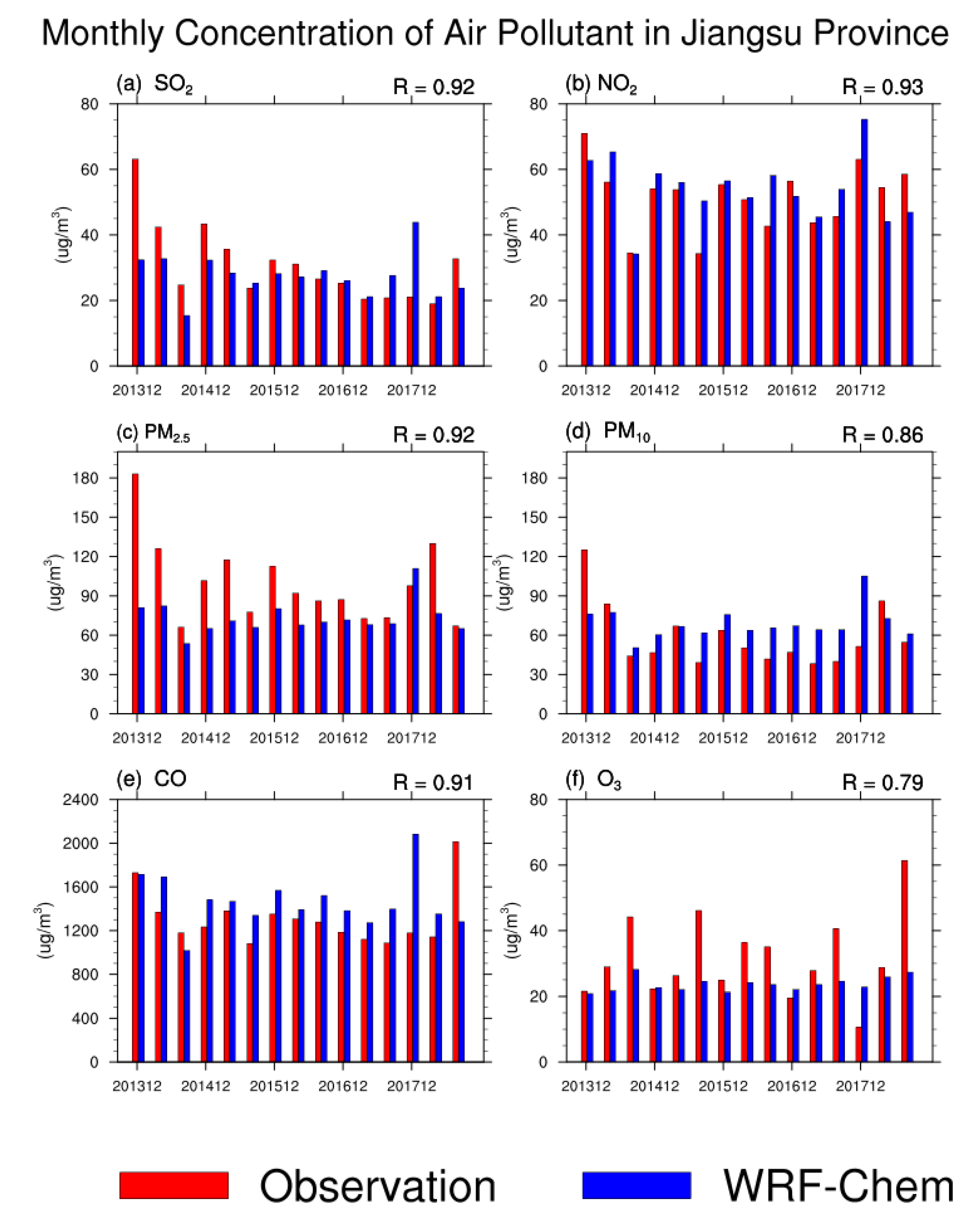
The monthly mean concentrations of SO2, NO2, PM2.5, PM10, CO, and O3 in Jiangsu Province during the winters of 2013–2017 obtained from the observation and WRF-Chem simulation are shown in Figure 8. WRF-Chem has a good ability to simulate the monthly variation of pollutants in Jiangsu Province in winter. Nevertheless, exceptions of underestimating PM2.5 and overestimating PM10 are also observed.
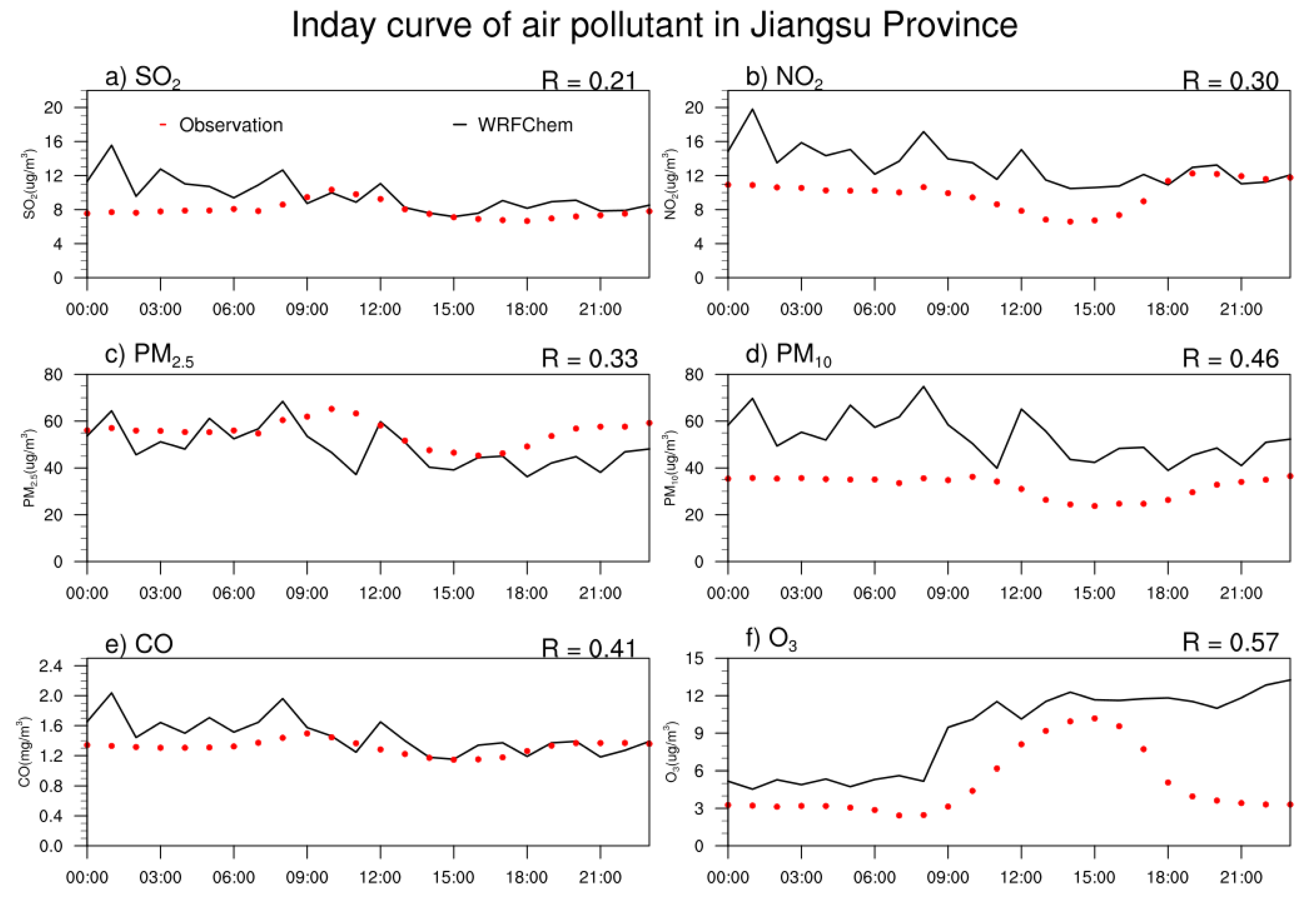
Figure 9 shows the diurnal variation curves of SO2, NO2, PM2.5, PM10, CO, and O3 obtained from observation and WRF-Chem simulation. SO2, NO2, PM2.5, PM10, and CO have similar diurnal variations. The concentration begins to increase at approximately 08:00 LST and then slowly declines in the afternoon, reaching the lowest level at approximately 15:00 LST. Then, the value increases again and becomes steady after approximately 17:00 LST. The variation is mainly due to human activities. In the rush hours of approximately 08:00 LST and 17:00 LST, automobile emissions are significantly higher, thus resulting in an increase in pollutants. The variation curve of O3 also begins to increase at approximately 08:00 LST followed by a peak observed at 15:00 LST. Then, levels begin to decline and are relatively stable after 19:00 LST. This is because solar radiation is the main factor affecting the concentration of O3. The test results indicate that the R values of PM2.5, PM10, CO, and O3 obtained by WRF-Chem simulation pass the 90% confidence test (R threshold is 0.33). The simulation reasonably reproduces the daily variation characteristics of each pollutant concentration.
3.3. Test for Modified Visibility Based on the Neural Network Scheme
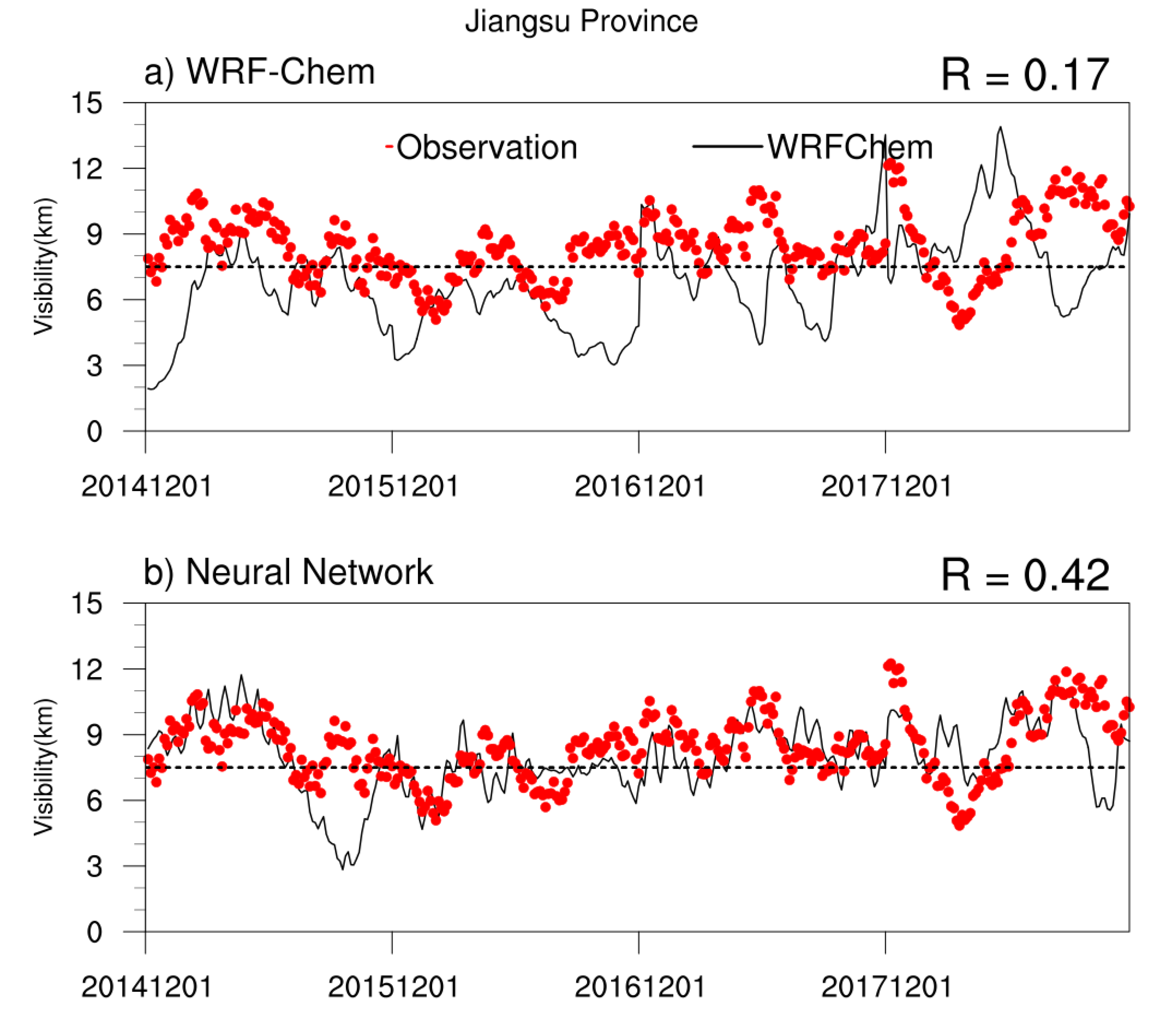
WRF-Chem shows a low ability to represent the daily visibility over Jiangsu Province. The R of the daily mean visibility between observation and inversion in winters of 2014–2017 is only 0.17 (Figure 10). Therefore, we used the neural network to modify the daily visibility series obtained from WRF-Chem inversion.
Based on previous work on the physical linkage between weather conditions and winter haze, the contribution of near-surface temperature, wind, and other meteorological factors to the variance of haze episodes can exceed 50% [1,30,31]. Moreover, Section 3.1 also proves that WRF-Chem has a strong ability to simulate these three meteorological elements. Therefore, three variables, including 2-m temperature, 10-m meridional and zonal wind speed, obtained from WRF-Chem simulation are employed for the neural network scheme. The training period is 90 days in the winter of 2013. The daily visibility series in winters of 2014–2017 are modified, as shown in Figure 10b.
Figure 10a shows the daily visibility series in the winters of 2014–2017 obtained from observation and WRF-Chem based on extinction coefficient inversion. Notably, the visibility inverted by this method is generally underestimated. This problem also occurs in the hourly series in Figure 4. After the modification of the neural network model by introducing meteorological factors, the underestimation of the inverted visibility is mostly solved. The statistical results of R, RMSE, MFE and MFB are shown in Table 3. Remarkably, the neural network significantly improves the visibility directly inverted by WRF-Chem based on the extinction coefficient. Here, R increased from 0.17 to 0.42, and RMSE/MFE/MFB decreased from 2.62/−0.26/0.33 to 1.76/−0.05/0.12.
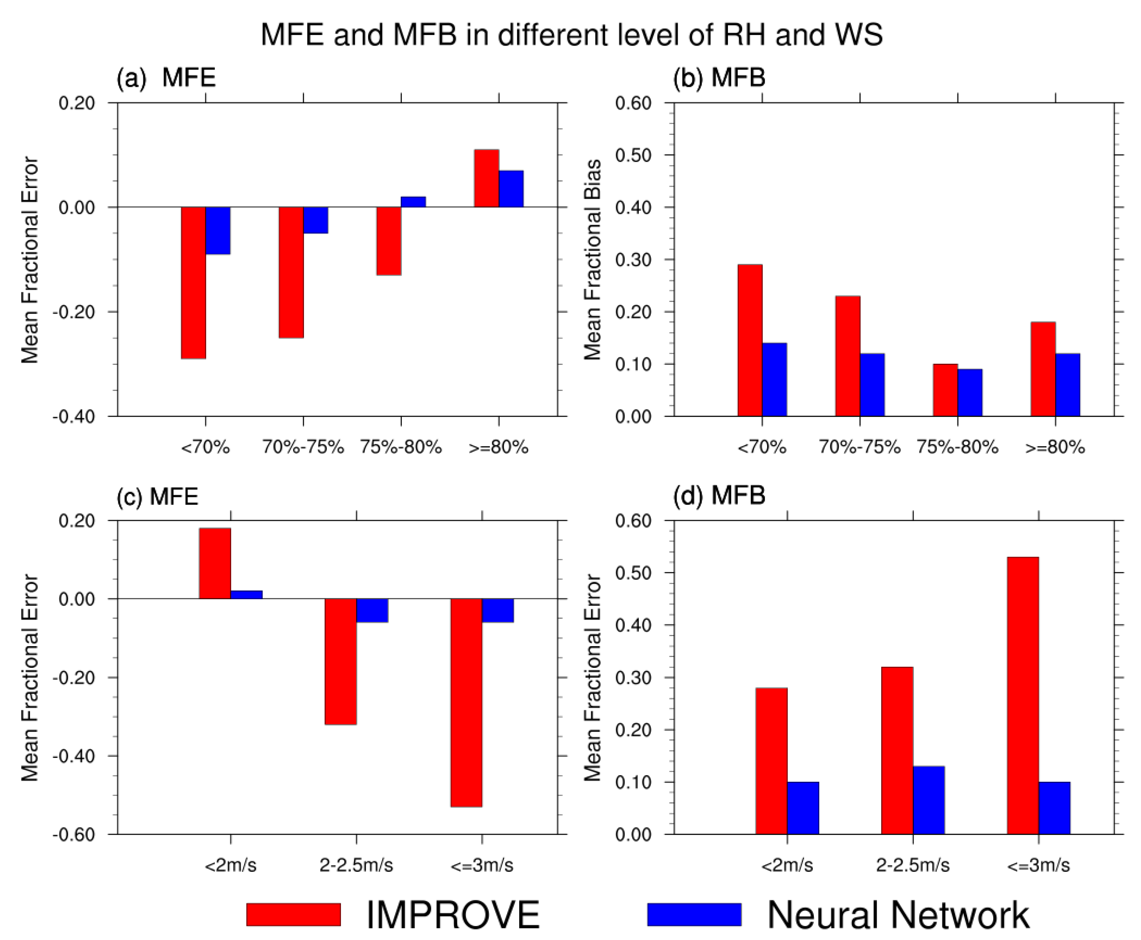
To further evaluate the correction ability of the neural network for visibility simulation, the visibility obtained from inversion is evaluated at different humidity and wind speed levels. In view of the daily series of surface relative humidity (RH) in winters of 2014–2017, there are only two days with RH less than 60% and zero days more than 90%. Therefore, the observed RH is divided into four grades, namely, RH < 70%, 70% ≤ RH < 75%, 75% ≤ RH < 80% and RH ≥ 80%. Then, the MFE and MFB of atmospheric visibility simulated by the two schemes in each grade are calculated. Similarly, wind speed (WS) is divided into three grades, namely WS < 2 m/s, 2 m/s ≤ WS < 2.5 m/s, and WS > 2.5 m/s, and the corresponding MFE and MFB are also computed. As noted in Figure 11, the visibility inversion performance of the IMPROVE extinction coefficient formula is unsatisfactory under low RH, and the visibility is significantly underestimated. However, its performance improves as RH increases. The performance of the visibility inversion scheme by the neural network is better than the IMPROVE method at each humidity level. In particular, the IMPROVE method is significantly improved under high wind speeds. For different level wind speeds, the greater the WS is, the worse the performance of the IMPROVE method. Moreover, the visibility is significantly underestimated under high WS. The performance of visibility inversion by the neural network under high WS is much better than the IMPROVE method.
4. Conclusions and Discussions
In this paper, high-resolution downscaling simulation of meteorological elements and air quality in Jiangsu Province in winters of 2013–2017 was performed using the air quality model WRF-Chem. The simulation was conducted at a spatial resolution of 18 km and a temporal resolution of 1 h. The inverted daily visibility of Jiangsu Province in winter was also calculated. The results show that WRF-Chem can accurately simulate the meteorological elements and air quality in Jiangsu Province and the four representative cities of XZ, YC, NJ, and SZ. Regarding air pollutants, NO2, PM10, and O3 are overestimated, while PM2.5 is underestimated. To some extent, the overestimation of the air pollutants leads to the low daily visibility in winter generated from the visibility inversion scheme based on the IMPROVE extinction coefficient calculation formula.
The IMPROVE extinction coefficient calculation formula mainly takes the factors of atmospheric chemical composition into account, while no meteorological factors are considered except RH. However, studies show that near-surface temperature, wind field, and other meteorological factors can contribute to greater than 50% to the variance of haze episodes. Therefore, meteorological factors that have obvious influence on visibility were employed, including 2-m air temperature, 10-m meridional and zonal wind, to improve the visibility inversion scheme based on the extinction coefficient. Considering the complex and nonlinear relationship between meteorological factors and visibility, a deep learning method, namely a neural network, was adopted. By self-modifying and modeling through machine learning, the neural network can create a modified model suitable for the simulation. The results indicate that the neural network can significantly improve the visibility inversion based on the extinction coefficient formula to solve the issue of visibility underestimation. In addition, under different RH and WS levels, the neural network has significant improvements for the IMPROVE scheme. The performance of the IMPROVE scheme to invert visibility is relatively poor under low RH or high WS, which are conducive to pollutant diffusion. Thus, the visibility is significantly underestimated. The problem is mainly caused by only considering the extinction impact of aerosol factors but leaving out meteorological factors. In short, the inverted visibility under low RH and high WS is significantly improved after introducing meteorological factors by multilayer neural network modeling.
This study fully examined the ability of the WRF-Chem model in simulating winter visibility and related meteorological variables in Jiangsu Province in eastern China. WRF-Chem reliably reproduces winter haze-related variables, especially after applying the multilayer neural network scheme. Based on this work, a dynamic downscaling study to predict the winter visibility in Jiangsu Province using WRF-Chem and the neural network scheme is on-going. Considering the possible effect of the emission and model resolution, further refinement in the emission and model resolution could help improve the simulation and prediction of regional visibility.
Author Contributions
Conceptualization, H.W., Y.Z. and P.Z.; methodology, H.W., Y.Z. and P.Z.; software, P.Z.; validation, Y.Z., P.Z. and D.L.; formal analysis, P.Z. and Y.Z.; investigation, P.Z.; resources, P.Z. and D.L.; data curation, P.Z. and D.L.; writing—original draft preparation, P.Z.; writing—review and editing, H.W. and Y.Z.; visualization, P.Z.; supervision, H.W.; project administration, Y.Z. and P.Z.; funding acquisition, Y.Z. and P.Z. All authors have read and agreed to the published version of the manuscript.
Funding
This research was funded by the National Key R&D Program of China (2017YFC1502304), and National Natural Science Foundation of China (41805001, and 41675083).
Conflicts of Interest
The authors declare no conflict of interest.
References
- Guo, Y.; Li, S.; Zhou, Y.; Chen, L.; Chen, S.; Yao, T.; Wu, S. The effect of air pollution on human physiological function in China: A longitudinal study. Lancet 2015, S31, 386. [Google Scholar] [CrossRef]
- Zanobetti, A.; Schwartz, J. The Effect of Fine and Coarse Particulate Air Pollution on Mortality: A National Analysis. Environ. Health Perspect. 2009, 117, 898–903. [Google Scholar] [CrossRef] [PubMed] [Green Version]
- Zhang, A.; Zhong, L.; Xu, Y.; Wang, H.; Dang, L. Tourists’ Perception of Haze Pollution and the Potential Impacts on Travel: Reshaping the Features of Tourism Seasonality in Beijing, China. Sustainability 2015, 7, 2397–2414. [Google Scholar] [CrossRef] [Green Version]
- Stevens, C.J.; Dise, N.B.; Mountford, J.O.; Gowing, D.J. Impact of nitrogen deposition on the species richness of grasslands. Science 2004, 303, 1876–1879. [Google Scholar] [CrossRef] [PubMed] [Green Version]
- Zhang, R.H.; Li, Q.; Zhang, R.N. Meteorological conditions for the persistent severe fog and haze event over eastern China in January 2013. Sci. China Earth Sci. 2014, 57, 26–35. [Google Scholar]
- Chen, H.P.; Wang, H.J. Haze days in North China and the associated atmospheric circulations based on daily visibility data from 1960 to 2012. J. Geophys. Res. Atmos. 2015, 120, 5895–5909. [Google Scholar] [CrossRef]
- Wang, H.J.; Chen, H.P.; Liu, J.P. Arctic sea ice decline intensified haze pollution in eastern China. Atmos. Oceanic Sci. Lett. 2015, 8, 1–9. [Google Scholar]
- Li, S.L.; Han, Z.; Chen, H.P. A comparison of the effects of interannual Arctic sea ice loss and ENSO on winter haze days: Observational analyses and AGCM simulations. J. Meteorol. Res. 2017, 31, 820–833. [Google Scholar] [CrossRef]
- Liu, D.; Wei, J.; Kang, Z.; Yan, W.; Cao, L.; Chen, H. Urbanization and Industrialization Effects on Haze in China: Take Jinagsu for Example. In Proceedings of the 19th EGU General Assembly, EGU2017, Vienna, Austria, 23–28 April 2017; 2017; p. 18493. [Google Scholar]
- Gao, X.; Xu, Y.; Zhao, Z. Jeremy Impacts of horizontal resolution and topography on the numerical simulation of East Asian precipitation (in Chinese). Chin. J. Atmos. Sci. 2006, 30, 185–192. [Google Scholar]
- Yu, E.T.; Sun, J.Q.; Chen, H.P.; Xiang, W. Evaluation of a high-resolution historical simulation over China: Climatology and extremes. Clim. Dyn. 2015, 45, 2013–2031. [Google Scholar] [CrossRef]
- Wang, J.; Wang, H.J.; Hong, Y. Comparison of satellite-estimated and model-forecasted rainfall data during a deadly debris-flow event in Zhouqu, Northwest China. Atmos. Ocean. Sci. Lett. 2016, 9, 139–145. [Google Scholar] [CrossRef] [Green Version]
- Wei, W.; Lv, Z.F.; Li, Y.; Wang, L.; Cheng, S. A WRF-Chem model study of the impact of VOCs emission of a huge petro-chemical industrial zone on the summertime ozone in Beijing, China. Atmos. Environ. 2017, 175, 44–53. [Google Scholar] [CrossRef]
- Zhou, G.; Xu, J.; Xie, Y.; Chang, L.; Gao, W.; Gu, Y. Numerical air quality forecasting over eastern China: An operational application of WRF-Chem. Atmos. Environ. 2017, 153, 94–108. [Google Scholar] [CrossRef]
- Song, H.; Wang, K.; Zhang, Y.; Hong, C.; Zhou, S. Simulation and evaluation of dust emissions with WRF-Chem (v3.7.1) and its relationship to the changing climate over East Asia from 1980 to 2015. Atmos. Environ. 2017, 167, 511–522. [Google Scholar] [CrossRef]
- Peng, H.; Liu, D.; Zhou, B.; Su, Y.; Wu, J.; Shen, H. Boundary-Layer Characteristics of Persistent Regional Haze Events and Heavy Haze Days in Eastern China. Adv. Meteorol. 2016, 2016, 1–23. [Google Scholar]
- Dai, Z.; Liu, D.; Yu, K.; Cao, L.; Jiang, Y. Meteorological Variables and Synoptic Patterns Associated with Air Pollutions in Eastern China during 2013–2018. Int. J. Environ. Res. Public Health 2020, 17, 2528. [Google Scholar] [CrossRef] [Green Version]
- Li, Z.H.; Liu, D.Y.; Yan, W.L.; Wang, H.B.; Zhu, C.Y.; Zhu, Y.Y.; Zu, F. Dense fog burst reinforcement over Eastern China: A review. Atmos. Res. 2019, 230, 104639. [Google Scholar] [CrossRef]
- Liu, Y.Z.; Wang, B.; Zhu, Q.Z.; Luo, R.; Wu, C.Q.; Jia, R. Dominant synoptic patterns and their relationships with PM2.5 pollution in winter over the Beijing-Tianjin-Hebei and Yangtze River Delta Regions. J. Meteor. Res. 2019, 33, 765–776. [Google Scholar] [CrossRef]
- Relvas, H.; Miranda, A.I. An urban air quality modeling system to support decision-making: Design and implementation. Air. Qual. Atmos. Health 2018, 11, 815–824. [Google Scholar] [CrossRef]
- Claudio, C.; Giovanna, F.; Enrico, P.; Marialuisa, V. Neuro-fuzzy and neural network systems for air quality control. Atmos. Environ. 2009, 43, 4811–4821. [Google Scholar]
- Grell, G.A.; Peckham, S.E.; Schmitz, R. Fully coupled “online” chemistry within the WRF model. Atmospheric Environment. 2005, 2005, 6957–6975. [Google Scholar] [CrossRef]
- Kain, J.S. The Kain-Fritsch convective parameterization: An update. J. Appl. Meteorol. Climatol. 2004, 43, 170–181. [Google Scholar] [CrossRef] [Green Version]
- Chen, S.-H.; Sun, W.-Y. A One-dimensional Time Dependent Cloud Model. J. Meteorol. Soc. Japan. Ser. II. 2002, 80, 99–118. [Google Scholar] [CrossRef] [Green Version]
- Baek, S. A revised radiation package of G-packed McICA and two-stream approximation: Performance evaluation in a global weather forecasting model. J. Adv. Modeling Earth Syst. 2017, 9, 3. [Google Scholar] [CrossRef]
- Hong, S.Y.; Noh, Y.; Dudhia, J. A new vertical diffusion package with an explicit treatment of entrainment processes. Mon. Weather Rev. 2006, 134, 2318–2341. [Google Scholar] [CrossRef] [Green Version]
- Chen, F.; Dudhia, J. Coupling an advanced land surface hydrology model with the Penn State–NCARMM5 modeling system. Part I: Model implementation and sensitivity. Mon. Weather Rev. 2001, 129, 569–585. [Google Scholar] [CrossRef] [Green Version]
- Jose, R.S.; Perez, J.L.; Balzarini, A.; Baro, R.; Curci, G.; Forkel, R. Sensitivity of feedback effects in CBMZ/MOSAIC chemical mechanism. Atmos. Environ. 2015, 115, 646–656. [Google Scholar] [CrossRef] [Green Version]
- Fast, J.D.; Gustafson, J.; Zaveri, R.C. Evolution of ozone, particulates, and aerosol direct forcing in an urban area using a new fully-coupled meteorology, chemistry, and aerosol model. J. Geophys. Res. 2006, 2006, D21305. [Google Scholar] [CrossRef]
- Chapman, E.C.; Gustafson, W.I.; Easter, R.C. Coupling aerosol-cloud-radiative processes in the WRF-Chem model: Investgating the radiative impact of elevated point source. Atmos. Chem. Phys. 2009, 9, 945–964. [Google Scholar] [CrossRef] [Green Version]
- Zhang, Y.; Wen, X.Y.; Jang, C.J. Simulating chemistry–aerosol–cloud–radiation–climate feedbacks over the continental U.S. using the online-coupled Weather Research Forecasting Model with chemistry (WRF/Chem). Atmos. Environ. 2010, 44, 3568–3582. [Google Scholar] [CrossRef]
- Zhang, Q.; Streets, D.G.; Carmichael, G.R.; He, K.B.; Huo, H.; Kannari, A.; Klimont, Z.; Park, I.S.; Reddy, S.; Fu, J.S.; et al. Asian emissions in 2006 for the NASA INTEXB mission. Atmos. Chem. Phys. 2009, 9, 5131–5153. [Google Scholar] [CrossRef] [Green Version]
- Li, K.; Liao, H.; Mao, Y.H.; David, A.R. Source sector and region contributions to concentration and direct radiative forcing of black carbon in China. Atmos. Environ. 2015, 124, 351–366. [Google Scholar] [CrossRef]
- Li, M.; Zhang, Q.; Streets, D.G.; He, K.B.; Cheng, Y.F.; Emmons, L.K.; Huo, H.; Kang, S.C.; Lu, Z.; Shao, M.; et al. Mapping Asian anthropogenic emissions of non-methane volatile organic compounds to multiple chemical mechanisms. Atmos. Chem. Phys. 2014, 14, 5617–5638. [Google Scholar] [CrossRef] [Green Version]
- Zheng, B.; Huo, H.; Zhang, Q.; Yao, Z.L.; Wang, X.T.; Yang, X.F.; Liu, X.; He, K.B. High-resolution mapping of vehicle emissions in China in 2008. Atmos. Chem. Phys. 2014, 14, 9787–9805. [Google Scholar] [CrossRef] [Green Version]
- Sisler, J.F.; Malm, W.C. Interpretation of trends of PM2.5 and reconstructed visibility from the IMPROVE network. J. Air Waste Manag. Assoc. 2000, 50, 775–789. [Google Scholar] [CrossRef] [PubMed]
- Chow, J.C.; Bachmann, J.D.; Wierman, S.S.G.; Chow, J.C.; Bachmann, J.D.; Wierman, S.S.G.; Mathai, C.V.; Malm, W.C.; &White, W.H. Vsibility: Science and regulation. J. Air Waste Manag. Assoc. 2002, 52, 973–999. [Google Scholar] [CrossRef] [PubMed] [Green Version]
- Pitchford, M.; Main, W.; Schichtel, B. Revised algorithm for estimating light extinction from IMPROVE particle speciation data. J. Air Waste Manag. Assoc. 2007, 57, 1326–1336. [Google Scholar] [CrossRef]
- Qiu, Y.; Ma, Z.; Li, K. A modeling study of the peroxyacetyl nitrate (PAN) during a wintertime haze event in Beijing, China. Sci. Total Environ. 2019, 650, 1944–1953. [Google Scholar] [CrossRef]
- Zhang, Z.; Gong, D.; Mao, R.; Kim S., J.; Xu, J.; Zhao, X. Cause and predictability for the severe haze pollution in downtown Beijing in November–December 2015. Sci. Total Environ. 2017, 592, 627–638. [Google Scholar] [CrossRef]
- Chollet, F. Deep Learning with Python; Manning Publications: Westampton, NJ, USA, 2018. [Google Scholar]
- Boylan, J.W.; Russell, A.G. PM and light extinction model performance metrics, goals, and criteria for three-dimensional air quality models. Atmos. Environ. 2006, 40, 4946–4959. [Google Scholar] [CrossRef]
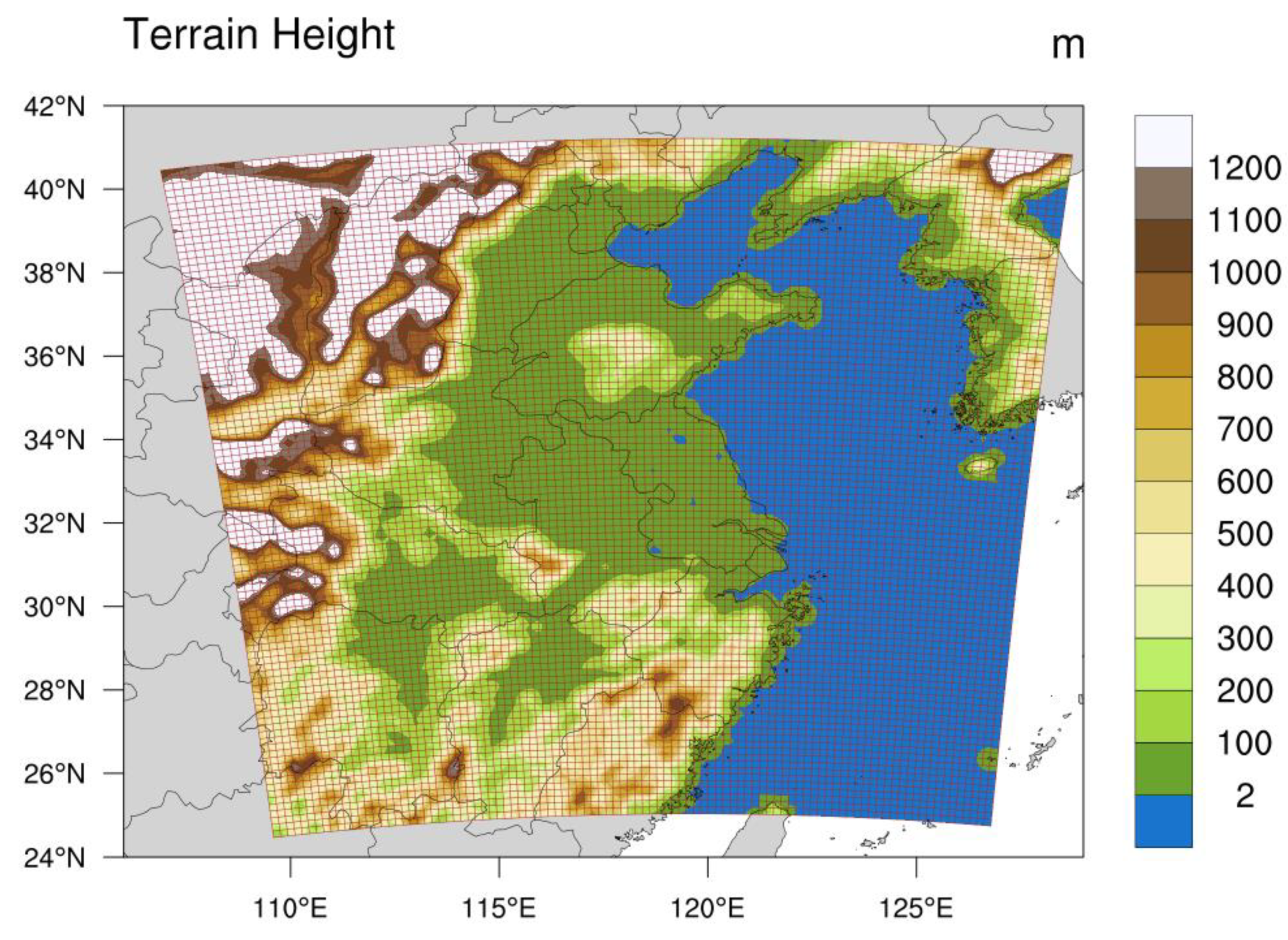
Figure 1.
Simulation domain in WRF-Chem (the grid interval is 18 km).

Figure 2.
Relationship among network, layer, loss function, and optimizer.

Figure 3.
Locations of 72 environmental monitoring stations (red dot) and 70 meteorological observation stations (blue dot) in Jiangsu Province.
Figure 3.
Locations of 72 environmental monitoring stations (red dot) and 70 meteorological observation stations (blue dot) in Jiangsu Province.

Figure 4.
Mean visibility in winters of 2013–2017 in Jiangsu Province based on (a) observation and (b) WRF-Chem model output products.
Figure 4.
Mean visibility in winters of 2013–2017 in Jiangsu Province based on (a) observation and (b) WRF-Chem model output products.

Figure 5.
The temporal variation of multi-winter (2013–2017) mean 3-hourly (a) 2m temperature, (b) 2m relative humidity, (c) 10m wind speed, (d) visibility in Jiangsu province in observation (red spots) and WRF-Chem simulation (black curves).
Figure 5.
The temporal variation of multi-winter (2013–2017) mean 3-hourly (a) 2m temperature, (b) 2m relative humidity, (c) 10m wind speed, (d) visibility in Jiangsu province in observation (red spots) and WRF-Chem simulation (black curves).

Figure 6.
The temporal variation of multi-winter (2013–2017) mean 3-hourly T2, RH2, WS10, and VIS from top to bottom, obtained from observation (red dots) and WRF-Chem simulation (black curves) in the city of Xuzhou City (XZ) (left column) and Yancheng City (YC) (right column).
Figure 6.
The temporal variation of multi-winter (2013–2017) mean 3-hourly T2, RH2, WS10, and VIS from top to bottom, obtained from observation (red dots) and WRF-Chem simulation (black curves) in the city of Xuzhou City (XZ) (left column) and Yancheng City (YC) (right column).

Figure 7.
The temporal variation of multi-winter (2013–2017) mean 3-hourly T2, RH2, WS10, and VIS from top to bottom, obtained from observation (red dots) and WRF-Chem simulation (black curves) in the city of Nanjing City (NJ) (left column) and Suzhou City (SZ) (right column).
Figure 7.
The temporal variation of multi-winter (2013–2017) mean 3-hourly T2, RH2, WS10, and VIS from top to bottom, obtained from observation (red dots) and WRF-Chem simulation (black curves) in the city of Nanjing City (NJ) (left column) and Suzhou City (SZ) (right column).

Figure 8.
Comparison of monthly mean atmospheric pollutant concentrations between observation and WRF-Chem simulation in winters of 2013–2017.
Figure 8.
Comparison of monthly mean atmospheric pollutant concentrations between observation and WRF-Chem simulation in winters of 2013–2017.

Figure 9.
Diurnal variation curves of SO2, NO2, PM2.5, PM10, CO, and O3 obtained from observation and WRF-Chem modulation. The R thresholds of passing 90% and 95% confidence tests are 0.33 and 0.388, respectively.
Figure 9.
Diurnal variation curves of SO2, NO2, PM2.5, PM10, CO, and O3 obtained from observation and WRF-Chem modulation. The R thresholds of passing 90% and 95% confidence tests are 0.33 and 0.388, respectively.

Figure 10.
Time series of daily mean visibility obtained from observation and WRF-Chem model simulation corrected by the neural network in Jiangsu Province in winters of 2014–2017.
Figure 10.
Time series of daily mean visibility obtained from observation and WRF-Chem model simulation corrected by the neural network in Jiangsu Province in winters of 2014–2017.

Figure 11.
MFE and MFB derived from visibility of different surface relative humidity and wind speed levels by Interagency Monitoring of Protected Visual Environments (IMPROVE) and neural network observations.
Figure 11.
MFE and MFB derived from visibility of different surface relative humidity and wind speed levels by Interagency Monitoring of Protected Visual Environments (IMPROVE) and neural network observations.


Table 1.
Correlation coefficient (R), root mean square error (RMSE), mean fractional error (MFE), and mean fractional bias (MFB) of the multi-winter (2013–2017) mean 3-hourly T2, RH2, WS10, and VIS simulated by WRF-Chem model compared to the observation in Jiangsu Province.
Table 1.
Correlation coefficient (R), root mean square error (RMSE), mean fractional error (MFE), and mean fractional bias (MFB) of the multi-winter (2013–2017) mean 3-hourly T2, RH2, WS10, and VIS simulated by WRF-Chem model compared to the observation in Jiangsu Province.
| Weather Element | R | RMSE | MFE | MFB |
|---|---|---|---|---|
| T2(°C) | 0.95 | 0.97 | 0.04 | 0.11 |
| RH2(%) | 0.90 | 5.95 | −0.02 | 0.04 |
| WS10(m/s) | 0.43 | 0.75 | −0.02 | 0.19 |
| Visibility(km) | 0.76 | 3.70 | −0.32 | 0.33 |
Table 2.
R, RMSE, MFE and MFB of the multi-winter (2013–2017) mean 3-hourly T2, RH2, WS10, and VIS simulated by WRF-Chem model compared to the observation in the four cities of XZ, YC, NJ, and SZ.
Table 2.
R, RMSE, MFE and MFB of the multi-winter (2013–2017) mean 3-hourly T2, RH2, WS10, and VIS simulated by WRF-Chem model compared to the observation in the four cities of XZ, YC, NJ, and SZ.
| Weather Element | City | R | RMSE | MFE | MFB |
|---|---|---|---|---|---|
| T2(°C) | XZ | 0.90 | 1.51 | −0.22 | 0.45 |
| YC | 0.91 | 1.38 | 0.24 | 0.40 | |
| NJ | 0.90 | 1.36 | −0.16 | 0.14 | |
| SZ | 0.87 | 1.30 | 0.014 | 0.10 | |
| RH2(%) | XZ | 0.78 | 10.50 | −0.06 | 0.10 |
| YC | 0.84 | 11.26 | −0.08 | 0.09 | |
| NJ | 0.83 | 7.88 | −0.01 | 0.07 | |
| SZ | 0.78 | 9.25 | −0.04 | 0.07 | |
| WS10(m/s) | XZ | 0.36 | 1.01 | −0.02 | 0.34 |
| YC | 0.44 | 1.07 | −0.08 | 0.27 | |
| NJ | 0.38 | 1.07 | −0.08 | 0.25 | |
| SZ | 0.28 | 1.14 | 0.00 | 0.26 | |
| Visibility (VIS, km) | XZ | 0.59 | 3.16 | −0.03 | 0.26 |
| YC | 0.53 | 6.52 | 0.16 | 0.33 | |
| NJ | 0.54 | 3.26 | −0.24 | 0.34 | |
| SZ | 0.48 | 4.49 | −0.30 | 0.42 |
Table 3.
R, RMSE, MFE and MFB of daily mean visibility (360 days by length) between observation and WRF-Chem model simulation corrected by neural network in Jiangsu Province in winters of 2014–2017.
Table 3.
R, RMSE, MFE and MFB of daily mean visibility (360 days by length) between observation and WRF-Chem model simulation corrected by neural network in Jiangsu Province in winters of 2014–2017.
| Scheme | R | RMSE | MFE | MFB |
|---|---|---|---|---|
| IMPROVE | 0.17 | 2.62 | −0.26 | 0.33 |
| Neural Network | 0.42 | 1.76 | −0.05 | 0.12 |
© 2020 by the authors. Licensee MDPI, Basel, Switzerland. This article is an open access article distributed under the terms and conditions of the Creative Commons Attribution (CC BY) license (http://creativecommons.org/licenses/by/4.0/).
Share and Cite
MDPI and ACS Style
Zong, P.; Zhu, Y.; Wang, H.; Liu, D. WRF-Chem Simulation of Winter Visibility in Jiangsu, China, and the Application of a Neural Network Algorithm. Atmosphere 2020, 11, 520. https://0-doi-org.brum.beds.ac.uk/10.3390/atmos11050520
AMA Style
Zong P, Zhu Y, Wang H, Liu D. WRF-Chem Simulation of Winter Visibility in Jiangsu, China, and the Application of a Neural Network Algorithm. Atmosphere. 2020; 11(5):520. https://0-doi-org.brum.beds.ac.uk/10.3390/atmos11050520
Chicago/Turabian StyleZong, Peishu, Yali Zhu, Huijun Wang, and Duanyang Liu. 2020. "WRF-Chem Simulation of Winter Visibility in Jiangsu, China, and the Application of a Neural Network Algorithm" Atmosphere 11, no. 5: 520. https://0-doi-org.brum.beds.ac.uk/10.3390/atmos11050520
Note that from the first issue of 2016, this journal uses article numbers instead of page numbers. See further details here.