Long-Term Variability in Potential Evapotranspiration, Water Availability and Drought under Climate Change Scenarios in the Awash River Basin, Ethiopia


Abstract
:1. Introduction
2. Methodology
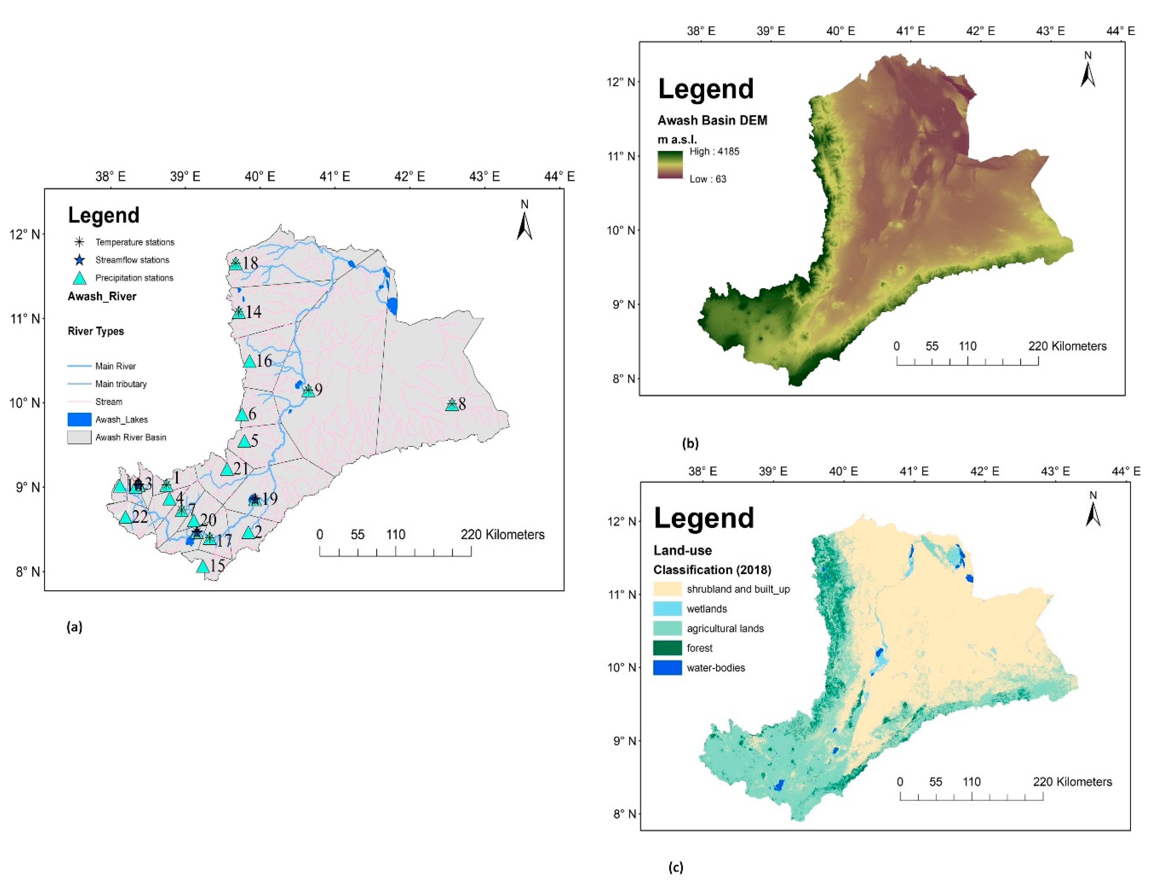
2.1. Study Area
2.2. Dataset
2.3. Data Analysis
2.3.1. Evapotranspiration
2.3.2. Water Availability
2.3.3. Drought Indices
3. Results
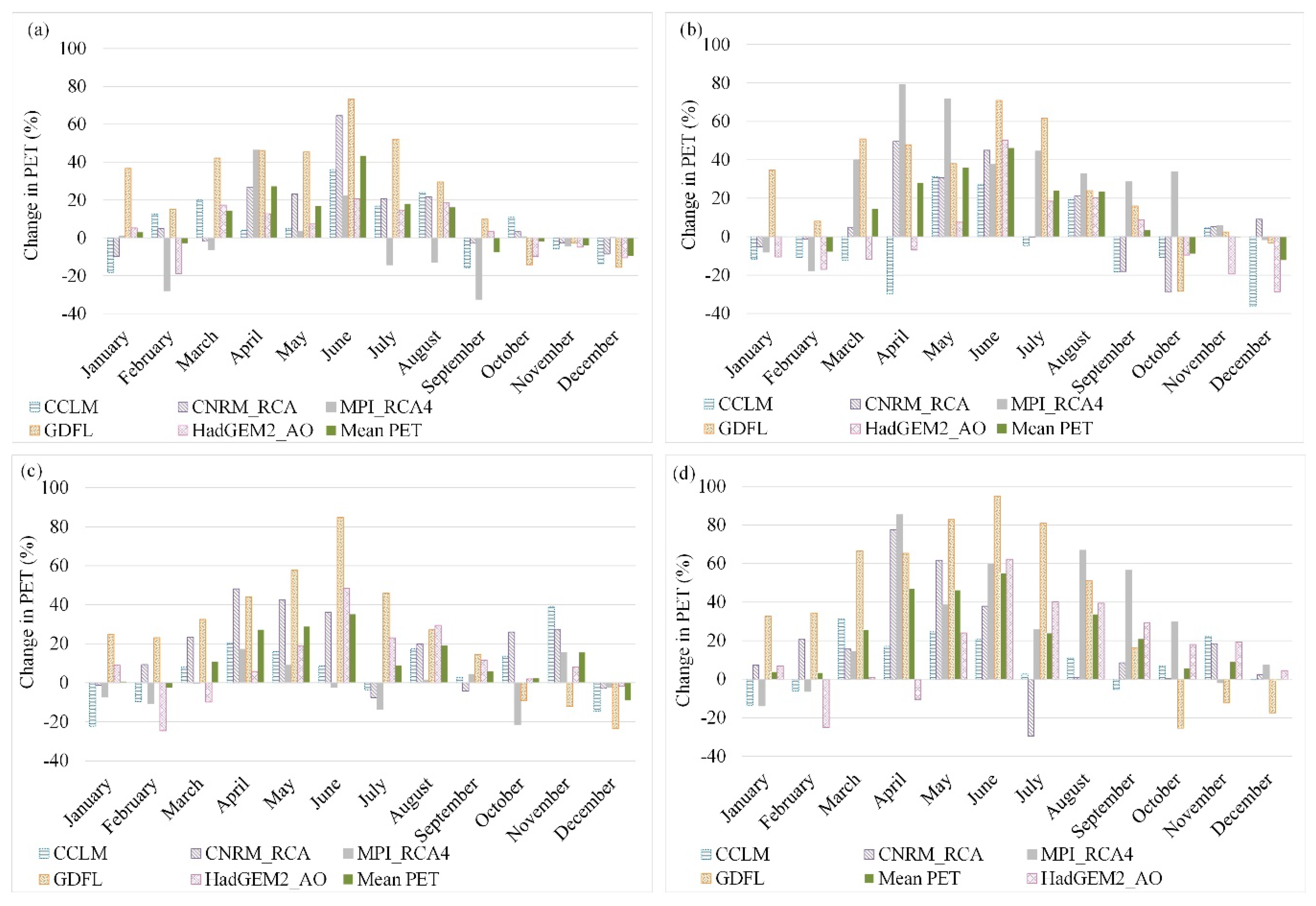
3.1. Potential Evapotranspiration (PET)
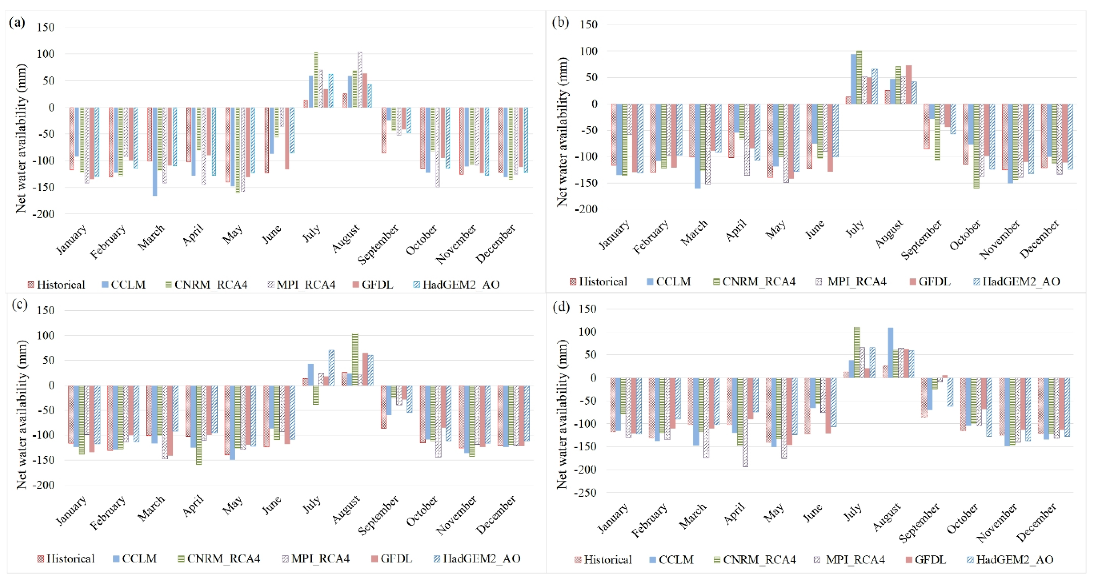
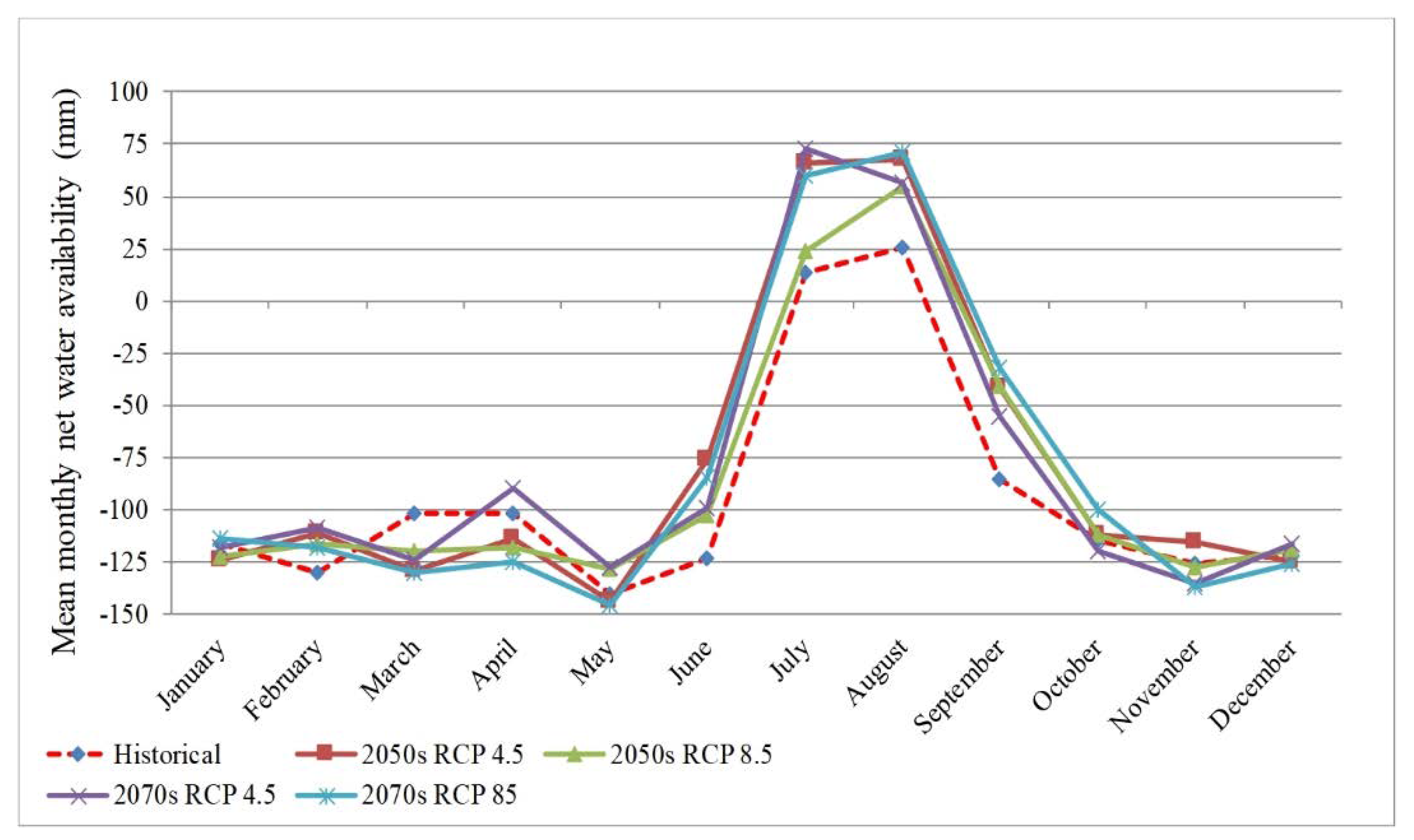
3.2. Net Water Availability
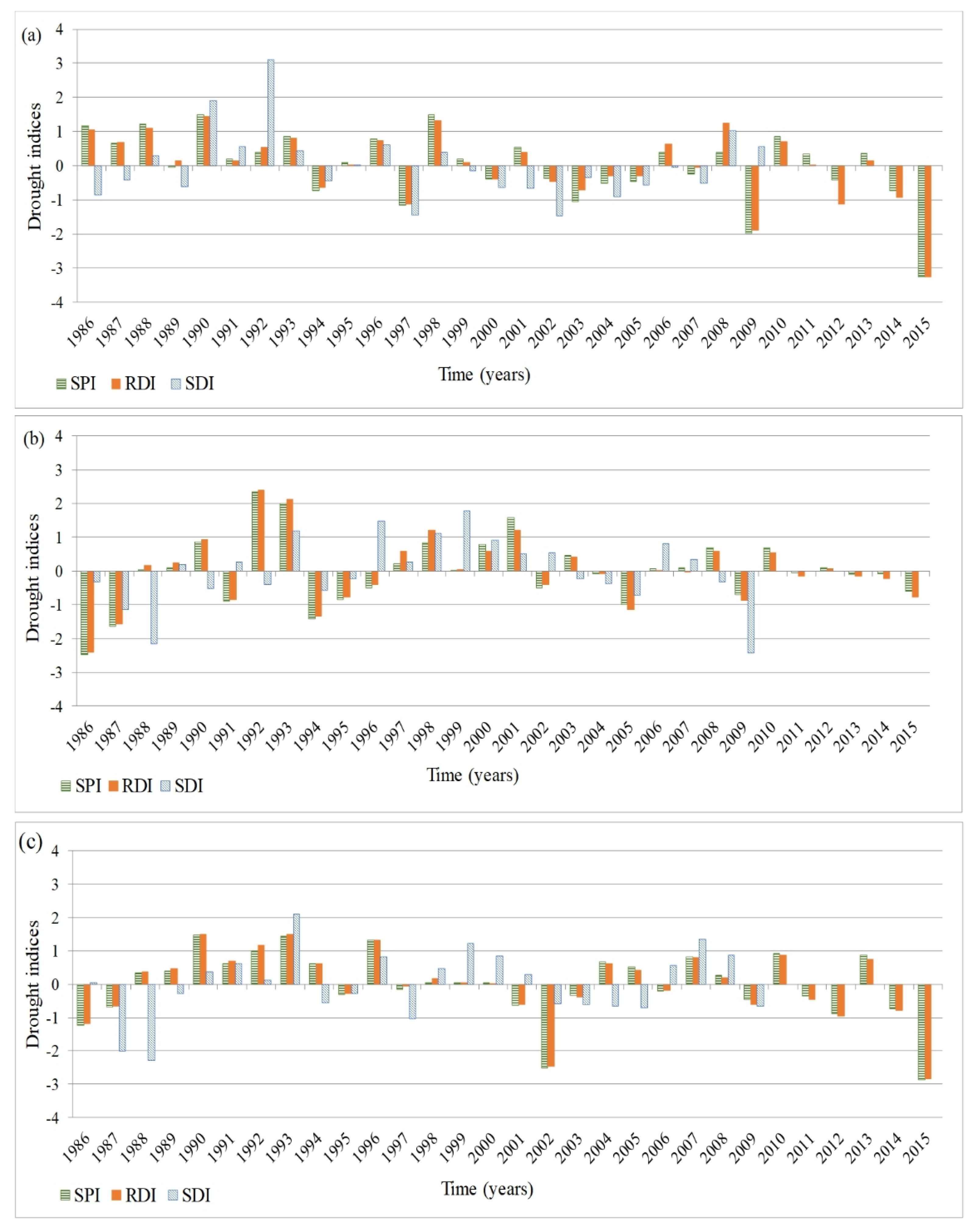
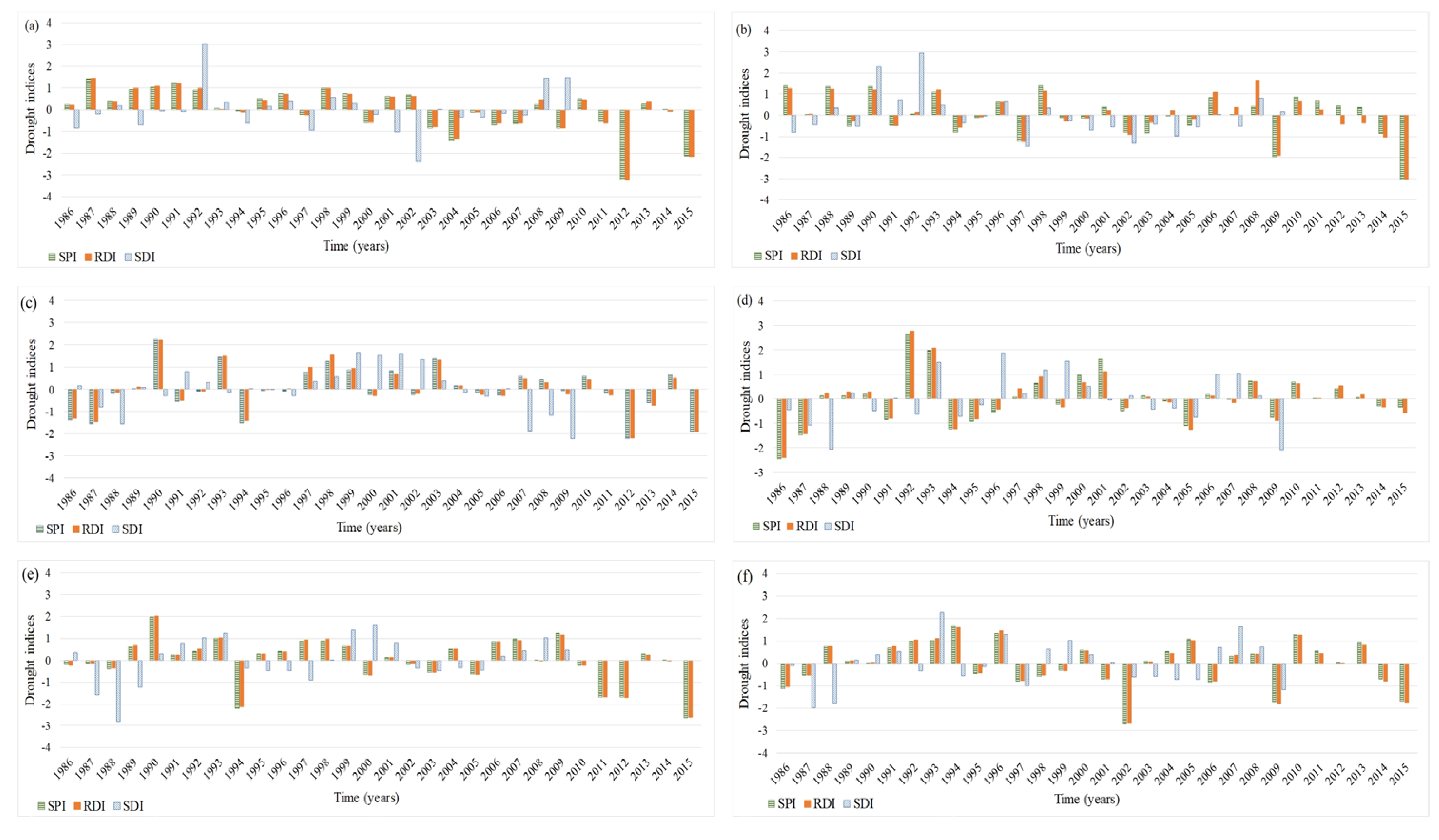
3.3. Drought Index
4. Discussion
5. Conclusions
Author Contributions
Funding
Acknowledgments
Conflicts of Interest
Appendix A

Appendix B

| 3 Months First Season | ||||||
|---|---|---|---|---|---|---|
| Locations | Index | Drought Occurrence (%) | Total | |||
| Mild | Moderate | Severe | Extreme | |||
| Holetta | SPI | 36.7 | 10.0 | 6.7 | 0.0 | 53.3 |
| RDI | 30.0 | 13.3 | 6.7 | 0.0 | 50.0 | |
| SDI | 50.0 | 0.0 | 0.0 | 4.2 | 54.2 | |
| Koka Dam | SPI | 50.0 | 0.0 | 0.0 | 0.0 | 50.0 |
| RDI | 53.3 | 0.0 | 0.0 | 0.0 | 53.3 | |
| SDI | 45.8 | 0.0 | 12.5 | 0.0 | 58.3 | |
| Metehara | SPI | 46.7 | 6.7 | 6.7 | 0.0 | 60.0 |
| RDI | 46.7 | 6.7 | 6.7 | 0.0 | 60.0 | |
| SDI | 33.3 | 12.5 | 0.0 | 4.2 | 50.0 | |
| 3 Months Second Season | ||||||
| Locations | Index | Drought Occurrence (%) | Total | |||
| Mild | Moderate | Severe | Extreme | |||
| Holetta | SPI3 | 23.3 | 6.7 | 6.7 | 3.3 | 40.0 |
| RDI3 | 23.3 | 6.7 | 6.7 | 3.3 | 40.0 | |
| SDI3 | 62.5 | 0.0 | 0.0 | 4.2 | 66.7 | |
| Koka Dam | SPI3 | 33.3 | 13.3 | 0.0 | 0.0 | 46.7 |
| RDI3 | 30.0 | 13.3 | 0.0 | 0.0 | 43.3 | |
| SDI3 | 29.2 | 16.7 | 0.0 | 4.2 | 50.0 | |
| Metehara | SPI3 | 20.0 | 3.3 | 10.0 | 0.0 | 33.3 |
| RDI3 | 20.0 | 3.3 | 10.0 | 0.0 | 33.3 | |
| SDI3 | 16.7 | 4.2 | 4.2 | 8.3 | 33.3 | |
| 3 Months Third Season | ||||||
| Locations | Index | Drought Occurrence (%) | Total | |||
| Mild | Moderate | Severe | Extreme | |||
| Holetta | SPI | 33.3 | 3.3 | 6.7 | 3.3 | 46.7 |
| RDI | 30.0 | 13.3 | 3.3 | 3.3 | 50.0 | |
| SDI | 54.2 | 0.0 | 0.0 | 4.2 | 58.3 | |
| Koka Dam | SPI | 40.0 | 6.7 | 6.7 | 0.0 | 53.3 |
| RDI | 40.0 | 6.7 | 6.7 | 0.0 | 53.3 | |
| SDI | 41.7 | 4.2 | 4.2 | 4.2 | 54.2 | |
| Metehara | SPI | 36.7 | 20.0 | 0.0 | 0.0 | 56.7 |
| RDI | 36.7 | 20.0 | 0.0 | 0.0 | 56.7 | |
| SDI | 29.2 | 4.2 | 4.2 | 4.2 | 41.7 | |
| 3 Months Fourth Season | ||||||
| Locations | Index | Drought Occurrence (%) | Total | |||
| Mild | Moderate | Severe | Extreme | |||
| Holetta | SPI | 33.3 | 10.0 | 0.0 | 3.3 | 46.7 |
| RDI | 40.0 | 6.7 | 0.0 | 3.3 | 50.0 | |
| SDI | 45.8 | 12.5 | 0.0 | 0.0 | 58.3 | |
| Koka Dam | SPI | 40.0 | 3.3 | 3.3 | 3.3 | 50.0 |
| RDI | 26.7 | 10.0 | 3.3 | 3.3 | 43.3 | |
| SDI | 54.2 | 4.2 | 4.2 | 0.0 | 62.5 | |
| Metehara | SPI | 26.7 | 13.3 | 3.3 | 3.3 | 46.7 |
| RDI | 23.3 | 13.3 | 3.3 | 3.3 | 43.3 | |
| SDI | 41.7 | 12.5 | 0.0 | 4.2 | 58.3 | |
References
- Mohammed, R.; Scholz, M. Climate Variability Impact on the Spatiotemporal Characteristics of Drought and Aridityin Arid and Semi-Arid Regions. Water Resour. Manag. 2019, 33, 5015–5033. [Google Scholar] [CrossRef] [Green Version]
- Chen, H.; Guo, S.; Xu, C.-Y.; Singh, V.P. Historical temporal trends of hydro-climatic variables and runoff response to climate variability and their relevance in water resource management in the Hanjiang basin. J. Hydrol. 2007, 344, 171–184. [Google Scholar] [CrossRef]
- Leta, O.T.; El-Kadi, A.I.; Dulai, H.; Ghazal, K.A. Assessment of climate change impacts on water balance components of Heeia watershed in Hawaii. J. Hydrol. Reg. Stud. 2016, 8, 182–197. [Google Scholar] [CrossRef] [Green Version]
- Kusangaya, S.; Warburton, M.L.; Van Garderen, E.A.; Jewitt, G.P. Impacts of climate change on water resources in southern Africa: A review. Phys. Chem. Earth Parts A/B/C 2014, 67, 47–54. [Google Scholar] [CrossRef]
- Ehlers, E.; Krafft, T. German Global Change Research; National Committee on Global Change Research: Bonn, Germany, 1998; p. 130. [Google Scholar]
- Thomas, A. Spatial and temporal characteristics of potential evapotranspiration trends over China. Int. J. Climatol. A J. R. Meteorol. Soc. 2000, 20, 381–396. [Google Scholar] [CrossRef]
- Fisher, J.B.; Melton, F.; Middleton, E.; Hain, C.; Anderson, M.; Allen, R.; McCabe, M.F.; Hook, S.; Baldocchi, D.; Townsend, P.A. The future of evapotranspiration: Global requirements for ecosystem functioning, carbon and climate feedbacks, agricultural management, and water resources. Water Resour. Res. 2017, 53, 2618–2626. [Google Scholar] [CrossRef]
- Peters, T. Water Balance in Tropical Regions; Springer: Berlin/Heidelberg, Germany, 2016; pp. 391–403. [Google Scholar] [CrossRef]
- Djaman, K.; Koudahe, K.; Ganyo, K.K. Trend analysis in annual and monthly pan evaporation and pan coefficient in the context of climate change in togo. J. Geosci. Environ. Prot. 2017, 5, 41–56. [Google Scholar] [CrossRef] [Green Version]
- Muhammad, M.K.I.; Nashwan, M.S.; Shahid, S.; Ismail, T.B.; Song, Y.H.; Chung, E.-S. Evaluation of Empirical Reference Evapotranspiration Models Using Compromise Programming: A Case Study of Peninsular Malaysia. Sustainability 2019, 11, 4267. [Google Scholar] [CrossRef] [Green Version]
- Lang, D.; Zheng, J.; Shi, J.; Liao, F.; Ma, X.; Wang, W.; Chen, X.; Zhang, M. A comparative study of potential evapotranspiration estimation by eight methods with FAO Penman–Monteith method in southwestern China. Water 2017, 9, 734. [Google Scholar] [CrossRef] [Green Version]
- Djaman, K.; Balde, A.B.; Sow, A.; Muller, B.; Irmak, S.; N’Diaye, M.K.; Manneh, B.; Moukoumbi, Y.D.; Futakuchi, K.; Saito, K. Evaluation of sixteen reference evapotranspiration methods under sahelian conditions in the Senegal River Valley. J. Hydrol. Reg. Stud. 2015, 3, 139–159. [Google Scholar] [CrossRef] [Green Version]
- Tukimat, N.N.A.; Harun, S.; Shahid, S. Comparison of different methods in estimating potential evapotranspiration at Muda Irrigation Scheme of Malaysia. J. Agric. Rural Dev. Trop. Subtrop. (JARTS) 2012, 113, 77–85. [Google Scholar]
- Lu, J.; Sun, G.; McNulty, S.G.; Amatya, D.M. A comparison of six potential evapotranspiration methods for regional use in the Southeastern United States 1. JAWRA J. Am. Water Resour. Assoc. 2005, 41, 621–633. [Google Scholar] [CrossRef]
- Douglas, E.M.; Jacobs, J.M.; Sumner, D.M.; Ray, R.L. A comparison of models for estimating potential evapotranspiration for Florida land cover types. J. Hydrol. 2009, 373, 366–376. [Google Scholar] [CrossRef]
- Pan, S.; Xu, Y.-P.; Xuan, W.; Gu, H.; Bai, Z. Appropriateness of potential evapotranspiration models for climate change impact analysis in Yarlung Zangbo River basin, China. Atmosphere 2019, 10, 453. [Google Scholar] [CrossRef] [Green Version]
- Khoshravesh, M.; Sefidkouhi, M.A.G.; Valipour, M. Estimation of reference evapotranspiration using multivariate fractional polynomial, Bayesian regression, and robust regression models in three arid environments. Appl. Water Sci. 2017, 7, 1911–1922. [Google Scholar] [CrossRef] [Green Version]
- McMahon, T.A.; Peel, M.C.; Lowe, L.; Srikanthan, R.; McVicar, T.R. Estimating actual, potential, reference crop and pan evaporation using standard meteorological data: A pragmatic synthesis. Hydrol. Earth Syst. Sci. 2013, 17, 1331–1363. [Google Scholar] [CrossRef] [Green Version]
- Hosseinzadeh Talaee, P. Performance evaluation of modified versions of Hargreaves equation across a wide range of Iranian climates. Meteorol. Atmos. Phys. 2014, 126, 65–70. [Google Scholar] [CrossRef]
- Xu, C.-Y.; Singh, V. Cross comparison of empirical equations for calculating potential evapotranspiration with data from Switzerland. Water Resour. Manag. 2002, 16, 197–219. [Google Scholar] [CrossRef]
- Berti, A.; Tardivo, G.; Chiaudani, A.; Rech, F.; Borin, M. Assessing reference evapotranspiration by the Hargreaves method in north-eastern Italy. Agric. Water Manag. 2014, 140, 20–25. [Google Scholar] [CrossRef]
- Li, Z.; Yang, Y.; Kan, G.; Hong, Y. Study on the applicability of the Hargreaves potential evapotranspiration estimation method in CREST distributed hydrological model (Version 3.0) applications. Water 2018, 10, 1882. [Google Scholar] [CrossRef] [Green Version]
- Hargreaves, G.H.; Samani, Z.A. Reference crop evapotranspiration from temperature. Appl. Eng. Agric. 1985, 1, 96–99. [Google Scholar] [CrossRef]
- Edwards, P.J.; Williard, K.W.; Schoonover, J.E. Fundamentals of watershed hydrology. J. Contemp. Water Res. Educ. 2015, 154, 3–20. [Google Scholar] [CrossRef]
- Davie, T.; Quinn, N.W. Fundamentals of Hydrology; Routledge: Oxon, UK; New York, NY, USA, 2019. [Google Scholar]
- Raghunath, H.M. Hydrology: Principles, Analysis and Design; New Age International: New Delhi, India, 2006. [Google Scholar]
- EU. Guidance Document on the Application of Water Balances for Supporting the Implementation of the WFD; European Union Technical Report; EU: Luxembourg, 2015; ISBN 978-92-79-52021-1. [Google Scholar]
- McKee, T.B.; Doesken, N.J.; Kleist, J. The relationship of drought frequency and duration to time scales. In Proceedings of the 8th Conference on Applied Climatology, Boston, MA, USA, 17–22 January 1993. [Google Scholar]
- Eslamian, S.; Ostad-Ali-Askari, K.; Singh, V.P.; Dalezios, N.R.; Ghane, M.; Yihdego, Y.; Matouq, M. A review of drought indices. Int. J. Constr. Res. Civ. Eng. (Ijrcre) 2017, 3, 48–66. [Google Scholar]
- Mishra, A.K.; Singh, V.P. A review of drought concepts. J. Hydrol. 2010, 391, 202–216. [Google Scholar] [CrossRef]
- Tigkas, D.; Vangelis, H.; Tsakiris, G. DrinC: A software for drought analysis based on drought indices. Earth Sci. Inform. 2015, 8, 697–709. [Google Scholar] [CrossRef]
- Anderson, M.C.; Kustas, W.P.; Norman, J.M.; Hain, C.R.; Mecikalski, J.R.; Schultz, L.; González-Dugo, M.; Cammalleri, C.; d’Urso, G.; Pimstein, A. Mapping daily evapotranspiration at field to continental scales using geostationary and polar orbiting satellite imagery. Hydrol. Earth Syst. Sci. 2011, 15, 223–239. [Google Scholar] [CrossRef] [Green Version]
- Zhang, Y.; Peña-Arancibia, J.L.; McVicar, T.R.; Chiew, F.H.; Vaze, J.; Liu, C.; Lu, X.; Zheng, H.; Wang, Y.; Liu, Y.Y. Multi-decadal trends in global terrestrial evapotranspiration and its components. Sci. Rep. 2016, 6, 19124. [Google Scholar] [CrossRef] [Green Version]
- McCabe, M.; Ershadi, A.; Jimenez, C.; Miralles, D.G.; Michel, D.; Wood, E.F. The GEWEX LandFlux project: Evaluation of model evaporation using tower-based and globally-gridded forcing data. Geosci. Model Dev. 2016, 9, 283–305. [Google Scholar] [CrossRef] [Green Version]
- MEFCC. Towards a Water Managmentprogram for the Awash River Basin; Ethiopian Ministry of Environment, Forest and Climate Change; Centre for Science and Environmnet (CSE): Addis Ababa, Ethiopia, 2018.
- Yibeltal, T.; Belte, B.; Semu, A.; Imeru, T.; Yohannes, T. Coping with Water Scarcity, the Role of Agriculture, Developing a Water Audit for Awash River Basin, Synthesis Report; GCP/INT/072/ITA; Ministry of Water and Energy (MoWE) and FAO: Addis Ababa, Ethiopia, December 2013.
- Tadese, M.; Kumar, L.; Koech, R.; Kogo, B.K. Mapping of land-use/land-cover changes and its dynamics in Awash River Basin using remote sensing and GIS. Remote Sens. Appl. Soc. Environ. 2020, 19, 100352. [Google Scholar] [CrossRef]
- Hijmans, R.J.; Cameron, S.E.; Parra, J.L.; Jones, P.G.; Jarvis, A. Very high resolution interpolated climate surfaces for global land areas. Int. J. Climatol. A J. R. Meteorol. Soc. 2005, 25, 1965–1978. [Google Scholar] [CrossRef]
- Tadese, M.T.; Kumar, L.; Koech, R. Climate Change Projections in the Awash River Basin of Ethiopia using Global and Regional Climate Models. Int. J. Climatol. 2020, 40, 3649–3666. [Google Scholar] [CrossRef]
- Hargreaves, G.H. Defining and using reference evapotranspiration. J. Irrig. Drain. Eng. 1994, 120, 1132–1139. [Google Scholar] [CrossRef]
- Tsakiris, G.; Pangalou, D.; Vangelis, H. Regional drought assessment based on the Reconnaissance Drought Index (RDI). Water Resour. Manag. 2007, 21, 821–833. [Google Scholar] [CrossRef]
- Tigkas, D.; Vangelis, H.; Tsakiris, G. Implementing Crop Evapotranspiration in RDI for Farm-Level Drought Evaluation and Adaptation under Climate Change Conditions. Water Resour. Manag. 2020, 1–15. [Google Scholar] [CrossRef]
- Tsakiris, G.; Vangelis, H. Establishing a drought index incorporating evapotranspiration. Eur. Water 2005, 9, 3–11. [Google Scholar]
- Tigkas, D. Drought characterisation and monitoring in regions of Greece. Eur. Water 2008, 23, 29–39. [Google Scholar]
- Tsakiris, G.; Nalbantis, I.; Pangalou, D.; Tigkas, D.; Vangelis, H. Drought meteorological monitoring network design for the reconnaissance drought index (RDI). In Proceedings of the 1st International Conference “Drought Management: Scientific and Technological Innovations” Option Méditerranéennes, Series A, No. 80, Zaragoza, Spain, 12–14 June 2008; pp. 57–62. [Google Scholar]
- Edossa, D.C.; Babel, M.S.; Gupta, A.D. Drought analysis in the Awash river basin, Ethiopia. Water Resour. Manag. 2010, 24, 1441–1460. [Google Scholar] [CrossRef]
- Gebrehiwot, T.; van der Veen, A.; Maathuis, B. Spatial and temporal assessment of drought in the Northern highlands of Ethiopia. Int. J. Appl. Earth Obs. Geoinf. 2011, 13, 309–321. [Google Scholar] [CrossRef]
- Shah, R.; Bharadiya, N.; Manekar, V. Drought index computation using standardized precipitation index (SPI) method for Surat District, Gujarat. Aquat. Procedia 2015, 4, 1243–1249. [Google Scholar] [CrossRef]
- Tan, C.; Yang, J.; Li, M. Temporal-spatial variation of drought indicated by SPI and SPEI in Ningxia Hui Autonomous Region, China. Atmosphere 2015, 6, 1399–1421. [Google Scholar] [CrossRef] [Green Version]
- Khalili, D.; Farnoud, T.; Jamshidi, H.; Kamgar-Haghighi, A.A.; Zand-Parsa, S. Comparability analyses of the SPI and RDI meteorological drought indices in different climatic zones. Water Resour. Manag. 2011, 25, 1737–1757. [Google Scholar] [CrossRef]
- Nalbantis, I.; Tsakiris, G. Assessment of hydrological drought revisited. Water Resour. Manag. 2009, 23, 881–897. [Google Scholar] [CrossRef]
- Tsakiris, G.; Vangelis, H. Towards a drought watch system based on spatial SPI. Water Resour. Manag. 2004, 18, 1–12. [Google Scholar] [CrossRef]
- UNEP. World Atlas of Desertification, 2nd ed.; Arnold: New York, NY, USA, 1997. [Google Scholar]
- Gizaw, M.S.; Biftu, G.F.; Gan, T.Y.; Moges, S.A.; Koivusalo, H. Potential impact of climate change on streamflow of major Ethiopian rivers. Clim. Chang. 2017, 143, 371–383. [Google Scholar] [CrossRef]
- Seleshi, Y.; Zanke, U. Recent changes in rainfall and rainy days in Ethiopia. Int. J. Climatol. 2004, 24, 973–983. [Google Scholar] [CrossRef]
- Yadeta, D.; Kebede, A.; Tessema, N. Climate change posed agricultural drought and potential of rainy season for effective agricultural water management, Kesem sub-basin, Awash Basin, Ethiopia. Theor. Appl. Climatol. 2020, 140, 653–666. [Google Scholar] [CrossRef]
- Getahun, Y.S.; Li, M.-H.; Chen, P.-Y. Assessing Impact of Climate Change on Hydrology of Melka Kuntrie Subbasin, Ethiopia with Ar4 and Ar5 Projections. Water 2020, 12, 1308. [Google Scholar] [CrossRef]
- Taye, M.; Dyer, E.; Hirpa, F.; Charles, K. Climate Change Impact on Water Resources in the Awash Basin, Ethiopia. Water 2018, 10, 1560. [Google Scholar] [CrossRef] [Green Version]
- Tadese, M.T.; Kumar, L.; Koech, R.; Zemadim, B. Hydro-Climatic Variability: A Characterisation and Trend Study of the Awash River Basin, Ethiopia. Hydrology 2019, 6, 35. [Google Scholar] [CrossRef] [Green Version]
- VividEconomics. Water resources and extreme events in the Awash basin: Economic effects and policy implications, Report. In Vivid Economics; Smale, R., Hope, R., Charles, K., Hall, J., Dadson, S., Borgomeo, E., Kebede, S., Alamire, T., Bekele, F., Eds.; Report Prepared for the Global Green Growth Institute, Ethiopia; VividEconomics: London, UK, April 2016. [Google Scholar]
- Adnew Degefu, M.; Assen, M.; Satyal, P.; Budds, J. Villagization and access to water resources in the Middle Awash Valley of Ethiopia: Implications for climate change adaptation. Clim. Dev. 2019, 1–12. [Google Scholar] [CrossRef] [Green Version]


| No | Stations | Longitude | Latitude | Elevation (m) | Variables | Duration |
|---|---|---|---|---|---|---|
| 1 | Addis Ababa Bole | 38.75 | 9.03 | 2354 | Precipitation, temperature | 1995–2009 |
| 2 | Addis Alem | 38.38 | 9.04 | 2372 | Precipitation | 1995–2009 |
| 3 | Akaki | 38.79 | 8.87 | 2057 | Precipitation | 1995–2009 |
| 4 | Abomassa | 39.83 | 8.47 | 1630 | Precipitation | 1995–2009 |
| 5 | Aliyu Amba | 39.78 | 9.55 | 1805 | Precipitation | 1995–2009 |
| 6 | Debre Zeyit | 38.95 | 8.73 | 1900 | Temperature, precipitation | 1995–2009 |
| 7 | Debre Sina | 39.75 | 9.87 | 2800 | Precipitation | 1995–2009 |
| 8 | Dire Dawa | 42.53 | 9.97 | 1180 | Temperature, precipitation | 1995–2009 |
| 9 | Ginchi | 38.13 | 9.02 | 2132 | Precipitation | 1995–2009 |
| 10 | Gewane | 40.63 | 10.15 | 568 | Temperature, precipitation | 1995–2009 |
| 11 | Holetta | 38.38 | 9.03 | 2400 | Streamflow, temperature, precipitation | 1986–2009, 1986–2015 |
| 12 | Koka Dam | 39.15 | 8.47 | 1618 | Streamflow, temperature, precipitation | 1986–2009, 1986–2015 |
| 13 | Kulumsa | 39.23 | 8.07 | 2211 | Precipitation | 1995–2009 |
| 14 | Kimoye | 38.34 | 9.01 | 2150 | Precipitation | 1995–2009 |
| 15 | Kombolcha | 39.71 | 11.08 | 2341 | Temperature, precipitation | 1995–2009 |
| 16 | Metehara | 39.92 | 8.86 | 944 | Streamflow, temperature, precipitation | 1986–2009, 1986–2015 |
| 17 | Majete | 39.85 | 10.5 | 2000 | Precipitation | 1995–2009 |
| 18 | Melkasa | 39.32 | 8.4 | 1540 | Temperature, precipitation | 1995–2009 |
| 19 | Merssa | 39.67 | 11.66 | 1578 | Temperature, precipitation | 1995–2009 |
| 20 | Mojo | 39.11 | 8.61 | 1763 | Precipitation | 1995–2009 |
| 21 | Shola Gebeya | 39.55 | 9.22 | 2500 | Precipitation | 1995–2009 |
| 22 | Tulu Bolo | 38.21 | 8.65 | 2190 | Precipitation | 1995–2009 |
| No | Climate Model | Abbreviations (for This Study) | Organization | Resolution (°) |
|---|---|---|---|---|
| 1 | CNRM-CERFACS-CNRM-CM5_CLMcom-CCLM4-8-17 | CCLM | Climate Limited Area Modeling (CLM) Community | 0.44 |
| 2 | MPI-M-MPI-ESM-LR_SMHI-RCA4 | MPI_RCA4 | MPI (Max Planck Institute), Germany | 0.44 |
| 3 | CNRM-CERFACS-CNRM-CM5_SMHI-RCA4 | CNRM_RCA4 | SMHI (Sveriges Meteorologiska och Hydrologiska Institute), Sweden | 0.44 |
| 4 | GFDL_CM3 | GFDL_CM3 | Geophysical Fluid Dynamics Laboratory | 2.0 × 2.5 |
| 5 | HadGEM2_AO | HadGEM2_AO | Met Office, Hadley Centre, United Kingdom | 1.3 × 1.9 |
| RDI and SPI Range | Description |
|---|---|
| ≤−2.0 | Extremely dry |
| −2.0 to −1.5 | Severely dry |
| −1.5 to −1.0 | Moderately dry |
| −1.0 to 1.0 | Near Normal |
| SDI Range | Description |
|---|---|
| <−2.0 | Extreme drought |
| −2.0 to −1.5 | Severe drought |
| −1.5 to −1.0 | Moderate drought |
| −1.0 to 0 | Mild drought |
| ≥0 | Non-drought |
© 2020 by the authors. Licensee MDPI, Basel, Switzerland. This article is an open access article distributed under the terms and conditions of the Creative Commons Attribution (CC BY) license (http://creativecommons.org/licenses/by/4.0/).
Share and Cite
Tadese, M.; Kumar, L.; Koech, R. Long-Term Variability in Potential Evapotranspiration, Water Availability and Drought under Climate Change Scenarios in the Awash River Basin, Ethiopia. Atmosphere 2020, 11, 883. https://0-doi-org.brum.beds.ac.uk/10.3390/atmos11090883
Tadese M, Kumar L, Koech R. Long-Term Variability in Potential Evapotranspiration, Water Availability and Drought under Climate Change Scenarios in the Awash River Basin, Ethiopia. Atmosphere. 2020; 11(9):883. https://0-doi-org.brum.beds.ac.uk/10.3390/atmos11090883
Chicago/Turabian StyleTadese, Mahtsente, Lalit Kumar, and Richard Koech. 2020. "Long-Term Variability in Potential Evapotranspiration, Water Availability and Drought under Climate Change Scenarios in the Awash River Basin, Ethiopia" Atmosphere 11, no. 9: 883. https://0-doi-org.brum.beds.ac.uk/10.3390/atmos11090883