
Surface Urban Heat Island Assessment of a Cold Desert City: A Case Study over the Isfahan Metropolitan Area of Iran

 ,
,  ,
, 
 and
and
Abstract
:1. Introduction
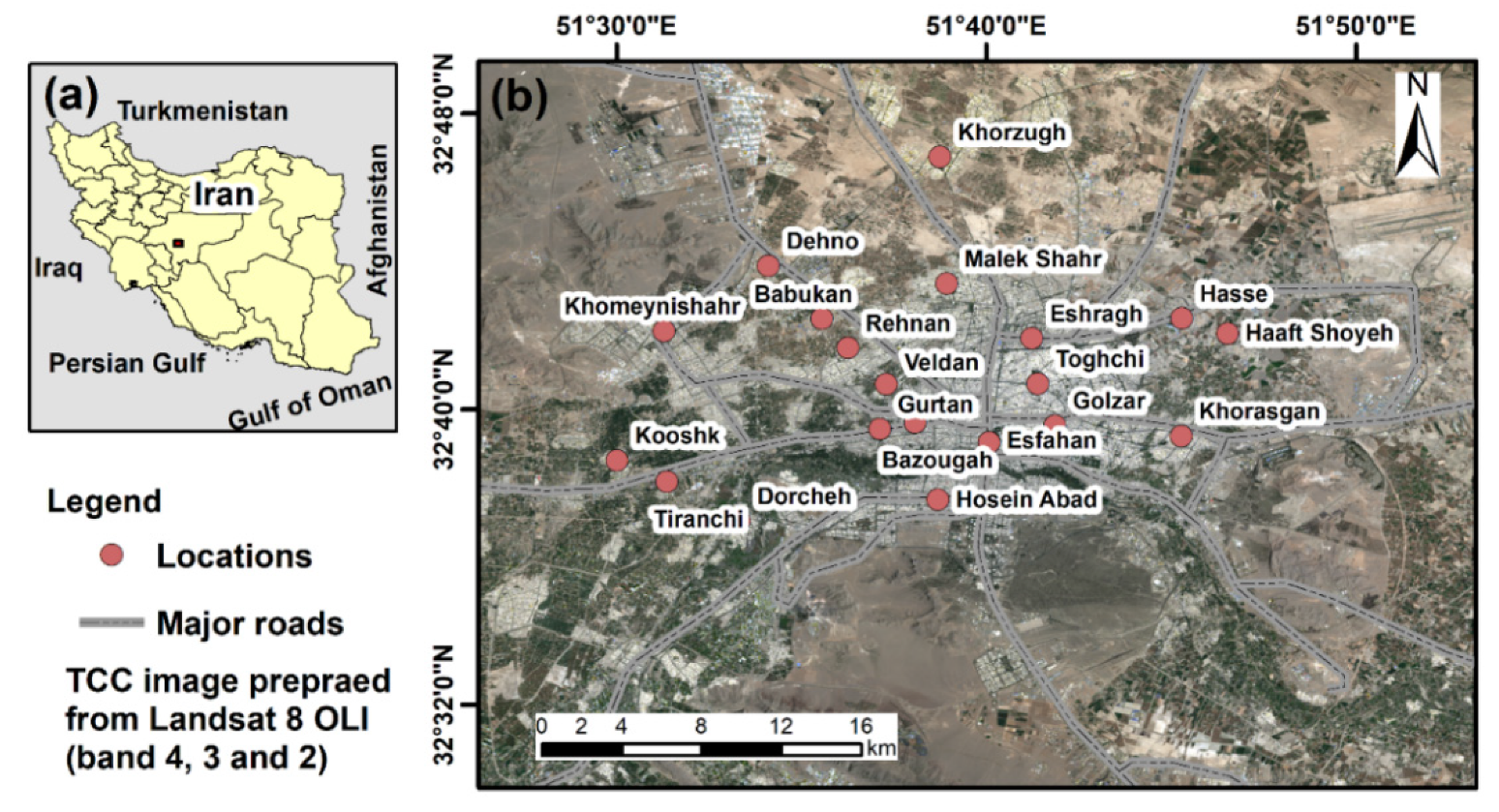
2. Study Area
3. Materials and Methods
3.1. Data Sources
3.2. Methods
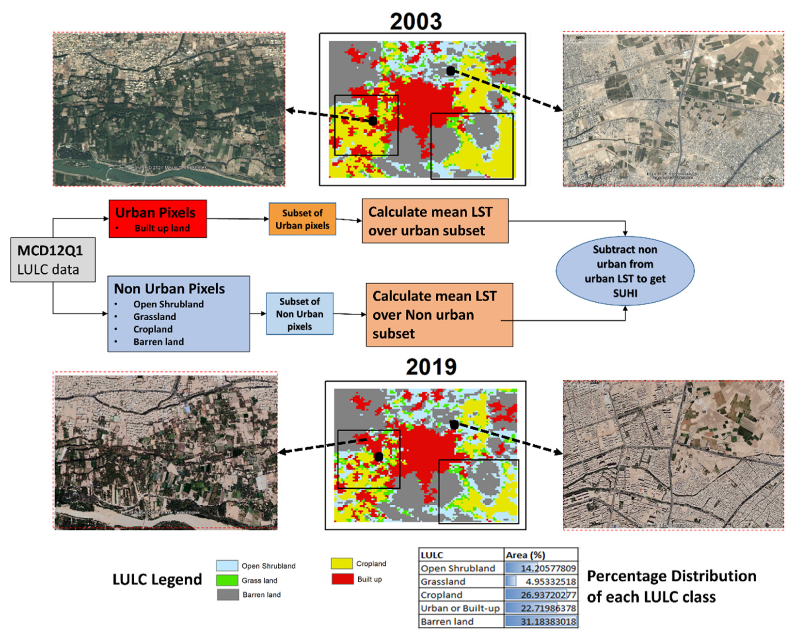
3.2.1. Definitions of Urban and Rural Regions
3.2.2. Surface Urban Heat Island Assessment
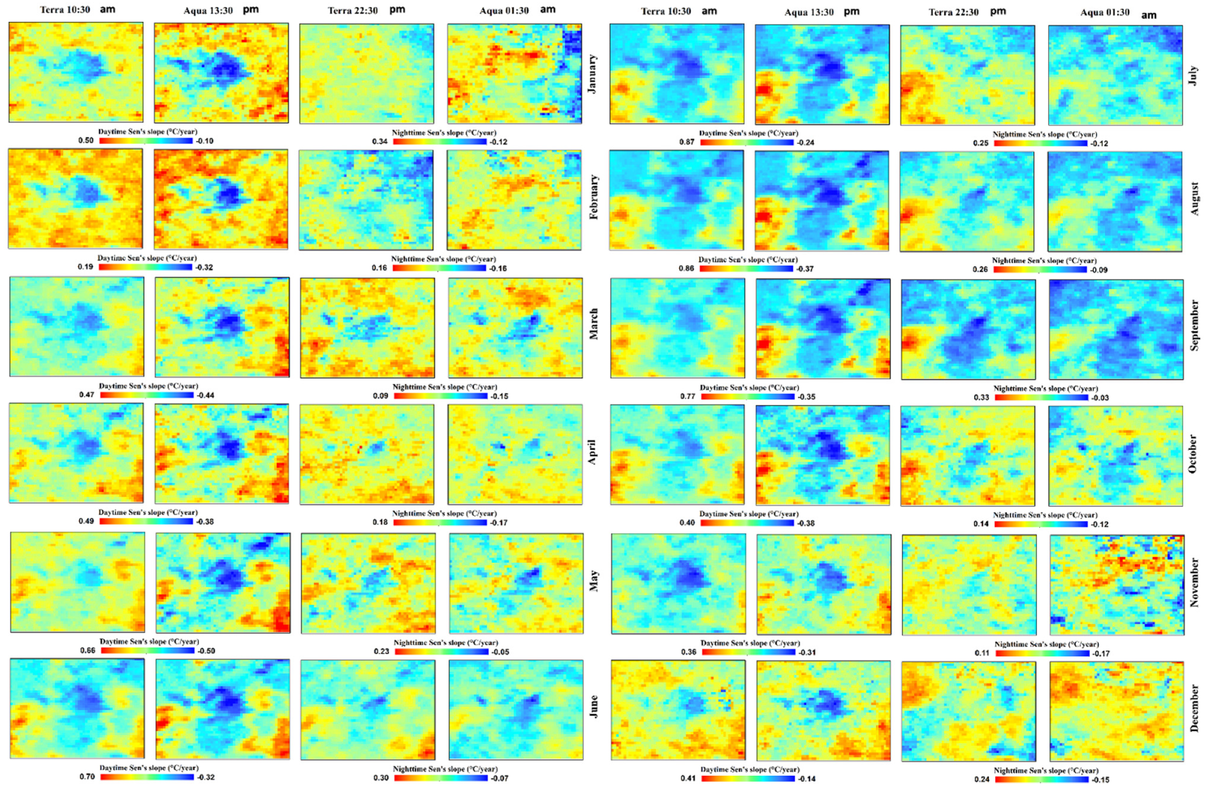
3.2.3. LST Trend Analysis Method
3.2.4. Exploring the SUHI Drivers
4. Results
4.1. Spatial Variation and Temporal Trend of LST
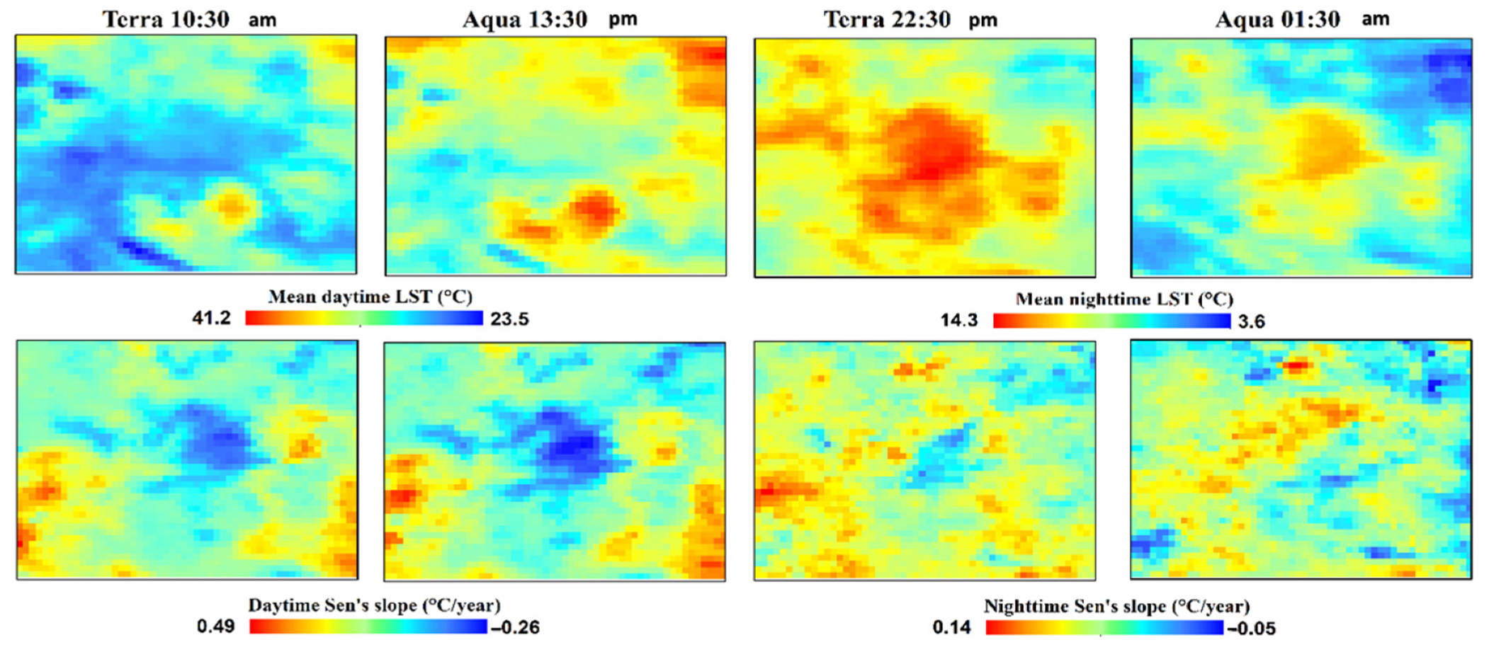
4.1.1. Annual Spatial Pattern of LST
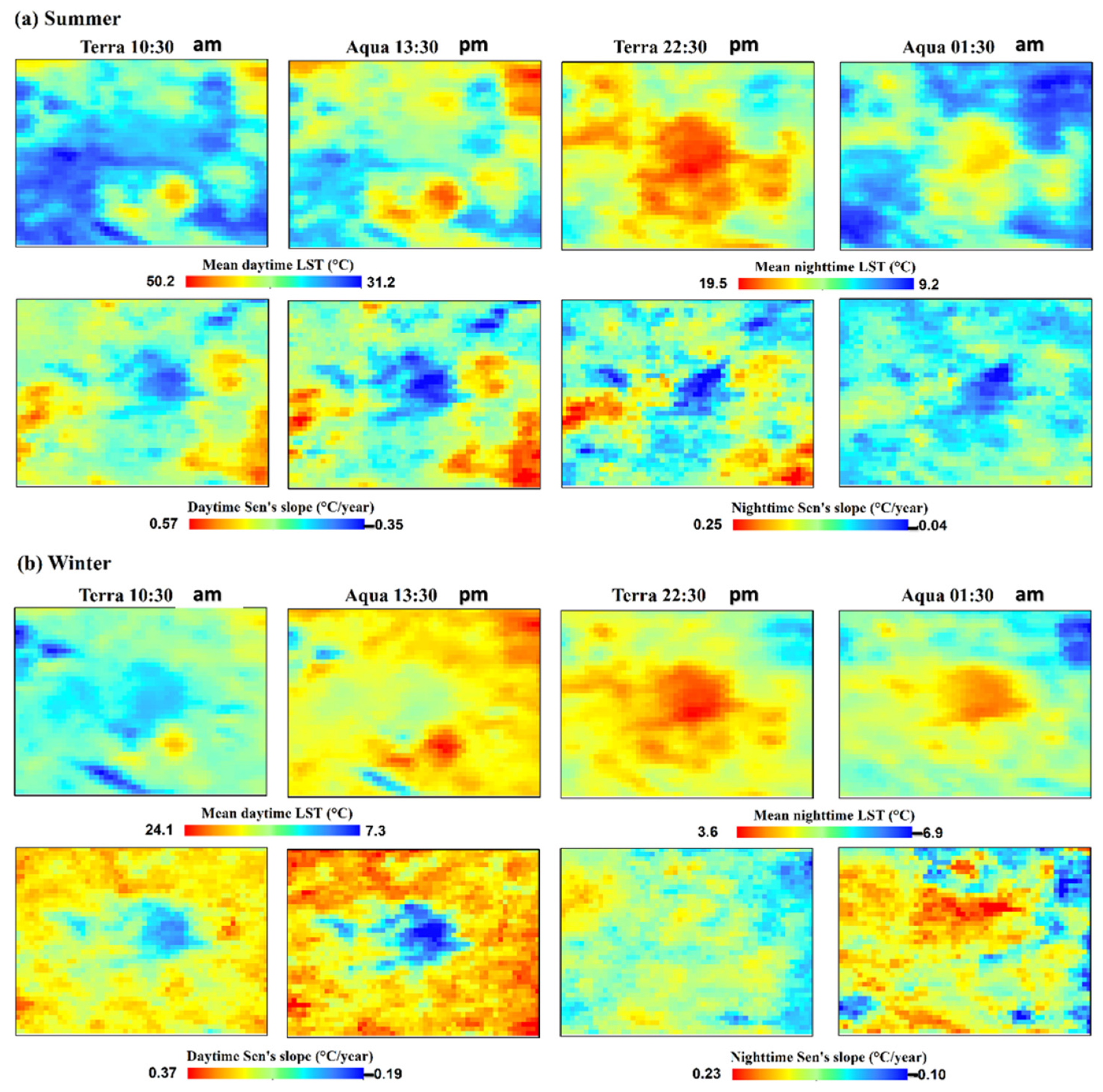
4.1.2. Seasonal Spatial Pattern of LST
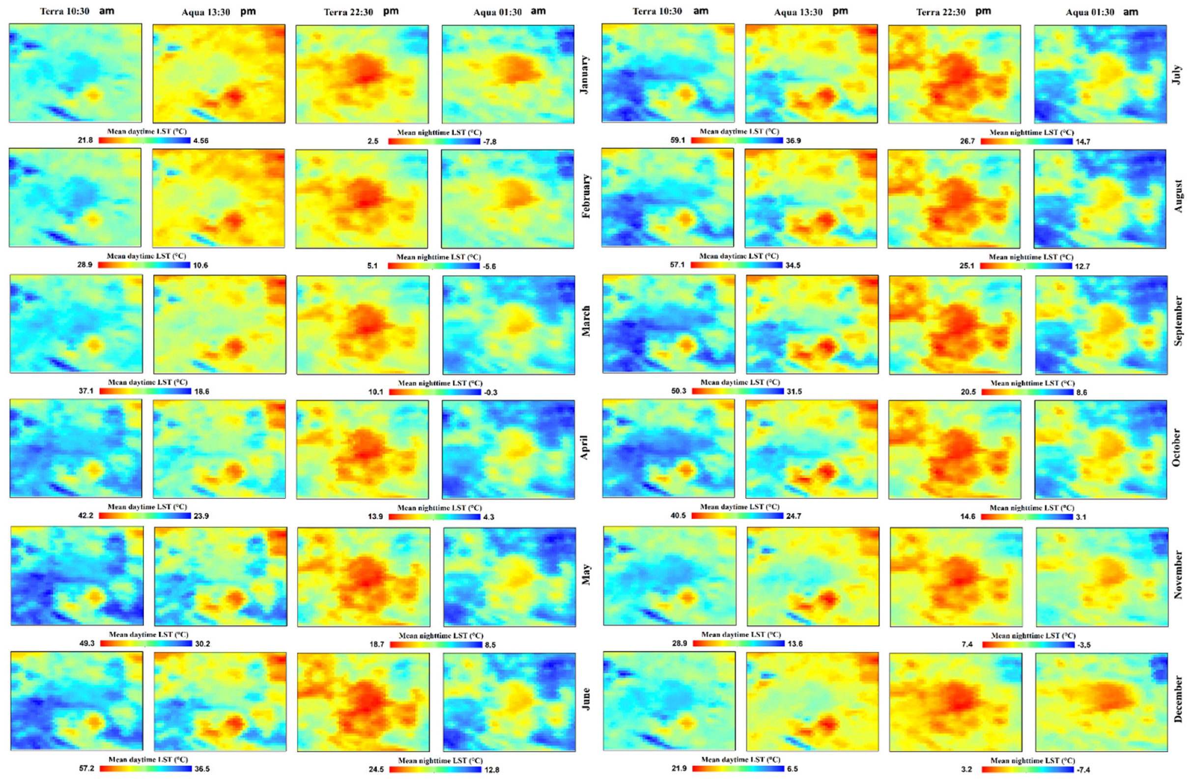
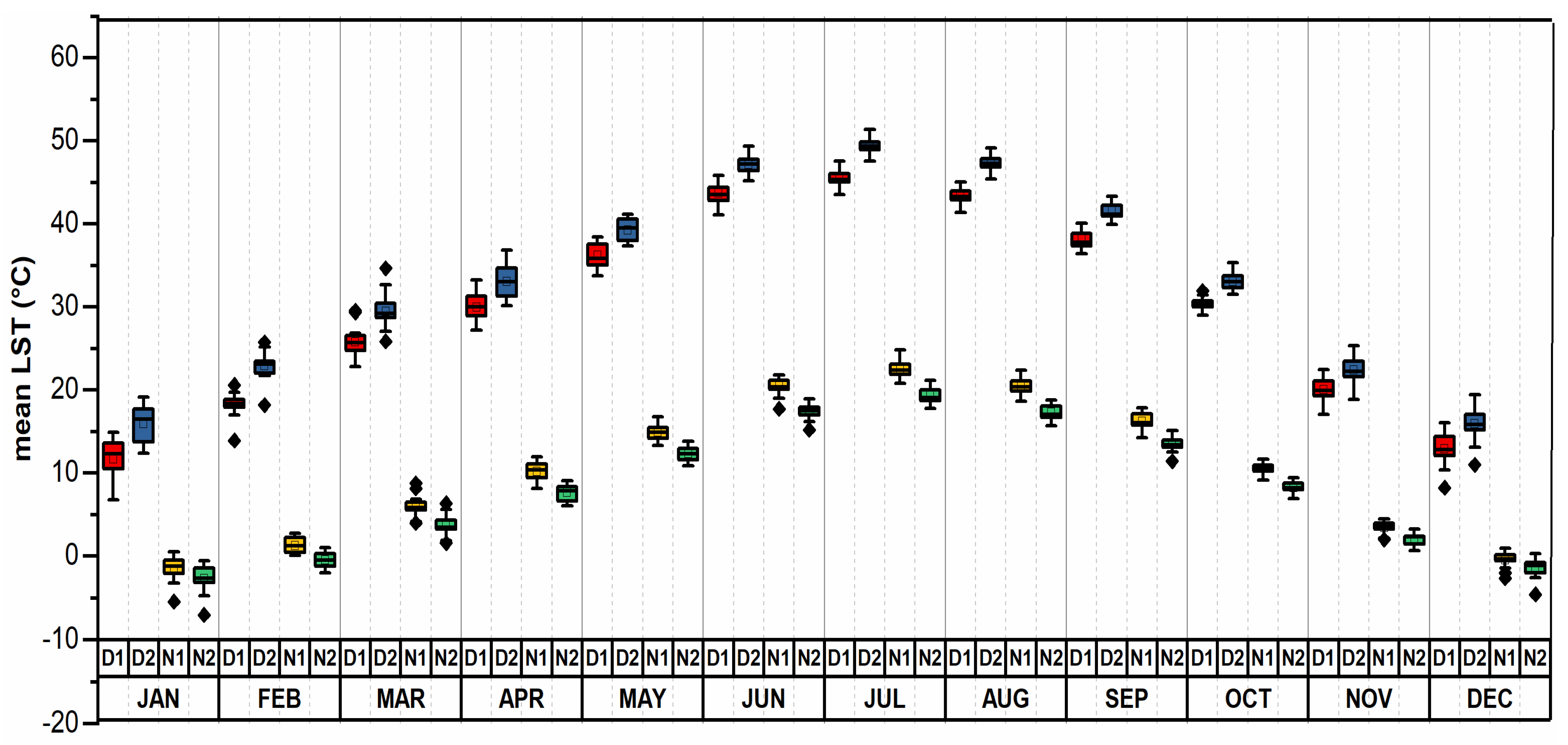
4.1.3. Monthly Spatial Pattern of LST
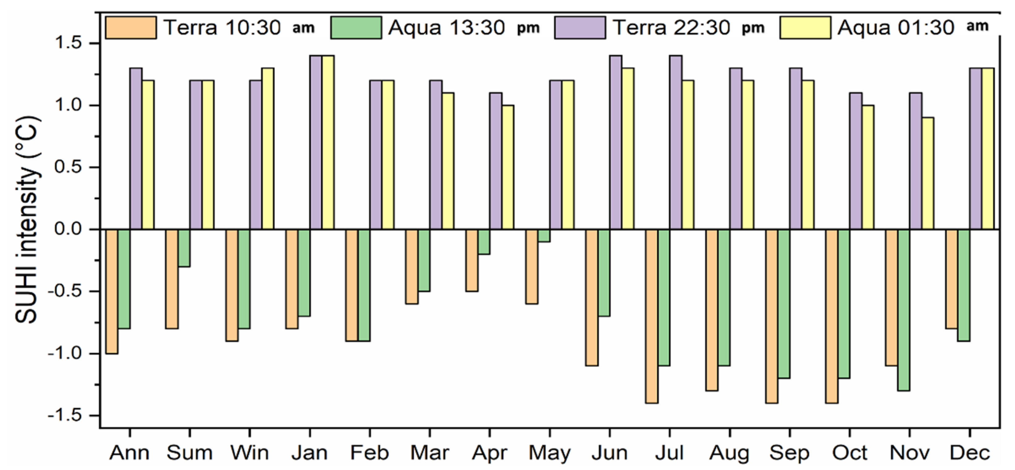
4.2. SUHI Intensity Variation
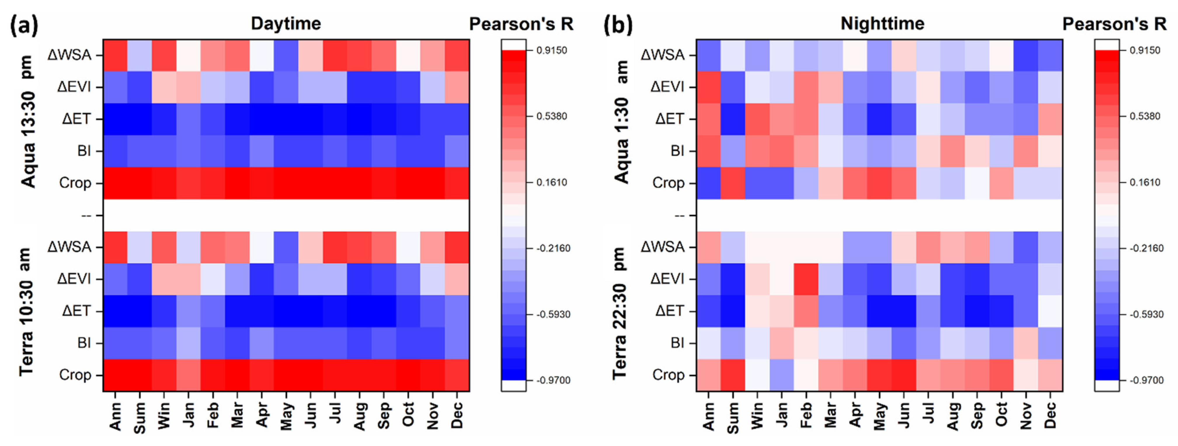
4.3. Relationships between the SUHI Intensity and Its Potential Influencing Factors
5. Discussion
5.1. Variations in the SUHI Intensity
5.2. The Effects of Each Factor on SUHI Intensity
6. Conclusions
Author Contributions
Funding
Institutional Review Board Statement
Informed Consent Statement
Data Availability Statement
Conflicts of Interest
Appendix A

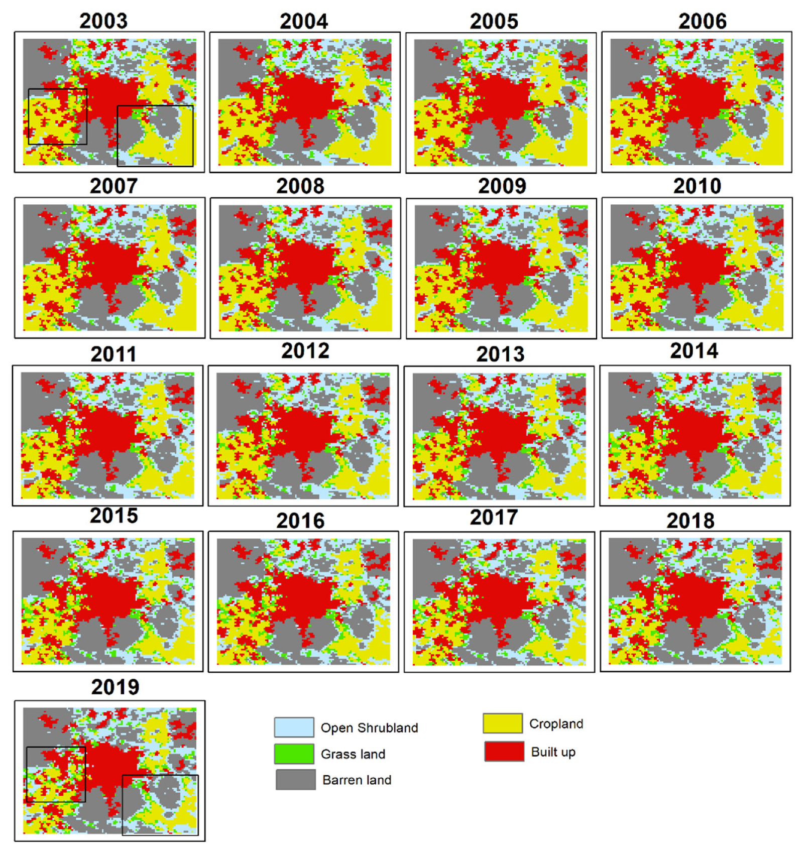
| LULC | 2003 | 2007 | 2011 | 2015 |
|---|---|---|---|---|
| Open Shrub land | 218.75 | 243.58 | 285.73 | 280.77 |
| Grassland | 76.27 | 75.10 | 80.81 | 102.34 |
| Cropland | 414.81 | 404.67 | 344.75 | 316.01 |
| Urban or Built-up | 319.86 | 326.46 | 339.53 | 350.55 |
| Barren land | 480.20 | 467.09 | 479.08 | 490.28 |

References
- Shen, H.; Huang, L.; Zhang, L.; Wu, P.; Zeng, C. Long-term and fi ne-scale satellite monitoring of the urban heat island effect by the fusion of multi-temporal and multi-sensor remote sensed data: A 26-year case study of the city of Wuhan in China. Remote Sens. Environ. 2016, 172, 109–125. [Google Scholar] [CrossRef]
- Sun, Y.; Zhao, S. Spatiotemporal dynamics of urban expansion in 13 cities across the Jing-Jin-Ji urban agglomeration from 1978 to 2015. Ecol. Indic. 2018, 87, 302–313. [Google Scholar] [CrossRef]
- Weng, Q.; Firozjaei, M.K.; Sedighi, A.; Kiavarz, M.; Alavipanah, S.K. Statistical analysis of surface urban heat island intensity variations: A case study of Babol city, Iran. GIScience Remote Sens. 2019, 56, 576–604. [Google Scholar] [CrossRef]
- Moonen, P.; Defraeye, T.; Dorer, V.; Blocken, B.; Carmeliet, J. Urban Physics: Effect of the micro-climate on comfort, health and energy demand. Front. Archit. Res. 2012, 1, 197–228. [Google Scholar] [CrossRef] [Green Version]
- Kikegawa, Y.; Genchi, Y.; Kondo, H.; Hanaki, K. Impacts of city-block-scale countermeasures against urban heat-island phenomena upon a building’s energy-consumption for air-conditioning. Appl. Energy 2006, 83, 649–668. [Google Scholar] [CrossRef]
- Li, Z.; Zhou, Y.; Wan, B.; Chen, Q.; Huang, B.; Cui, Y.; Chung, H. The impact of urbanization on air stagnation: Shenzhen as case study. Sci. Total Environ. 2019, 664, 347–362. [Google Scholar] [CrossRef] [PubMed]
- Liang, L.; Wang, Z.; Li, J. The effect of urbanization on environmental pollution in rapidly developing urban agglomerations. J. Clean. Prod. 2019, 237, 117649. [Google Scholar] [CrossRef]
- Uttara, S.; Bhuvandas, N.; Aggarwal, V. Impacts of urbanization on environment. Int. J. Res. Eng. Appl. Sci. 2012, 2, 1637–1645. [Google Scholar]
- Jeong, A.; Dorn, R.I. Soil erosion from urbanization processes in the Sonoran Desert, Arizona, USA. Land Degrad. Dev. 2019, 30, 226–238. [Google Scholar] [CrossRef]
- Malik, S.; Pal, S.C.; Sattar, A.; Singh, S.K.; Das, B.; Chakrabortty, R.; Mohammad, P. Trend of extreme rainfall events using suitable Global Circulation Model to combat the water logging condition in Kolkata Metropolitan Area. Urban Clim. 2020, 32, 100599. [Google Scholar] [CrossRef]
- Mbao, E.O.; Gao, J.; Wang, Y.; Sitoki, L.; Pan, Y.; Wang, B. Sensitivity and reliability of diatom metrics and guilds in detecting the impact of urbanization on streams. Ecol. Indic. 2020, 116, 106506. [Google Scholar] [CrossRef]
- Blair, R.B. Birds and butterflies along urban gradients in two ecoregions of the United States: Is urbanization creating a homogeneous fauna? In Biotic Homogenization; Springer: Berlin/Heidelberg, Germany, 2001; pp. 33–56. [Google Scholar]
- Fan, C.; Myint, S.W.; Kaplan, S.; Middel, A.; Zheng, B.; Rahman, A.; Huang, H.-P.; Brazel, A.; Blumberg, D.G. Understanding the impact of urbanization on surface urban heat islands—A longitudinal analysis of the oasis effect in subtropical desert cities. Remote Sens. 2017, 9, 672. [Google Scholar] [CrossRef] [Green Version]
- Zhou, D.; Xiao, J.; Bonafoni, S.; Berger, C.; Deilami, K.; Zhou, Y.; Frolking, S.; Yao, R.; Qiao, Z.; Sobrino, J.A. Satellite remote sensing of surface urban heat islands: Progress, challenges, and perspectives. Remote Sens. 2019, 11, 48. [Google Scholar] [CrossRef] [Green Version]
- Kim, H.H. Urban heat island. Int. J. Remote Sens. 1992, 13, 2319–2336. [Google Scholar] [CrossRef]
- Qiu, G.Y.; Zou, Z.; Li, X.; Li, H.; Guo, Q.; Yan, C.; Tan, S. Experimental studies on the effects of green space and evapotranspiration on urban heat island in a subtropical megacity in China. Habitat Int. 2017, 68, 30–42. [Google Scholar] [CrossRef]
- Qin, Y.; He, Y.; Hiller, J.E.; Mei, G. A new water-retaining paver block for reducing runoff and cooling pavement. J. Clean. Prod. 2018, 199, 948–956. [Google Scholar] [CrossRef]
- Mohajerani, A.; Bakaric, J.; Jeffrey-Bailey, T. The urban heat island effect, its causes, and mitigation, with reference to the thermal properties of asphalt concrete. J. Environ. Manag. 2017, 197, 522–538. [Google Scholar] [CrossRef]
- Du, H.; Wang, D.; Wang, Y.; Zhao, X.; Qin, F.; Jiang, H.; Cai, Y. Influences of land cover types, meteorological conditions, anthropogenic heat and urban area on surface urban heat island in the Yangtze River Delta Urban Agglomeration. Sci. Total Environ. 2016, 571, 461–470. [Google Scholar] [CrossRef] [PubMed]
- Stewart, I.; Oke, T.R. Newly developed “thermal climate zones” for defining and measuring urban heat island magnitude in the canopy layer. In Proceedings of the Eighth Symposium on Urban Environment, Phoenix, AZ, USA, 12 January 2009. [Google Scholar]
- Marando, F.; Salvatori, E.; Sebastiani, A.; Fusaro, L.; Manes, F. Regulating ecosystem services and green infrastructure: Assessment of urban heat island effect mitigation in the municipality of Rome, Italy. Ecol. Modell. 2019, 392, 92–102. [Google Scholar] [CrossRef]
- Hu, Y.; Hou, M.; Jia, G.; Zhao, C.; Zhen, X.; Xu, Y. Comparison of surface and canopy urban heat islands within megacities of eastern China. ISPRS J. Photogramm. Remote Sens. 2019, 156, 160–168. [Google Scholar]
- Zhang, X.; Zhong, T.; Feng, X.; Wang, K. Estimation of the relationship between vegetation patches and urban land surface temperature with remote sensing. Int. J. Remote Sens. 2009, 30, 2105–2118. [Google Scholar] [CrossRef]
- Kato, S.; Yamaguchi, Y. Estimation of storage heat flux in an urban area using ASTER data. Remote Sens. Environ. 2007, 110, 1–17. [Google Scholar] [CrossRef]
- Mirzaei, P.A.; Haghighat, F. Approaches to study urban heat island–abilities and limitations. Build. Environ. 2010, 45, 2192–2201. [Google Scholar] [CrossRef]
- Pichierri, M.; Bonafoni, S.; Biondi, R. Satellite air temperature estimation for monitoring the canopy layer heat island of Milan. Remote Sens. Environ. 2012, 127, 130–138. [Google Scholar] [CrossRef]
- Gaur, A.; Eichenbaum, M.K.; Simonovic, S.P. Analysis and modelling of surface Urban Heat Island in 20 Canadian cities under climate and land-cover change. J. Environ. Manag. 2018, 206, 145–157. [Google Scholar] [CrossRef] [PubMed]
- Voogt, J.A.; Oke, T.R. Thermal remote sensing of urban climates. Remote Sens. Environ. 2003, 86, 370–384. [Google Scholar] [CrossRef]
- Li, X.; Zhou, W.; Ouyang, Z. Relationship between land surface temperature and spatial pattern of greenspace: What are the effects of spatial resolution? Landsc. Urban Plan. 2013, 114, 1–8. [Google Scholar] [CrossRef]
- Li, X.; Zhou, Y.; Asrar, G.R.; Imhoff, M.; Li, X. The surface urban heat island response to urban expansion: A panel analysis for the conterminous United States. Sci. Total Environ. 2017, 605, 426–435. [Google Scholar] [CrossRef]
- Clinton, N.; Gong, P. MODIS detected surface urban heat islands and sinks: Global locations and controls. Remote Sens. Environ. 2013, 134, 294–304. [Google Scholar] [CrossRef]
- Heinl, M.; Hammerle, A.; Tappeiner, U.; Leitinger, G. Determinants of urban–rural land surface temperature differences—A landscape scale perspective. Landsc. Urban Plan. 2015, 134, 33–42. [Google Scholar] [CrossRef]
- Camilloni, I.; Barros, V. On the urban heat island effect dependence on temperature trends. Clim. Change 1997, 37, 665–681. [Google Scholar] [CrossRef]
- Li, L.; Zha, Y. Satellite-Based Spatiotemporal Trends of Canopy Urban Heat Islands and Associated Drivers in China’s 32 Major Cities. Remote Sens. 2019, 11, 102. [Google Scholar] [CrossRef] [Green Version]
- Yao, R.; Wang, L.; Huang, X.; Liu, Y.; Niu, Z.; Wang, S.; Wang, L. Long-term trends of surface and canopy layer urban heat island intensity in 272 cities in the mainland of China. Sci. Total Environ. 2021, 772, 145607. [Google Scholar] [CrossRef] [PubMed]
- Du, H.; Zhan, W.; Liu, Z.; Li, J.; Li, L.; Lai, J.; Miao, S.; Huang, F.; Wang, C.; Wang, C.; et al. Simultaneous investigation of surface and canopy urban heat islands over global cities. ISPRS J. Photogramm. Remote Sens. 2021, 181, 67–83. [Google Scholar] [CrossRef]
- Li, L.; Zha, Y.; Wang, R. Relationship of surface urban heat island with air temperature and precipitation in global large cities. Ecol. Indic. 2020, 117, 106683. [Google Scholar] [CrossRef]
- Oke, T.R. Canyon geometry and the nocturnal urban heat island: Comparison of scale model and field observations. J. Climatol. 1981, 1, 237–254. [Google Scholar] [CrossRef]
- Rizvi, S.H.; Fatima, H.; Iqbal, M.J.; Alam, K. The effect of urbanization on the intensification of SUHIs: Analysis by LULC on Karachi. J. Atmos. Solar-Terr. Phys. 2020, 207, 105374. [Google Scholar] [CrossRef]
- Tsou, J.; Zhuang, J.; Li, Y.; Zhang, Y. Urban Heat Island Assessment Using the Landsat 8 Data: A Case Study in Shenzhen and Hong Kong. Urban Sci. 2017, 1, 10. [Google Scholar] [CrossRef]
- Gohain, K.J.; Mohammad, P.; Goswami, A. Assessing the impact of land use land cover changes on land surface temperature over Pune city, India. Quat. Int. 2021, 575–576, 259–269. [Google Scholar] [CrossRef]
- Hung, T.; Uchihama, D.; Ochi, S.; Yasuoka, Y. Assessment with satellite data of the urban heat island effects in Asian mega cities. Int. J. Appl. Earth Obs. Geoinf. 2006, 8, 34–48. [Google Scholar] [CrossRef]
- Yang, Q.; Huang, X.; Tang, Q. The footprint of urban heat island effect in 302 Chinese cities: Temporal trends and associated factors. Sci. Total Environ. 2019, 655, 652–662. [Google Scholar] [CrossRef]
- Mohammad, P.; Goswami, A. Surface urban heat island variation over major Indian cities across different climatic zone. In Proceedings of the EGU General Assembly Conference Abstracts, 22nd EGU General Assembly, Online. 4–8 May 2020; p. 6444. Available online: https://ui.adsabs.harvard.edu/abs/2020EGUGA..22.6444M/abstract (accessed on 13 October 2021).
- Miles, V.; Esau, I. Seasonal and spatial characteristics of Urban Heat Islands (UHIs) in northern West Siberian cities. Remote Sens. 2017, 9, 989. [Google Scholar] [CrossRef] [Green Version]
- Schwarz, N.; Lautenbach, S.; Seppelt, R. Exploring indicators for quantifying surface urban heat islands of European cities with MODIS land surface temperatures. Remote Sens. Environ. 2011, 115, 3175–3186. [Google Scholar] [CrossRef]
- Mohammad, P.; Goswami, A.; Bonafoni, S. The Impact of the Land Cover Dynamics on Surface Urban Heat Island Variations in Semi-Arid Cities: A Case Study in Ahmedabad City, India, Using Multi-Sensor/Source Data. Sensors 2019, 19, 3701. [Google Scholar] [CrossRef] [Green Version]
- Yao, R.; Wang, L.; Huang, X.; Niu, Z.; Liu, F.; Wang, Q. Temporal trends of surface urban heat islands and associated determinants in major Chinese cities. Sci. Total Environ. 2017, 609, 742–754. [Google Scholar] [CrossRef] [PubMed]
- Ramamurthy, P.; Sangobanwo, M. Inter-annual variability in urban heat island intensity over 10 major cities in the United States. Sustain. Cities Soc. 2016, 26, 65–75. [Google Scholar] [CrossRef]
- Cao, C.; Lee, X.; Liu, S.; Schultz, N.; Xiao, W.; Zhang, M.; Zhao, L. Urban heat islands in China enhanced by haze pollution. Nat. Commun. 2016, 7, 1–7. [Google Scholar] [CrossRef]
- Yue, W.; Liu, X.; Zhou, Y.; Liu, Y. Impacts of urban configuration on urban heat island: An empirical study in China mega-cities. Sci. Total Environ. 2019, 671, 1036–1046. [Google Scholar] [CrossRef]
- Manoli, G.; Fatichi, S.; Schläpfer, M.; Yu, K.; Crowther, T.W.; Meili, N.; Burlando, P.; Katul, G.G.; Bou-Zeid, E. Magnitude of urban heat islands largely explained by climate and population. Nature 2019, 573, 55–60. [Google Scholar] [CrossRef] [PubMed]
- Peng, S.; Piao, S.; Ciais, P.; Friedlingstein, P.; Ottle, C.; Bréon, F.M.; Nan, H.; Zhou, L.; Myneni, R.B. Surface urban heat island across 419 global big cities. Environ. Sci. Technol. 2012, 46, 696–703. [Google Scholar] [CrossRef]
- Rasul, A.; Balzter, H.; Smith, C.; Remedios, J.; Adamu, B.; Sobrino, J.; Srivanit, M.; Weng, Q. A Review on Remote Sensing of Urban Heat and Cool Islands. Land 2017, 6, 38. [Google Scholar] [CrossRef] [Green Version]
- Mohammad, P.; Goswami, A. Quantifying diurnal and seasonal variation of surface urban heat island intensity and its associated determinants across different climatic zones over Indian cities. GIScience Remote Sens. 2021, 1–27. [Google Scholar] [CrossRef]
- Lazzarini, M.; Molini, A.; Marpu, P.R.; Ouarda, T.B.M.J.; Ghedira, H. Urban climate modifications in hot desert cities: The role of land cover, local climate, and seasonality. Geophys. Res. Lett. 2015, 42, 9980–9989. [Google Scholar] [CrossRef] [Green Version]
- Mirzaei, M.; Verrelst, J.; Arbabi, M.; Shaklabadi, Z.; Lotfizadeh, M. Urban heat island monitoring and impacts on citizen’s general health status in Isfahan metropolis: A remote sensing and field survey approach. Remote Sens. 2020, 12, 1350. [Google Scholar] [CrossRef]
- Shirani-Bidabadi, N.; Nasrabadi, T.; Faryadi, S.; Larijani, A.; Roodposhti, M.S. Evaluating the spatial distribution and the intensity of urban heat island using remote sensing, case study of Isfahan city in Iran. Sustain. Cities Soc. 2019, 45, 686–692. [Google Scholar] [CrossRef]
- Montazeri, M.; Masoodian, S.A. Tempo-Spatial Behavior of Surface Urban Heat Island of Isfahan Metropolitan Area. J. Indian Soc. Remote Sens. 2020, 48, 263–270. [Google Scholar] [CrossRef]
- Madanian, M.; Soffianian, A.R.; Soltani Koupai, S.; Pourmanafi, S.; Momeni, M. The study of thermal pattern changes using Landsat-derived land surface temperature in the central part of Isfahan province. Sustain. Cities Soc. 2018, 39, 650–661. [Google Scholar] [CrossRef]
- Ramezankhani, R.; Sajjadi, N.; Jozi, S.A.; Shirzadi, M.R. Climate and environmental factors affecting the incidence of cutaneous leishmaniasis in Isfahan, Iran. Environ. Sci. Pollut. Res. 2018, 25, 11516–11526. [Google Scholar] [CrossRef]
- Kottek, M.; Grieser, J.; Beck, C.; Rudolf, B.; Rubel, F. World map of the Köppen-Geiger climate classification updated. Meteorol. Z. 2006, 15, 259–263. [Google Scholar] [CrossRef]
- Eslamian, S.S.; Feizi, H. Maximum monthly rainfall analysis using L-moments for an arid region in Isfahan province, Iran. J. Appl. Meteorol. Climatol. 2007, 46, 494–503. [Google Scholar] [CrossRef]
- Bihamta, N.; Soffianian, A.; Fakheran, S.; Gholamalifard, M. Using the SLEUTH urban growth model to simulate future urban expansion of the Isfahan metropolitan area, Iran. J. Indian Soc. Remote Sens. 2015, 43, 407–414. [Google Scholar] [CrossRef]
- Abbasnia, M.; Tavousi, T.; Khosravi, M.; Toros, H. Investigation of interactive effects between temperature trend and urban climate during the last decades: A case study of Isfahan-Iran. Eur. J. Sci. Technol. 2016, 4, 74–81. [Google Scholar]
- Wan, Z. A generalized split-window algorithm for retrieving land-surface temperature from space. IEEE Trans. Geosci. Remote Sens. 1996, 34, 892–905. [Google Scholar] [CrossRef] [Green Version]
- Wan, Z. New refinements and validation of the collection-6 MODIS land-surface temperature/emissivity product. Remote Sens. Environ. 2014, 140, 36–45. [Google Scholar] [CrossRef]
- Senay, G.B.; Budde, M.E.; Verdin, J.P. Enhancing the Simplified Surface Energy Balance (SSEB) approach for estimating landscape ET: Validation with the METRIC model. Agric. Water Manag. 2011, 98, 606–618. [Google Scholar] [CrossRef]
- Bastiaanssen, W.G.M.G.M.; Menenti, M.; Feddes, R.A.; Holtslag, A.A.M.; Pelgrum, H.; Wang, J.; Ma, Y.; Moreno, J.F.; Roerink, G.J.; Van der Wal, T.; et al. A remote sensing surface energy balance algorithm for land (SEBAL): 1. Formulation. J. Hydrol. 1998, 212–213, 198–212. [Google Scholar] [CrossRef]
- Gowda, P.H.; Chävez, J.; Howell, T.A.; Marek, T.H.; New, L.L. Surface energy balance based evapotranspiration mapping in the Texas high plains. Sensors 2008, 8, 5186–5201. [Google Scholar] [CrossRef]
- Chakraborty, T.; Lee, X. A simplified urban-extent algorithm to characterize surface urban heat islands on a global scale and examine vegetation control on their spatiotemporal variability. Int. J. Appl. Earth Obs. Geoinf. 2019, 74, 269–280. [Google Scholar] [CrossRef]
- Chakraborty, T.; Hsu, A.; Manya, D.; Sheriff, G. A spatially explicit surface urban heat island database for the United States: Characterization, uncertainties, and possible applications. ISPRS J. Photogramm. Remote Sens. 2020, 168, 74–88. [Google Scholar] [CrossRef]
- Mann, H.B. Nonparametric Tests Against Trend. Econometrica 1945, 13, 245–259. [Google Scholar] [CrossRef]
- Zhang, T.; Peng, J.; Liang, W.; Yang, Y.; Liu, Y. Spatial-temporal patterns of water use efficiency and climate controls in China’s Loess Plateau during 2000–2010. Sci. Total Environ. 2016, 565, 105–122. [Google Scholar] [CrossRef]
- Radhakrishnan, K.; Sivaraman, I.; Jena, S.K.; Sarkar, S.; Adhikari, S. A Climate Trend Analysis of Temperature and Rainfall in India. Clim. Chang. Environ. Sustain. 2017, 5, 146. [Google Scholar] [CrossRef]
- Araghi, A.; Mousavi Baygi, M.; Adamowski, J.; Malard, J.; Nalley, D.; Hasheminia, S.M. Using wavelet transforms to estimate surface temperature trends and dominant periodicities in Iran based on gridded reanalysis data. Atmos. Res. 2015, 155, 52–72. [Google Scholar] [CrossRef]
- Zhao, W.; He, J.; Wu, Y.; Xiong, D.; Wen, F.; Li, A. An Analysis of Land Surface Temperature Trends in the Central Himalayan Region Based on MODIS Products. Remote Sens. 2019, 11, 900. [Google Scholar] [CrossRef] [Green Version]
- Mohammad, P.; Goswami, A. Temperature and precipitation trend over 139 major Indian cities: An assessment over a century. Model. Earth Syst. Environ. 2019, 5, 1481–1493. [Google Scholar] [CrossRef]
- Sen, K.P. Estimates of the Regression Coefficient Based on Kendall’ s Tau Pranab Kumar Sen. J. Am. Stat. Assoc. 1968, 63, 1379–1389. [Google Scholar] [CrossRef]
- Madanian, M.; Soffianian, A.R.; Koupai, S.S.; Pourmanafi, S.; Momeni, M. Analyzing the effects of urban expansion on land surface temperature patterns by landscape metrics: A case study of Isfahan city, Iran. Environ. Monit. Assess. 2018, 190, 189. [Google Scholar] [CrossRef]
- Wheeler, S.M.; Abunnasr, Y.; Dialesandro, J.; Assaf, E.; Agopian, S.; Gamberini, V.C. Mitigating Urban Heating in Dryland Cities: A Literature Review. J. Plan. Lit. 2019, 34, 434–446. [Google Scholar] [CrossRef]
- Peel, M.C.; Finlayson, B.L.; McMahon, T.A. Updated world map of the Koppen-Geiger climate classification. Hydrol. Earth Syst. Sci. 2007, 11, 1633–1644. [Google Scholar] [CrossRef] [Green Version]
- Zhou, D.; Zhao, S.; Zhang, L.; Sun, G.; Liu, Y. The footprint of urban heat island effect in China. Sci. Rep. 2015, 5, 2–12. [Google Scholar] [CrossRef]
- Hawkins, T.W.; Brazel, A.J.; Stefanov, W.L.; Bigler, W.; Saffell, E.M. The Role of Rural Variability in Urban Heat Island Determination for Phoenix, Arizona. J. Appl. Meteorol. 2004, 43, 476–486. [Google Scholar] [CrossRef]
- Mohammad, P.; Goswami, A. Spatial variation of surface urban heat island magnitude along the urban-rural gradient of four rapidly growing Indian cities. Geocarto Int. 2021, 1–23. [Google Scholar] [CrossRef]
- Shastri, H.; Barik, B.; Ghosh, S.; Venkataraman, C.; Sadavarte, P. Flip flop of Day-night and Summer-Winter Surface Urban Heat Island Intensity in India. Sci. Rep. 2017, 7, 1–8. [Google Scholar] [CrossRef] [Green Version]
- Kumar, R.; Mishra, V.; Buzan, J.; Kumar, R.; Shindell, D.; Huber, M. Dominant control of agriculture and irrigation on urban heat island in India. Sci. Rep. 2017, 7, 1–10. [Google Scholar] [CrossRef]
- Wu, X.; Wang, G.; Yao, R.; Wang, L.; Yu, D.; Gui, X. Investigating Surface Urban Heat Islands in South America Based on MODIS Data from 2003–2016. Remote Sens. 2019, 11, 1212. [Google Scholar] [CrossRef] [Green Version]
- Lazzarini, M.; Marpu, P.R.; Ghedira, H. Temperature-land cover interactions: The inversion of urban heat island phenomenon in desert city areas. Remote Sens. Environ. 2013, 130, 136–152. [Google Scholar] [CrossRef]
- Georgescu, M.; Moustaoui, M.; Mahalov, A.; Dudhia, J. An alternative explanation of the semiarid urban area “oasis effect”. J. Geophys. Res. Atmos. 2011, 116, 1–13. [Google Scholar] [CrossRef]
- Zhou, D.; Zhao, S.; Liu, S.; Zhang, L.; Zhu, C. Surface urban heat island in China’s 32 major cities: Spatial patterns and drivers. Remote Sens. Environ. 2014, 152, 51–61. [Google Scholar] [CrossRef]
- Arnfield, A.J. Two decades of urban climate research: A review of turbulence, exchanges of energy and water, and the urban heat island. Int. J. Climatol. 2003, 23, 1–26. [Google Scholar] [CrossRef]
- Mohammad, P.; Aghlmand, S.; Fadaei, A.; Gachkar, S.; Gachkar, D.; Karimi, A. Evaluating the role of the albedo of material and vegetation scenarios along the urban street canyon for improving pedestrian thermal comfort outdoors. Urban Clim. 2021, 40, 100993. [Google Scholar] [CrossRef]
- Hu, Y.; Jia, G. Influence of land use change on urban heat island derivedfrom multi-sensor data. Int. J. Climatol. 2010, 30, 1382–1395. [Google Scholar] [CrossRef]
- Gachkar, D.; Taghvaei, S.H.; Norouzian-Maleki, S. Outdoor Thermal Comfort Enhancement using Various Vegetation Species and Materials (Case study: Delgosha Garden, Iran). Sustain. Cities Soc. 2021, 75, 103309. [Google Scholar] [CrossRef]
- Karimi, A.; Sanaieian, H.; Farhadi, H.; Norouzian-Maleki, S. Evaluation of the thermal indices and thermal comfort improvement by different vegetation species and materials in a medium-sized urban park. Energy Rep. 2020, 6, 1670–1684. [Google Scholar] [CrossRef]
- Zhou, D.; Bonafoni, S.; Zhang, L.; Wang, R. Remote sensing of the urban heat island effect in a highly populated urban agglomeration area in East China. Sci. Total Environ. 2018, 628–629, 415–429. [Google Scholar] [CrossRef] [PubMed]


| Terra 10:30 a.m. | Aqua 13:30 p.m. | Terra 22:30 p.m. | Aqua 01:30 a.m. | ||
|---|---|---|---|---|---|
| Annual | Non-Urban Pixels | 29.9 ± 2.3 | 33.4 ± 2.5 | 10.1 ± 1.3 | 8 ± 1.4 |
| Urban Pixels | 28.9 ± 1.9 | 32.6 ± 2 | 11.4 ± 1.7 | 9.2 ± 1.9 | |
| Summer | Non-Urban Pixels | 37.4 ± 3 | 40.5 ± 3.2 | 15.4 ± 1.4 | 12.6 ± 1.6 |
| Urban Pixels | 36.6 ± 2.3 | 40.2 ± 2.5 | 16.6 ± 1.7 | 13.8 ± 1.9 | |
| Winter | Non-Urban Pixels | 14.5 ± 1.6 | 18.5 ± 1.8 | −0.5 ± 1.1 | −1.8 ± 1.1 |
| Urban Pixels | 13.6 ± 1.3 | 17.7 ± 1.5 | 0.7 ± 1.6 | −0.5 ± 1.8 | |
| Jane | Non-Urban Pixels | 11.9 ± 1.6 | 16.1 ± 1.8 | −1.9 ± 1.2 | −3 ± 1.2 |
| Urban Pixels | 11.1 ± 1.2 | 15.4 ± 1.4 | −0.5 ± 1.7 | −1.6 ± 1.8 | |
| February | Non-Urban Pixels | 18.4 ± 1.9 | 23.1 ± 1.9 | 1 ± 1.1 | −0.7 ± 1.1 |
| Urban Pixels | 17.5 ± 1.6 | 22.2 ± 1.6 | 2.2 ± 1.6 | 0.5 ± 1.7 | |
| March | Non-Urban Pixels | 25.9 ± 2 | 29.6 ± 2.1 | 5.7 ± 1.1 | 3.4 ± 1.2 |
| Urban Pixels | 25.3 ± 1.5 | 29 ± 1.6 | 6.9 ± 1.6 | 4.5 ± 1.7 | |
| April | Non-Urban Pixels | 30.1 ± 2.4 | 33.1 ± 2.5 | 9.9 ± 1.2 | 7.4 ± 1.3 |
| Urban Pixels | 29.6 ± 1.8 | 32.9 ± 1.9 | 11 ± 1.5 | 8.4 ± 1.7 | |
| May | Non-Urban Pixels | 36.3 ± 3.2 | 39.2 ± 3.3 | 14.7 ± 1.4 | 12 ± 1.5 |
| Urban Pixels | 35.7 ± 2.4 | 39.1 ± 2.6 | 15.9 ± 1.6 | 13.2 ± 1.8 | |
| June | Non-Urban Pixels | 43.9 ± 3.5 | 47.3 ± 3.6 | 20.1 ± 1.7 | 17 ± 1.9 |
| Urban Pixels | 42.8 ± 2.8 | 46.6 ± 2.9 | 21.5 ± 1.8 | 18.3 ± 2.1 | |
| July | Non-Urban Pixels | 45.8 ± 3.5 | 49.6 ± 3.7 | 22.2 ± 1.7 | 19 ± 1.9 |
| Urban Pixels | 44.4 ± 3 | 48.5 ± 3.1 | 23.6 ± 1.8 | 20.2 ± 2.2 | |
| August | Non-Urban Pixels | 43.6 ± 3.6 | 47.5 ± 3.9 | 20.1 ± 1.9 | 17 ± 2.1 |
| Urban Pixels | 42.3 ± 3 | 46.4 ± 3.2 | 21.4 ± 2 | 18.2 ± 2.3 | |
| September | Non-Urban Pixels | 38.4 ± 3.2 | 41.8 ± 3.4 | 15.9 ± 1.9 | 13.2 ± 2.2 |
| Urban Pixels | 37 ± 2.7 | 40.6 ± 2.8 | 17.2 ± 2.1 | 14.4 ± 2.3 | |
| October | Non-Urban Pixels | 30.7 ± 2.5 | 33.3 ± 2.5 | 10.3 ± 1.7 | 8 ± 1.9 |
| Urban Pixels | 29.3 ± 2.2 | 32.1 ± 2.2 | 11.4 ± 1.9 | 9 ± 2.1 | |
| November | Non-Urban Pixels | 20.3 ± 1.7 | 22.7 ± 1.9 | 3.2 ± 1.3 | 1.8 ± 1.2 |
| Urban Pixels | 19.2 ± 1.6 | 21.4 ± 1.7 | 4.3 ± 1.7 | 2.7 ± 1.7 | |
| December | Non-Urban Pixels | 13.1 ± 1.5 | 16.2 ± 1.7 | −0.8 ± 1.2 | −1.7 ± 1.2 |
| Urban Pixels | 12.3 ± 1.2 | 15.3 ± 1.5 | 0.5 ± 1.7 | −0.4 ± 1.8 |
Publisher’s Note: MDPI stays neutral with regard to jurisdictional claims in published maps and institutional affiliations. |
© 2021 by the authors. Licensee MDPI, Basel, Switzerland. This article is an open access article distributed under the terms and conditions of the Creative Commons Attribution (CC BY) license (https://creativecommons.org/licenses/by/4.0/).
Share and Cite
Karimi, A.; Mohammad, P.; Gachkar, S.; Gachkar, D.; García-Martínez, A.; Moreno-Rangel, D.; Brown, R.D. Surface Urban Heat Island Assessment of a Cold Desert City: A Case Study over the Isfahan Metropolitan Area of Iran. Atmosphere 2021, 12, 1368. https://0-doi-org.brum.beds.ac.uk/10.3390/atmos12101368
Karimi A, Mohammad P, Gachkar S, Gachkar D, García-Martínez A, Moreno-Rangel D, Brown RD. Surface Urban Heat Island Assessment of a Cold Desert City: A Case Study over the Isfahan Metropolitan Area of Iran. Atmosphere. 2021; 12(10):1368. https://0-doi-org.brum.beds.ac.uk/10.3390/atmos12101368
Chicago/Turabian StyleKarimi, Alireza, Pir Mohammad, Sadaf Gachkar, Darya Gachkar, Antonio García-Martínez, David Moreno-Rangel, and Robert D. Brown. 2021. "Surface Urban Heat Island Assessment of a Cold Desert City: A Case Study over the Isfahan Metropolitan Area of Iran" Atmosphere 12, no. 10: 1368. https://0-doi-org.brum.beds.ac.uk/10.3390/atmos12101368