Quantifying the Impact of Future Climate Change on Runoff in the Amur River Basin Using a Distributed Hydrological Model and CMIP6 GCM Projections

Abstract

The Amur River is one of the top ten longest rivers in the world, and its hydrological response to future climate change has been rarely investigated. In this study, the outputs of four GCMs in the Coupled Model Intercomparison Project Phase 6 (CMIP6) were corrected and downscaled to drive a distributed hydrological model. Then, the spatial variations of runoff changes under the future climate conditions in the Amur River Basin were quantified. The results suggest that runoffs will tend to increase in the future period (2021–2070) compared with the baseline period (1961–2010), particularly in August and September. Differences were also found among different GCMs and scenarios. The ensemble mean of the GCMs suggests that the basin-averaged annual precipitation will increase by 14.6% and 15.2% under the SSP2-4.5 and SSP5-8.5 scenarios, respectively. The increase in the annual runoff under the SSP2-4.5 scenario (22.5%) is projected to be larger than that under the SSP5-8.5 scenario (19.2%) at the lower reach of the main channel. Future climate changes also tend to enhance the flood peak and flood volume. The findings of this study bring new understandings of the hydrological response to future climate changes and are helpful for water resource management in Eurasia.

1. Introduction

According to the sixth assessment report of IPCC, the warming of the surface temperature in the past 20 years (2001–2020) was about 0.99 °C compared with the pre-industrial revolution [1]. Rising air temperatures lead to increases in the atmosphere vapor holding capacity and changes in the precipitation frequency and intensity. These changes will significantly affect the hydrological cycle, which further influences water supplies on the local, regional and global scales [2], with potentially powerful effects on the runoff mechanisms [3,4] and natural disasters such as floods [5]. Particularly, the impact of climate change on runoffs receives relatively more attention due to its close relationship with the agriculture, hydropower, tourism and ecology around rivers [6]. Therefore, quantifying the effects of climate change on hydrological processes and runoffs are very important for water resources management and are helpful for decision-makers to develop adaptions to climate change.

Located in a high-latitude region, the Amur River is one of the top ten longest rivers in the world. With a large basin area and cold climate, the hydrological observations in the Amur River basin are limited. Therefore, compared with other large river basins in the world, the hydrological changes in the Amur River Basin have been less investigated. Particularly, the response of runoffs to future climate changes has been poorly understood. Previous studies have examined the trends in the precipitation and air temperature in the Amur River Basin to assess the patterns of regional climate change. Yu et al. [7] found that the annual air temperature in the Amur River Basin increased significantly from 1950 to 2010 based on an analysis of observations. This warming trend was also supported by Sun et al. [8] through investigating the observations in the Songhua Subbasin of the Amur River Basin. Yu et al. [7] revealed that the annual precipitation changed significantly in the lower reaches of the Amur River from 1950 to 2010. Precipitation and temperature changes in this basin may have a certain influence on the hydrological process. Zhou et al. [9] argued that precipitation and temperature in the summer were the main climatic factors affecting the hydrological processes in this basin. Bolgov et al. [10] found that the major floods in the Amur River Basin in 2013 were primarily caused by large areas covered by the extreme precipitation and the long durations of extreme events. Some studies have projected future climate changes in the Amur River Basin. Yang et al. [11] found that the air temperature in Northeast China will increase by 2.9 °C and 5.8 °C by the end of the 21st century under the SSP2-4.5 and SSP5-8.5 scenarios provided by CMIP6, respectively, and the precipitation will increase by 20–35% under the SSP5-8.5 scenario. Shin and Jung [12] used 34 GCMs from CMIP5 to analyze the future changes in the air temperature and precipitation in Northeast Asia, and they found that the increasing rates of air temperature and precipitation in the study basin were higher than the global averaged values. Although these above studies projected significant climate changes in the Amur River Basin, few studies have evaluated the hydrological response to future climate changes in this basin.

The development of hydrological and atmospheric models provides opportunities to study the hydrological effects of climate change on the regional scale [13]. For large watersheds, due to the great complexity and heterogeneity in topography, land use and climatology [14], the response of hydrological processes to climate change has significant spatial variations. The distributed hydrological model can better consider spatial heterogeneity by dividing watersheds into grids with independent inputs, boundary conditions and watershed characteristics [13,15]. Therefore, the distributed hydrological model is a powerful tool for assessing and analyzing the climate change impact [16]. In previous studies, distributed hydrological models have been validated and applied for climate change impact studies at some large river basins. Huang et al. [17] combined a large-scale hydrological model and the dynamic downscaling results of two global climate models provided by the CMIP5 and suggested a reduction in the annual runoff of the Upper Yangtze River in the future climate. Guimberteau et al. [18] used three hydrological models driven by the output by three GCMs provided by IPCC AR4 to analyze the future hydrological changes in the Amazon River Basin and found a general increase in runoff and precipitation by 2100. Zhang et al. [19] investigated the effects of future climate changes on extreme flows in the Upper Yellow River based on the hydrological models forced by four GCMs in CMIP5 and projected a significant change in the high flows. Although some hydrological model simulations in the Songhua Subbasin of the Amur River Basin have been reported in previous studies [20,21], systematic hydrological modeling of the whole Amur River Basin has rarely been studied. Most of the studies mentioned above used the CMIP5 projections, but few studies have evaluated the hydrological changes using the recently released CMIP6 model projections.

Therefore, in this study, a distributed hydrological model GBHM-HLJ was used to quantify the changes in the runoff in the Amur River Basin under two future climate scenarios, SSP2-4.5 and SSP5-8.5, using the downscaled and bias-corrected results of four GCMs provided by the CMIP6. The period from 1961 to 2010 was defined as the baseline period, and the period of 2021 to 2070 was taken as the future period. The main research objectives were: (1) to analyze the changes in precipitation and air temperature under the future climate scenarios, (2) evaluate the response of annual and seasonal runoffs to future climate changes and (3) assess the impact of future climate changes on floods.

2. Study Area and Data

The Amur River Basin is located in the northeastern part of Eurasia, with a basin area of 889,000 km². The Amur River has two sources: one is the Erguna River in the south, located in the Inner Mongolia Autonomous Region, and the other is the Shilka River in the north, originating in the Outer Hinggan Mountains. Originating from the Kluren Stream of the Erguna River, with a total length of 5498 km, the Amur River ranks the sixth-longest river in the world [22,23]. The topography of the Amur River Basin is characterized by high mountains in the west and gentle hills and low plains with extensive pastures in the east (Figure 1). The elevation of this basin ranges from 0 to 2485 m. The basin is located in the cold temperate zone and temperate zone, influenced by a monsoon climate. The main vegetation types in the study area are farmland, forest and grassland [24]. In this basin, the annual precipitation mainly concentrates in June–September, and the precipitation in these months accounts for 70% of the annual precipitation [25]. At the same time, the precipitation distribution in this basin changes gradually with the topography and the distance from the ocean. From the plain to the mountain area, the precipitation enhances with the increase of the elevation. From east to west, the precipitation decreases with the increasing distance from the ocean [26].

The data used in this study include the atmospheric forcing, the land surface data for the hydrological model simulation and the output data of the GCM. The atmospheric forcing data includes the daily air pressure, air temperature, precipitation, relative humidity, wind speed and sunshine hours observed at the meteorological stations. The data observed at the meteorological stations in China were obtained from the dataset of China’s terrestrial climate information (V3.0) provided by the China Meteorological Administration (http://data.cma.cn/, accessed on 2 June 2020). The data observed at the stations in Russia and Mongolia were collected from the National Oceanic and Atmospheric Administration (https://www.ncdc.noaa.gov/data-access/quick-links#dsi-3505, accessed on 6 July 2020). The observed daily discharge data of the major hydrological stations were used to validate the hydrological model. The land surface data used to run the hydrological model included the land use, topography, vegetation and soil hydraulic parameters. The topography was described by DEM data with a 90-m spatial resolution obtained by the Shuttle Radar Topography Mission (SRTM) dataset. The land use data was derived from the GlobeLand30 dataset with a spatial resolution of 30 m (http://www.globallandcover.com/, accessed on 30 May 2020). The vegetation data was obtained from the GIMMS NDVI 3g dataset provided by NASA. The soil parameters were provided by the Harmonized World Soil Database (HWSD) v1.2 [27] with a spatial resolution of 0.05 degrees, including the soil depth, soil bulk density and soil compositions.

Future atmosphere forcing data were provided by four general circulation models (

Table 1. The GCMs used in this study.

Climate Models	Development Agencies	Spatial Resolution
EC-Earth3	Earth-Consortium, Europe	0.7° × 0.7° (70 km × 70 km)
MIROC-ES2L	CCSR, NIES, FRCGC, Japan	2.8125° × 2.8125° (300 km × 300 km)
MRI-ESM2-0	Meteorological Research Institute, Japan	1.125° × 1.125° (120 km × 120 km)
BCC-CSM2-MR	Beijing Climate Center, China	1.125° × 1.125° (120 km × 120 km)

Note: CCSR serves as the Center for Climate System Research of the University of Tokyo, NIE is the National Institute for Environmental Studies, and the FRCGC is the Frontier Research Center for Global Change Japan Agency for Marine-Earth Science and Technology.

) in the CMIP6 (Coupled Model Intercomparison Project Phase 6) in the baseline period and two future scenarios, namely SSP2-4.5 and SSP5-8.5. These data were downloaded from the Earth System Grid Federation (ESGF) data platform (https://esgf-node.llnl.gov/search/cmip6/, accessed on 16 October 2020). The SSP2-4.5 and SSP5-8.5 scenarios represent the medium and high ranges of future greenhouse gas emissions, respectively [28]. In this study, according to the evaluation of the accuracy for simulating precipitation in East Asia by Jiang et al. [29], we selected four GCMs that have good performances for precipitation simulations with normalized centered root mean square errors less than 0.8 and can provide complete daily climate data (including precipitation, air temperature, wind speed, humidity, etc.) in the future period from 2021 to 2070. The description of these models is shown in Table 1, and the details of the performances of these GCMs are available in Jiang et al. [29].

3. Method

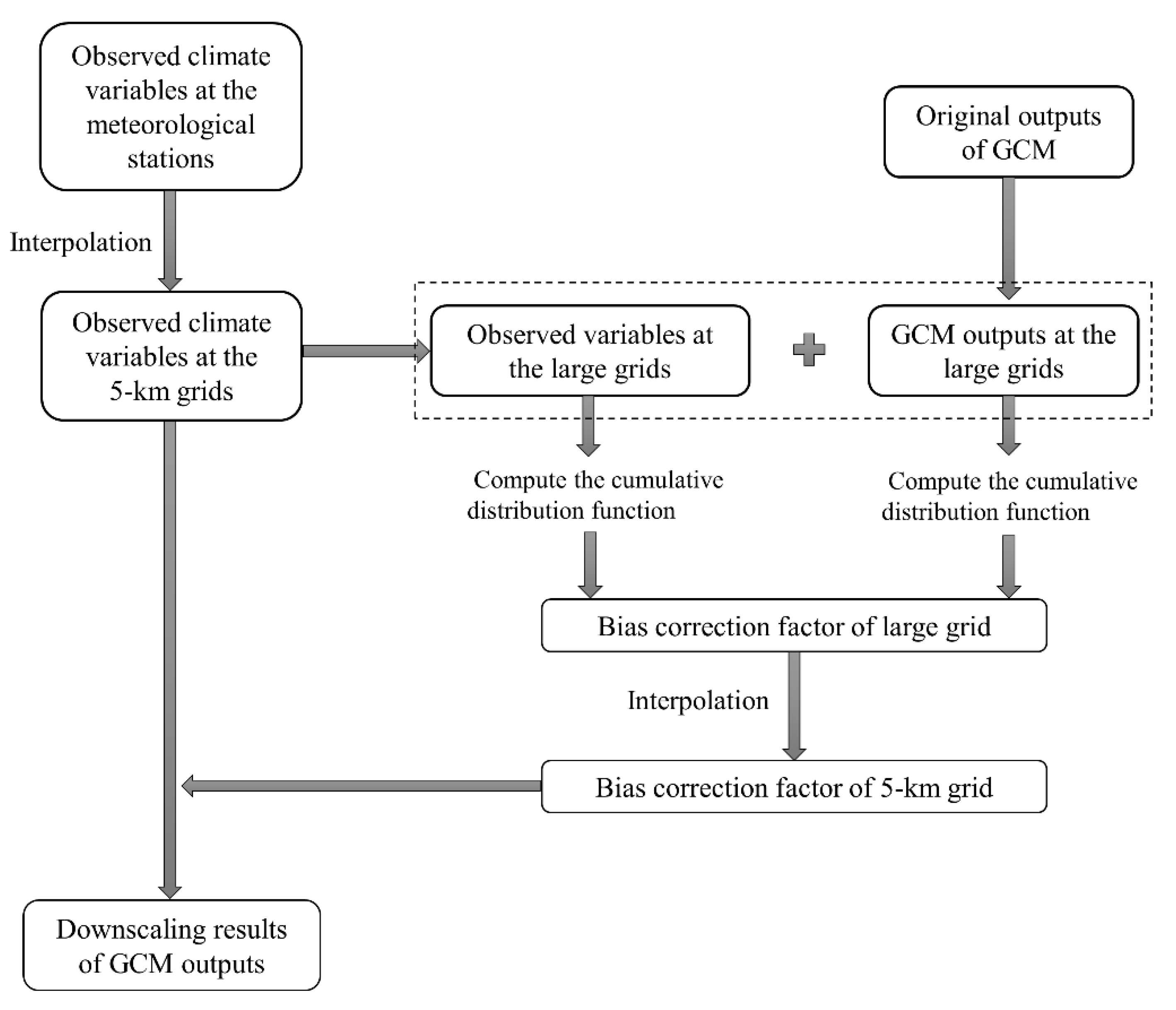
3.1. Bias Correction and Spatial Downscaling of GCM Output

In general, the climate variables simulated by the GCMs have certain biases compared with the observations. On the other hand, the spatial resolution of the output of the GCM is too coarse. Therefore, the outputs of GCMs cannot be directly applied to hydrological simulations at the catchment scale. Therefore, it is necessary to correct the biases of the variables provided by the GCM simulation and downscale them to the catchment scale. In this study, the BCSD (Bias Correction and Spatial Downscaling) method [30] was used to downscale the daily output of the GCMs to the grids of the hydrological model and correct the biases of them at the same time. In the BCSD method, the quantile mapping approach [30] was used to correct the biases of the GCM simulation based on the cumulative frequency curves of the measured climate elements in the baseline period. The cumulative frequency curves of the climate elements obtained after correction were consistent with the cumulative frequency curves of the observations [30]. The steps of the downscaling and bias correction of the GCM outputs (Figure 2) are summarized as follows:

(1)

The spatial resolution of the GCM outputs selected in this study is generally in the range of 0.75°–3°. Therefore, the daily outputs of the GCM were converted to the corresponding large grids (see Table 1).

(2)

The daily data observed at the meteorological stations were interpolated to a 5-km grid system using the inverse distance weighted method to obtain the observed climate variables at the 5-km grid scale. The observed climate variables at each large GCM grid were calculated based on the observed climate variables at 5-km grids within the large grid. Then, the quantile mapping method was used to correct the bias of the GCM outputs for the large grid. The values of the corrected variables of GCM at the large grid were compared with the observed variables to obtain the correction factors of the large grid.

(3)

The correction factors of the large grid were interpolated to the small grid of 5 km by the inverse distance weighted method to obtain the correction factors of each 5-km grid. Finally, based on the correction factor of each 5-km grid and the observed daily climate variables at the same grids, the downscaling results after bias correction at each 5-km grid were finally determined.

3.2. Brief Introduction of the Hydrological Model

The hydrological processes of the Amur River Basin were simulated by a distributed hydrological model, namely GBHM-HLJ [31], which was constructed for the Amur River Basin, and it was modified from the GBHM model (Geomorphology-Based Hydrological Model). The GBHM model has been successfully applied in many large watersheds, such as the Yangtze River Basin [32,33], the Yellow River Basin [34], the Mekong River Basin [35], the Chao Phraya River Basin [36] and the whole of Asia [37]. In this study, the model adopted a 5-km × 5-km grid system, and the study basin was discretized into 83,468 grid cells. The whole basin was divided into 209 subbasins, and within each subbasin, there were several flow intervals. The flow distances of the grid cells within the flow intervals were calculated using the GIS tools [38]. Within each grid, a “hillslope-valley” system was identified, and the hillslope was the basic unit for hydrological modeling [38,39]. On the hillslope, there were four layers in the vertical direction, including the vegetation layer, snow cover, the unsaturated zone and the groundwater aquifer. The movement of soil moisture in the unsaturated zone was described by the one-dimensional Richards equation. The excess infiltration runoff and saturation excess runoff were calculated on the hillslope unit, and the surface flows on the slope were calculated using the manning equation. The water balance equation and Darcy’s law were used to describe the relationship between the groundwater and the river. The river routing was calculated by the kinematic wave method. The Amur River Basin is located in the cold region of a high latitude. Therefore, the snowmelt and soil freeze–thaw cycle influence the runoff generation. In the model, the snowmelt was estimated by a temperature index method as follows [31,39]:

$${\mathrm{M}=\mathrm{f}}_{\mathrm{M}}{(\mathrm{T}-\mathrm{T}}_{\mathrm{b}})\mathsf{\Delta }\mathrm{t}$$

(1)

where M is the snowmelt runoff, f_M is degree–day factor (mm/°C.d). T is the air temperature (°C), T_b is the critical temperature of the snowmelt (°C) and ∆t is time step. The snowmelt factor f_M was obtained by the model calibrations.

A model describing the hydraulic conductivity of frozen soil was used to simulate the effect of a soil freezing–thawing cycle on the water movement. In this model, the hydraulic conductivity changed exponentially with the increase of the air temperature in the thawing period and the decrease of the air temperature in the freezing period:

$$\mathrm{K}=\{\begin{array}{c}{\mathrm{K}}_0\exp \left({\mathrm{k}}_{\mathrm{fz}}{(\mathrm{T}-\mathrm{T}}_1)\right),\mathrm{m}\le 6,\mathrm{T}\le {\mathrm{T}}_1\\ {\mathrm{K}}_0\exp \left({\mathrm{k}}_{\mathrm{fz}}{(\mathrm{T}+\mathrm{T}}_2)\right),\mathrm{m}\ge 7,\mathrm{T}\le {\mathrm{T}}_2\end{array}$$

(2)

where K is the hydraulic conductivity of frozen soil (mm/d), K₀ is the hydraulic conductivity of unfrozen soil with the same water content (mm/d), k_fz is the temperature factor of the frozen soil water conductivity (°C⁻¹), T is the air temperature, T₁ is the temperature hysteresis parameter of the frozen soil during the thawing period, m is the month, and the thawing period is usually before June, and T₂ is the temperature hysteresis parameter of the soil freezing development period, and the freezing development period is generally after July. The parameters k_fz, T₁ and T₂ were obtained by the model calibrations.

The details of the model are available in Gao et al., Cong et al., Yang et al. and Li et al. [31,33,34,38,39]. The Nash efficiency coefficient (NSE) and relative error (RE) were used to verify the applicability of the model in the study basin.

3.3. Statistical Methods for Analyzing the Changes in Runoff

In this study, the Pearson III-type curve was used for determining the flood peaks of different return periods. A Pearson III-type curve is an asymmetric curve with one finite end and another infinite end. The mean value, variation coefficient (C_v) and skewness coefficient (C_s) of the flood peaks were used to estimate the parameters of the Pearson III-type curve.

The Wilcoxon Signed-Rank test was used to examine the significance of the runoff changes. The Wilcoxon Signed-Rank test is widely used for examining the differences between paired data samples that come from two populations. The null hypothesis in this test was that there was no difference between the two samples. First, a new variable was calculated as follows [40]:

$$\mathrm{D}={\mathrm{x}}_1-{\mathrm{x}}_2$$

(3)

where x₁ and x₂ are the variables from the two different samples, respectively. By ranking D, the sum of the ranks of the positive differences ∑(+) and the negative differences ∑(−) is calculated. Next, the statistics were calculated as follows:

$$\mathrm{T}=\min [{\displaystyle \sum (+),{\displaystyle \sum (-)]}}$$

(4)

We rejected the null hypothesis when T was larger than the threshold value T_α corresponding to the significant level of α, which means that the difference between the two samples was significant. In this study, α was set to 0.05.

4. Results

4.1. Bias Correction of the GCM Output

Figure 3 displays a comparison between the basin-averaged value of the downscaled bias-corrected precipitation and air temperature of the GCM output and the observations in the baseline period. It can be seen from the figure that different GCMs generally have a certain ability to simulate the precipitation and air temperature in the Amur River Basin. For the air temperature estimation, the raw MRI-ESM2-0 model output had small errors, implying that the model performed better for simulating the monthly air temperature than the other models. The biases of all the GCMs were greatly reduced after correction. For the precipitation simulation, the original results of the four models all had non-negligible biases. In most cases, the models overestimated the monthly precipitation, and the underestimation of the observed precipitation was only detected in a few months in the summer for the BCC-CSM2-MR and EC-Earth3 models. The MRI-ESM2-0 and EC-Earth3 models simulated the precipitation well during the flood season, but they showed poor performances in estimating the precipitation during the non-flooding season. The precipitation simulated by the MIROC-ES2L model evidently overestimated the observations throughout the year, which may be related to its low spatial resolution. After the downscaling and bias correction using the BCSD method, the results of each GCM were quite close to the observations. This indicates that the BCSD method can effectively correct the biases of the outputs of the GCMs while downscaling.

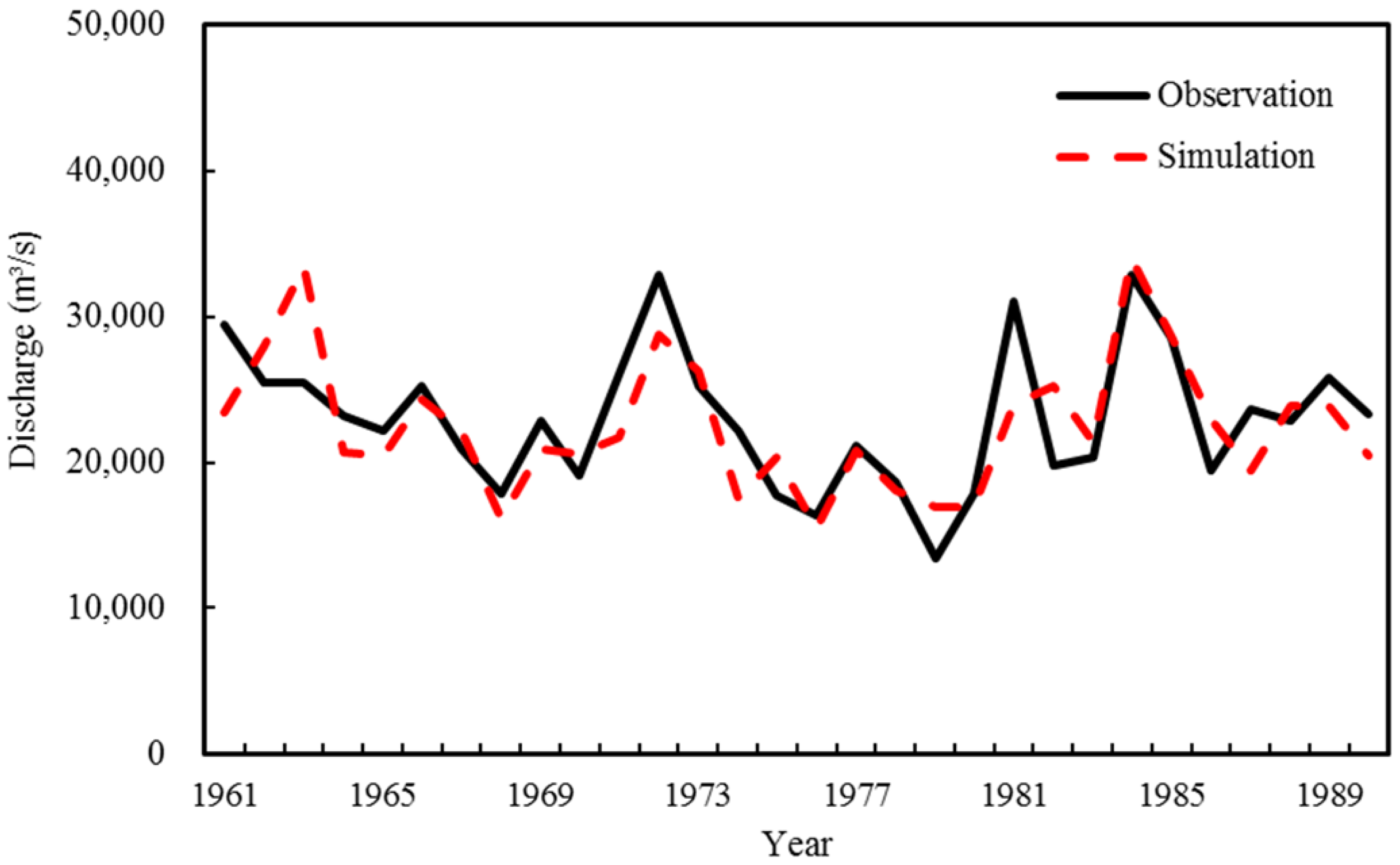
4.2. Validation of the Hydrological Model

In this study, the applicability of GBHM-HLJ in the Amur River Basin was validated by comparing the simulated river discharges and observations at the hydrological stations located on the main channel and major tributaries (

Table 2. Performance of GBHM-HLJ for the daily river discharge simulation at the main hydrological stations in the Amur River Basin for the calibration and validation periods.

Station	Calibration Period			Validation Period
	Period	RE	NSE	Period	RE	NSE
Kumara	1956–1959	−13.7%	0.81	1961–1965	−7.6%	0.80
Malinovka	1980–1985	7.2%	0.80	1986–1990	−8.7%	0.73
Harbin	1981–1985	2.1%	0.82	1986–1990	8.3%	0.83
Hoare	1981–1985	−1.8%	0.82	1986–1989	−11.1%	0.72
Khabarovsk	1981–1985	4.9%	0.90	1986–1990	−2.4%	0.89
Xiaoshazangka	1949–1953	9.1%	0.87	1954–1958	−6.7%	0.84

and Figure 1). The river roughness coefficient (n_c), slope shape coefficient (f_ss), the degree–day factor f_M and the parameters of the frozen soil hydraulic conductivity k_fz, T1 and T2, were calibrated. The other parameters were obtained from the measured or reference data. Figure 4 compares the simulated daily river discharge and observations at the Khabarovsk, Kumara and Xiaoshazangka Stations. The simulated discharges agreed well with the observations. Table 2 shows the assessment of the model performance at the main hydrological stations during the calibration period and the validation period. The NSE was commonly above 0.80, and the RE was less than 10%. The NSE and RE at Khabarovsk Station located at the lower reach of the main stream were 0.90 and 4.9% in the calibration period, and the NSE and RE were 0.89 and −2.4% in the validation period. These results indicate that the model exhibited good performance in simulating the daily river discharge in the Amur River Basin.

Figure 5 illustrates the variations of the model-simulated daily river discharge at Khabarovsk Station in the period from 1960 to 1990. The RE and NSE for this long sequence simulation were 0.8% and 0.89, respectively. Although the model simulation showed some deviations at the receding stage and the spring snowmelt period, the fluctuations of the observed daily discharges and the interannual variations of the flood peaks were well-captured. The simulated and observed annual maximum daily discharges at Khabarovsk Station are shown in Figure 6. It can be seen from the figure that the model simulations were in good agreement with the observations. These results showed that the GBHM-HLJ model had acceptable skills in simulating long-term changes in the river discharge and floods of the Amur River Basin.

4.3. Precipitation and Air Temperature Changes in the Future Period

Table 3. Change rates in the basin-averaged precipitation in the future period compared with that in the baseline period (%).

Scenario		BCC-CSM2-MR	MRI-ESM2-0	EC-Earth3	MIROC-ES2L	Ensemble Mean
SSP2-4.5	Spring	20.9	23.5	33.7	13.6	22.9
	Summer	8.8	16.5	11.8	6.9	11.0
	Autumn	9.6	16.3	22.8	12.7	15.4
	Winter	30.4	38.8	33.5	28.8	32.9
	August	8.5	13.6	9.6	9.0	10.2
	Annual	11.8	18.5	18.3	10.0	14.6
SSP5-8.5	Spring	18.7	26.0	28.5	19.0	23.0
	Summer	7.5	21.1	13.2	10.4	13.0
	Autumn	5.3	15.5	15.1	13.1	12.3
	Winter	29.6	40.6	38.5	13.0	30.4
	August	5.1	18.9	9.1	5.9	9.8
	Annual	9.7	21.5	17.0	12.4	15.2

and

Table 4. Changes in the basin-averaged air temperatures in the future period compared with that in the baseline period (°C).

Scenario		BCC-CSM2-MR	MRI-ESM2-0	EC-Earth3	MIROC-ES2L	Ensemble Mean
SSP2-4.5	Spring	1.98	2.10	3.45	2.83	2.59
	Summer	2.38	2.42	3.32	2.58	2.68
	Autumn	3.19	3.27	3.79	2.64	3.22
	Winter	3.34	2.58	3.03	2.69	2.91
	Annual	2.72	2.59	3.40	2.69	2.84
SSP5-8.5	Spring	3.61	2.67	3.73	3.16	3.30
	Summer	3.98	3.06	3.77	2.67	3.37
	Autumn	5.03	3.97	4.96	3.65	4.40
	Winter	5.14	3.05	4.08	4.49	4.19
	Annual	4.44	3.19	4.14	3.49	3.82

show the changes in the basin-averaged precipitation and air temperature in the Amur River Basin during the future period compared with the baseline period based on the downscaled and bias-corrected GCM outputs. In general, all the GCMs suggested an increase in the seasonal and annual precipitation in the future period. Under the SSP2-4.5 scenario, compared with the baseline period, the MRI-ESM2-0 and EC-Earth3 models suggested about an 18% increase in the annual precipitation, and the change rate estimated by the other two models was about 11%. The ensemble mean of the four models projected the annual precipitation increases by 14.6% under the SSP2-4.5 scenario. Under the SSP5-8.5 scenario, the MRI-ESM2-0 and MIROC-ES2L models projected larger increases in the annual precipitation than that under the SSP2-4.5 scenario, while the changes in the annual precipitation projected by the BCC-CSM2-MR and EC-Earth3 models were slightly lower than that under the SSP2-4.5 scenario. However, the models generally projected a larger increase in the summer precipitation under the SSP5-8.5 scenario than that under the SSP2-4.5 scenario, except for the BCC-CSM2-MR model. The ensemble mean of the four models projected an increase by 15.2% in the annual precipitation under the SSP5-8.5 scenario. In general, under these two scenarios, the increased rates of precipitation in the spring and winter were larger than those in the summer and autumn due to their low absolute values. Figure 7a,b shows the spatial distributions of the annual precipitation changes projected by the ensemble mean of the four GCMs in the two future climate scenarios. It can be seen from the figure that the annual precipitation exhibited a remarkable increase in the northern and northeastern parts of the basin, while the southeastern part of the basin showed the lowest changes.

In the future period, the results of all the four GCMs show that the air temperature in the Amur River Basin will significantly increase compared with the baseline period (Table 4). Under the SSP2-4.5 scenario, the ensemble mean of the four models projected an increase of 2.84 °C in the basin-averaged annual air temperature compared to that in the baseline period. Except for the MIROC-ES2L model, the other models suggested higher temperature increases in the autumn than in the spring. Under the SSP5-8.5 scenario, the increase in the basin-averaged annual air temperature in the Amur River Basin projected by the ensembles mean of the four models was 3.82 °C higher than that in the baseline period. These results indicate that the air temperature in the study area will have a larger increase under the SSP5-8.5 scenario than under the SSP2-4.5 scenario. From the perspective of spatial distribution, compared with the baseline period, the increase in the annual air temperature in the northern part was larger than that in the southern part (Figure 7c,d).

Figure S1 shows the interannual variations in the basin-averaged annual precipitation and air temperature in the baseline period and the two future scenarios. Generally, most GCMs showed larger variances of the precipitation and air temperature in the future period than that in the baseline period, and the variances under the SSP5-8.5 scenario were all greater than those under the SSP2-4.5 scenario. These results indicate that the future climate changes will increase the interannual variabilities of the precipitation and air temperature in the study basin, and the increases in the variabilities will tend to be more evident in the high-emissions scenario. The increasing trend in the air temperature under the SSP5-8.5 scenario was also greater than that in the baseline period and the SSP2-4.5 scenario, which also implies that the annual air temperature will tend to increase more significantly under the SSP5-8.5 scenario.

4.4. Changes in Runoff in the Future Period

Forced by the downscaled and bias-corrected results of the GCM outputs, we simulated the hydrological processes of the study basin in the baseline period and the future period using the GBHM-HLJ model. The runoff changes between the baseline period and the future period were analyzed.

Table 5. Change rates in the runoffs at Khabarovsk Station in the future period compared with those in the baseline period (%).

Scenario		Spring	Summer	Autumn	Winter	Flood Season (May-Sep)	Annual
SSP2-4.5	BCC-CSM2-MR	16.0 *	6.8 *	7.2 *	14.7 *	7.6 *	9.2 *
	MRI-ESM2-0	54.7 *	38.4 *	31.3 *	20.8 *	40.6 *	36.9 *
	EC-Earth3	54.3 *	18.3 *	23.4 *	22.4 *	25.0 *	25.8 *
	MIROC-ES2L	30.0 *	8.0 *	23.5 *	16.8 *	15.6 *	18.0 *
	Ensemble mean	37.0 *	18.0 *	21.7 *	19.1 *	22.1 *	22.5 *
SSP5-8.5	BCC-CSM2-MR	−0.9 *	−6.6 *	−7.0 *	12.4 *	−7.8 *	−4.2 *
	MRI-ESM2-0	54.7 *	45.7 *	43.1 *	29.3 *	47.8 *	44.8 *
	EC-Earth3	37.3 *	13.7 *	18.3 *	25.9 *	16.6 *	19.8 *
	MIROC-ES2L	22.2 *	9.3 *	18.7 *	25.9 *	12.6 *	16.2 *
	Ensemble mean	26.6 *	15.7 *	18.7 *	23.7 *	17.2 *	19.2 *

Note: The numbers marked with * mean that the changes were significant at the 95% confidence level (α = 0.05).

shows the degree of the annual and seasonal runoff changes at Khabarovsk Station relative to the baseline period under the SSP2-4.5 and SSP5-8.5 scenarios. In general, all four GCMs projected that the runoff will increase under the SSP2-4.5 scenario. However, the rates of change in the runoffs varied among the different models. The runoff increase estimated by BCC-CSM2-MR was lower than that of the other three models. For Khabarovsk Station, the multiyear average of the annual runoff will increase by 9.2–36.9% under the SSP2-4.5 scenario compared with that in the baseline period. Under the SSP5-8.5 scenario, the MIROC-ES2L model and the EC-Earth3 model projected lower degrees of increases in the runoffs than that under the SSP2-4.5 scenario. Moreover, the BCC-CSM2-MR model projected a decrease by 4.2% in the annual runoff under the SSP5-8.5 scenario compared with the baseline period. These results are because that the actual evaporations projected by these three GCMs had larger increases under the SSP5-8.5 scenario than that under the SSP2-4.5 scenario (Figure 8) due to the more significant warming. The increases in the runoffs at Khabarovsk Station projected by the ensemble mean of the four models were 22.5% and 19.2% under the SSP2-4.5 and SSP5-8.5 scenarios, respectively (Table 5). These results implied that the increase in the runoff under the SSP5-8.5 scenario will tend to be lower than under the SSP2-4.5 scenario. In the future period, the change rate in the runoff during the flood season was close to that of the annual runoff. Generally, the rates of increases in the runoffs during the spring and autumn were greater than that in the summer. On a monthly scale, the increases in the runoffs at Khabarovsk Station projected by different GCMs showed similar patterns, as shown in Figure 9. The runoffs increased significantly in August and September, with the lowest changes in June.

In addition, the runoff changes at the major stations located on the tributaries were also analyzed, and the results are displayed in

Table 6. Change rate of the annual runoffs at hydrological stations located on the tributaries in the future period compared with those in the baseline period (%).

Station		BCC-CSM2-MR	MRI-ESM2-0	EC-Earth3	MIROC-ES2L	Ensemble Mean
Xiaoshazangka	SSP2-4.5	5.1 *	26.2 *	8.1 *	19.1 *	14.6 *
	SSP5-8.5	−5.4	36.0 *	16.9 *	10.9 *	14.6 *
Harbin	SSP2-4.5	13.2 *	32.4 *	32.5 *	40.2 *	29.6 *
	SSP5-8.5	2.8 *	45.2 *	41.9 *	26.7 *	30.1 *
Malinovka	SSP2-4.5	12.7 *	37.5 *	22.3 *	21.1 *	23.5 *
	SSP5-8.5	−6.2	43.3 *	11.6 *	17.2 *	16.6 *
Kumara	SSP2-4.5	10.8 *	49.9 *	31.7 *	30.5 *	30.7 *
	SSP5-8.5	−7.1 *	56.9 *	36.8 *	52.8 *	34.9 *
Hoare	SSP2-4.5	1.5 *	36.9 *	23.3 *	−34.8 *	6.7 *
	SSP5-8.5	−7.8	28.2 *	7.2 *	−15.5 *	3.0 *

Note: The numbers marked with * mean that the changes were significant at the 95% confidence level (α = 0.05).

. In general, the annual runoffs in most of tributaries will increase in the future period. Except for BCC-CSM2-MR, the degree of runoff increases projected by the GCMs were basically in the range of 8–50%, and a few of them exceeded 50%. The changes in the runoff at Hoare Station at the Hoare River were quite limited, and the changes were relatively large at Harbin Station and Kumara Station with the increase in the annual runoff close to or exceeding 30%. On a monthly scale, the changes in the runoffs in the future period at the major stations located on the tributaries showed similar patterns as Khabarovsk Station, and one example is shown in Figure S2 in the Supplementary Materials.

Figure 7e,f shows the spatial variations in the changes in the runoff depths in the study basin in the future period compared with the baseline period. The spatial patterns of runoff changes were generally consistent with that of the precipitation. From the perspective of comparisons of the two scenarios, the spatial distributions of the runoff changes showed evident differences. The Upper Amur River Basin showed larger increases in the runoff under the SSP5-8.5 scenario than that under the SSP2-4.5 scenario, and the opposite was found in the Lower Amur River Basin.

4.5. Changes in Flood in the Future Period

Figure 10 and

Table 7. The multiyear average values of annual maximum daily discharge (m³/s) at Khabarovsk Station and its changes (%) in the future period compared with those in the baseline period.

	BCC-CSM2-MR	MRI-ESM2-0	EC-Earth3	MIROC-ES2L
1961–2010	18,175	18,799	19,154	19,013
2021–2070 (SSP2-4.5)	20,290	26,833	24,471	22,461
2021–2070 (SSP5-8.5)	18,266	29,643	22,799	21,418
Change (%) (SSP2-4.5)	11.6	42.7 *	27.8 *	18.1 *
Change (%) (SSP5-8.5)	5.0	57.7 *	19.0 *	12.6 *

Note: The numbers marked with * mean that the changes were significant at the 95% confidence level (α = 0.05).

show the changes in the annual maximum daily discharges at the main hydrological stations in the future period and the baseline period. For Khabarovsk Station, the annual maximum daily discharges increased in the future period compared to the baseline period, particularly for the maximum value of the annual maximum daily discharge. The mean value of the annual maximum daily discharge was significantly greater than that in the baseline period, with the exception of the projections by the BCC-CSM2-MR model. The MRI-ESM2-0 model projected the largest changes among the four GCMs under both the SSP2-4.5 and SSP5-8.5 scenarios. The changes projected by the GCMs under the SSP5-8.5 scenario were close to those under the SSP2-4.5 scenario, with the exception of the MRI-ESM2-0 model (Figure 10a). The degrees of the increases of the annual maximum daily river discharges at Khabarovsk Station projected by the ensemble mean of the four GCMs were 25.6% and 24.1% under the SSP2-4.5 and SSP5-8.5 scenarios, respectively. The changes in the annual maximum daily discharges in the future period at the other hydrological stations were generally similar to that at Khabarovsk Station (Figure 10). The BCC-CSM2-MR model commonly projected slight changes, and the other three models projected relative larger increases. These results suggested that the flood peak will increase in the future in the main stream and most tributaries of the Amur River.

The changes in the annual maximum 15-day flood volume are displayed in Figure 11. In general, increases in the annual maximum 15-day flood volumes were also commonly found at the hydrological stations located on the main channel and major tributaries. The tendencies of the annual maximum 15-day flood volume projected by the four GCMs in the future period were similar to the changes in the annual maximum daily discharges. The results projected by the MRI-ESM2-0 model generally showed the largest increases in the annual maximum 15-day flood volume, while the BCC-CSM2-MR model showed relatively limited changes.

Table 8. Change rates of the average and maximum values of the annual maximum 15-day flood volumes at Khabarovsk Station in the future period compared with those in the baseline period (%).

	Scenario	BCC-CSM2-MR	MRI-ESM2-0	EC-Earth3	MIROC-ES2L
Average	SSP2-4.5	11.1	41.9 *	27.9 *	18.7 *
	SSP5-8.5	0.3	55.6 *	20.3 *	12.5 *
Maximum	SSP2-4.5	65.4	16.6	32.5	13.5
	SSP5-8.5	62.7	32.7	22.6	7.6

Note: The numbers marked with * mean that the changes were significant at the 95% confidence level (α = 0.05).

shows the degree of change in the annual maximum 15-day flood volumes during the two future scenarios compared to the baseline period at Khabarovsk Station. The average rate of change projected by the BCC-CSM2-MR model was not significant; however, the change rate of the maximum value projected by the BCC-CSM2-MR model was the largest among the four GCMs.

The flood peaks of the return periods of 20 years and 50 years at Khabarovsk Station were estimated based on the Pearson III-type curve obtained by the simulated river discharges in the baseline period.

Table 9. The number of occurrences for the flood peaks of the 20-year and 50-year return periods at Khabarovsk Station in the baseline period and the future period.

Return Period	Period	BCC-CSM2-MR	MRI-ESM2-0	EC-Earth3	MIROC-ES2L
20 years	Baseline period	3	3	2	2
	SSP2-4.5	8	17	10	8
	SSP5-8.5	5	21	9	6
50 years	Baseline period	0	2	1	1
	SSP2-4.5	3	11	5	4
	SSP5-8.5	2	16	5	3

shows that all the four GCMs suggested that the frequency of flooding of both the 20-year and 50-year return periods will increase in the future, particularly for the MRI-ESM2-0 model, which showed the most evident increases. These results suggest that the frequency of floods in the Amur River Basin will tend to increase in the future. With the exception of the MRI-ESM2-0 model, the frequencies of floods projected by the GCMs under the SSP5-8.5 scenario were close to or lower than that under the SSP2-4.5 scenario, which was probably related to the higher temperature rising and larger evaporation under the SSP5-8.5 scenario, as mentioned in Section 4.4.

Figure 12 shows the flow duration curves at Khabarovsk Station under the future climate scenarios and the baseline period. The GCMs under the future climate scenarios generally projected increases of the high flows, but there were differences among the models. The GCMs projected significant increases in the amplitude and frequency of the high flows, except for the BCC-CSM2-MR model, which did not show increases in the high flows under the SSP5-8.5 scenario. The MRI-ESM2-0 model had the largest increase in high flows among the four GCMs at Khabarovsk Station. Figure S3 shows the flow duration curves of Xiaoshazangka Station at the Zeya River. The GCMs generally projected increases in the magnitude and frequency of the high flows in the future period, except for the BCC-CSM2-MR model, which projected decreases in the high flows under the SSP5-8.5 scenario. Similar results were also found at other stations located along the tributaries—for example, Malinovka Station and Kumara Station, shown in Figures S4 and S5. These results suggest that the frequency and magnitude of floods in the Amur River Basin will tend to increase in the future period.

4.6. Changes in Low Flows in the Future Period

In addition to floods, the changes in the low flows were also analyzed in this study. Figure 13 displays the changes in the annual minimum 7-day river discharges of the main channel and major tributaries in the future period. The GCMs generally suggested that the annual minimum 7-day river discharges in the future period were larger than that in the baseline period. The increases in the annual minimum 7-day river discharges under the SSP5-8.5 scenario were larger than those under the SSP2-4.5 scenario, with the exception of the EC-Earth3 model. Similar results were also found for the annual minimum 30-day river discharges, which are shown in Table S1 in the Supplementary Materials. At Khabarovsk Station, the annual minimum 30-day river discharges will significantly increase in the future period compared with the baseline period (Table S1). These results imply that the risk of hydrological drought will tend to be reduced in the future period.

5. Discussion

5.1. Impact of Future Climate Changes on Runoff

In this study, all the GCM project significant increases in the air temperature and precipitation in the future period, which suggest that the Amur River Basin will become wetter and warmer. These results are consistent with the findings of Yang et al. [11], which also projected significant increases in the air temperature and precipitation in this basin. Our results suggest that the runoffs in the upper and lower reaches of the Amur River will significantly increase in the future. The increases in the runoffs will provide more water resources and hydropower potential in the future; however, they will also increase the risk of floods in the Amur River Basin. The increases in precipitation projected by the ensemble mean of the GCMs under the SSP5-8.5 scenario were slightly larger than those under the SSP2-4.5 scenario. However, the increases in the runoffs projected by the ensemble mean of the GCMs under the SSP5-8.5 scenario were slightly lower than those under the SSP2-4.5 scenario due to larger increases in the actual evaporation. These results imply that the increases in evaporation resulting from the significant warming in the high-emission scenario will have a negative effect on the runoffs and may offset the positive effect of precipitation increase. The results of this study suggested that the low flows in the study basin will tend to increase in the future period, which may reduce the risk of hydrological drought. Considering the complex spatial and temporal characteristics of drought, more detailed studies by analyzing the relationships among the changes in the runoff, soil moisture and precipitation for better understanding the alterations of drought in future climate conditions are required in the future.

5.2. Uncertainties and Limitations

The uncertainties in projecting the future runoff changes were mainly induced by three sources: the GCM output, downscaling method and the hydrological model. Due to the coarse resolution of the GCM data, downscaling and bias correction of the GCMs are necessary. There are two types of downscaling methods, namely statistical downscaling and dynamic downscaling [41]. Dynamic downscaling requires a long time and large efforts for computations. Therefore, it is difficult to be applied for simulations forced by multi-GCMs [42]. Thus, the statistical downscaling method was used in this study due to its great efficiency. Previous studies have concluded that the uncertainties of the GCMs were greater than those of downscaling methods [43]. This is because the information on atmosphere systems that is available for climate studies and simulations is insufficient, and describing the complex nonlinear natural climate changes is still challenging in GCMs [44]. The most widely used methods in statistical downscaling are delta and quantile mapping [45]. The quantile mapping method was used in this study. However, quantile mapping may worsen trends in climates in some cases [46]. The BCSD assumes that the curves of the air temperature and precipitation frequency distributions are stationary over time. This assumption may not be valid for future climates [47]. At the same time, the BCSD model is based on the CDF function, which may have a certain influence on the timing of the GCM output.

Although uncertainties in the vegetation or soil parameters in such a large basin may also influence the accuracy of the runoff changes simulated by the hydrological model, the results of the validation for the hydrological model suggest that the GBHM-HLJ model forced by observed atmosphere forcings has high skills in simulating the hydrological processes and stream flows in the study basin. This implies that the uncertainties from the hydrological model are limited compared with those of the GCM and downscaling methods. Large differences in the magnitude of changes in runoffs projected by different GCMs were found in our studies. This result implies that the major uncertainties of the runoff projections in this study were from the GCMs. The changes in the annual runoffs and the flow duration curves had larger variations among the GCMs under the SSP5-8.5 scenario than that under the SSP2-4.5 scenario. This finding suggests that the uncertainties in the GCM projections of the runoffs were larger in the high-emission scenario than under the median-emission scenario. The GCMs selected in this study were based on the evaluations of their accuracies in previous studies, and the trends in precipitation and air temperature in the future period compared with the baseline period obtained by the four GCMs in this study were generally consistent with the pervious study of Yang et al. [11]. This increases the confidence in using these GCMs to analyze the changes in the runoffs in the future period. Comprehensively evaluating the uncertainties of all the GCMs in CMIP6 is a great challenge and will be one of our future works. In addition, the GBHM-HLJ model took the snowmelt and the freeze–thaw processes into consideration in the hydrological simulations in the study basin. However, this cryosphere module used in the GBHM-HLJ model was relatively simplified. Improving the accuracy in describing the cryosphere hydrological processes in the hydrological model will be another future work.

6. Conclusions

A distributed hydrological model, GBHM-HLJ, was calibrated and validated in the Amur River Basin. Based on the bias-corrected and spatial downscaling results of the outputs from four GCMs provided by the CMIP6, the hydrological processes of the Amur River Basin in the baseline period (1961–2010) and the future period (2021–2070) were simulated using the GBHM-HLJ model. The spatial and temporal variations in the impacts of future climate changes on the runoffs under the SSP2-4.5 and SSP5-8.5 scenarios were evaluated. The conclusions were as follows:

(1)

The validation of the GBHM-HLJ model shows that the model has acceptable skill in simulating the daily river flow in the Amur River Basin. It can provide high accuracy in simulating the long-term changes in the runoffs and floods.

(2)

Compared with the baseline period, the magnitude and variability of the precipitation and air temperature will evidently increase in the future period. The results of the ensemble mean of the four GCMs suggest that the basin-averaged annual precipitation will increase by 14.6% and 15.2% under the SSP2-4.5 and SSP5-8.5 scenarios, respectively. The basin-averaged annual air temperatures projected by the ensemble mean of the four GCMs will rise by 2.84 °C under the SSP2-4.5 scenario and 3.82 °C under the SSP5-8.5 scenario.

(3)

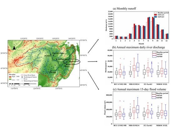
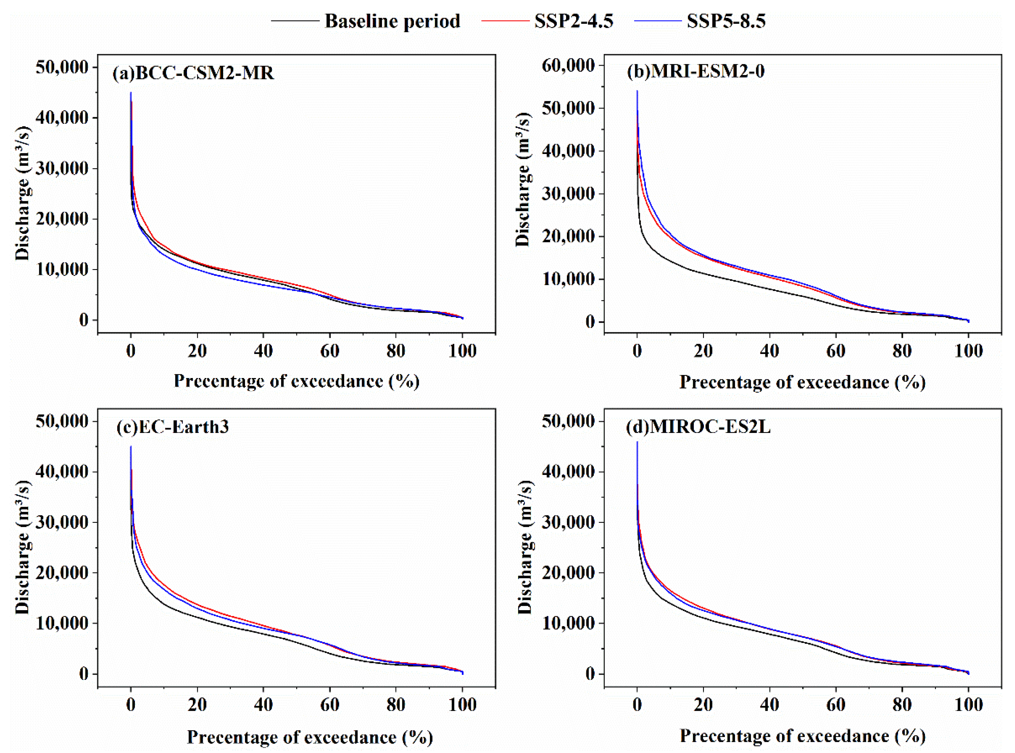
The results suggest that the river discharges of the main channel and the major tributaries will tend to increase in the future period compared with the baseline period, particularly in August and September. The results of the ensemble mean of the four GCMs suggest that the basin-averaged annual runoff will increase by 22.5% and 19.2% at Khabarovsk Station under the SSP2-4.5 and SSP5-8.5 scenarios, respectively. The annual maximum daily river discharge, annual maximum 15-day flood volume and the frequency of flooding will also tend to increase in the future period.

(4)

Although increasing trends in the precipitation and runoffs were commonly found in the future period compared with the baseline period, large differences among the different GCMs and scenarios still existed, particularly for the runoff. The BCC-CSM2-MR model projected a decrease in the runoff under the SSP5-8.5 scenario, and it suggested a lower magnitude of increase in the runoff and high flows than the other GCMs under the SSP2-4.5 scenario. Due to the larger increase in evaporation, the runoff increase under the SSP5-8.5 scenario was lower than that under the SSP2-4.5 scenario.

The findings of this study suggest that the streamflow in the Amur River Basin will tend to increase in the near future. This will benefit water resource developments. However, the significant increase in the high flows also highlights that the risk of flooding may also increase in the future. Therefore, water resource managers should take effective adaptions to mitigate this increasing trend of flood risk. This work is a first step toward assessing the responses of runoffs in the Amur River Basin to future climate changes. Further analyses of the cryosphere changes in the future climate conditions and a more comprehensive evaluation of the uncertainties in runoff projection will be addressed in future studies.

References

1. IPCC. Summary for Policymakers. In Climate Change 2021: The Physical Science Basis. Contribution of Working Group I to the Sixth Assessment Report of the Intergovernmental Panel on Climate Change; Masson-Delmotte, V., Zhai, P., Pirani, A., Connors, S.L., Péan, C., Berger, S., Caud, N., Chen, Y., Goldfarb, L., Gomis, M.I., et al., Eds.; Cambridge University Press: Cambridge, UK, 2021; in press. [Google Scholar]
2. Oo, H.T.; Zin, W.W.; Thin Kyi, C.C. Assessment of Future Climate Change Projections Using Multiple Global Climate Models. Civ. Eng. J. 2019, 5, 2152–2166. [Google Scholar] [CrossRef] [Green Version]
3. Zakizadeh, H.R.; Ahmadi, H.; Zehtabiyan, G.R.; Moeini, A.; Moghaddamnia, A. Impact of climate change on surface runoff: A case study of the Darabad River, northeast of Iran. J. Water Clim. Chang. 2021, 12, 82–100. [Google Scholar] [CrossRef]
4. Farsi, N.; Mahjouri, N. Evaluating the contribution of the climate change and human activities to runoff change under uncertainty. J. Hydrol. 2019, 574, 872–891. [Google Scholar] [CrossRef]
5. Shadmehri Toosi, A.; Doulabian, S.; Ghasemi Tousi, E.; Calbimonte, G.H.; Alaghmand, S. Large-scale flood hazard assessment under climate change: A case study. Ecol. Eng. 2020, 147, 105765. [Google Scholar] [CrossRef]
6. Muelchi, R.; Rössler, O.; Schwanbeck, J.; Weingartner, R.; Martius, O. River runoff in Switzerland in a changing climate—Runoff regime changes and their time of emergence. Hydrol. Earth Syst. Sci. 2021, 25, 3071–3086. [Google Scholar] [CrossRef]
7. Yu, L.; Xia, Z.; Li, J.; Cai, T. Climate change characteristics of Amur River. Water Sci. Eng. 2013, 131–144. [Google Scholar] [CrossRef]
8. Sun, W.; Fan, H. The Latest Change of Temperature in Songhua River Basin Under the Background of Global Warming. Soil Water Conserv. Res. 2018, 25, 97–104. (In Chinese) [Google Scholar]
9. Zhou, S.; Zhang, W.; Guo, Y. Impacts of Climate and Land-Use Changes on the Hydrological Processes in the Amur River Basin. Water 2019, 12, 76. [Google Scholar] [CrossRef] [Green Version]
10. Bolgov, M.V.; Trubetskova, M.D.; Filippova, I.A.; Kharlamov, M.A. Characteristics of extreme precipitation events within the Amur river basin in summer 2013. Geogr. Nat. Resour. 2017, 38, 139–146. [Google Scholar] [CrossRef]
11. Yang, X.; Zhou, B.; Xu, Y.; Han, Z. CMIP6 Evaluation and Projection of Temperature and Precipitation over China. Adv. Atmos. Sci. 2021, 38, 817–830. [Google Scholar] [CrossRef]
12. Shin, Y.; Jung, H. Assessing uncertainty in future climate change in Northeast Asia using multiple CMIP5 GCMs with four RCP scenarios. J. Environ. Impact Assess. 2015, 24, 205–216. [Google Scholar] [CrossRef] [Green Version]
13. Mauser, W.; Bach, H. PROMET—Large scale distributed hydrological modelling to study the impact of climate change on the water flows of mountain watersheds. J. Hydrol. 2009, 376, 362–377. [Google Scholar] [CrossRef]
14. Singh, V.P.; Woolhiser, D.A. Mathematical Modeling of Watershed Hydrology. J. Hydrol. Eng. 2002, 7, 270–292. [Google Scholar] [CrossRef] [Green Version]
15. Kiprotich, P.; Wei, X.; Zhang, Z.; Ngigi, T.; Qiu, F.; Wang, L. Assessing the Impact of Land Use and Climate Change on Surface Runoff Response Using Gridded Observations and SWAT+. Hydrology 2021, 8, 48. [Google Scholar] [CrossRef]
16. Prasch, M.; Marke, T.; Strasser, U.; Mauser, W. Large Scale Distributed Hydrological Modelling. In Applied Geoinformatics for Sustainable Integrated Land and Water Resources Management (ILWRM) in the Brahmaputra River Basin; Springer: New Delhi, India, 2015; pp. 37–43. [Google Scholar] [CrossRef]
17. Huang, Y.; Xiao, W.; Hou, B.; Zhou, Y.; Hou, G.; Yi, L.; Cui, H. Hydrological projections in the upper reaches of the Yangtze River Basin from 2020 to 2050. Sci. Rep. 2021, 11, 9720. [Google Scholar] [CrossRef]
18. Guimberteau, M.; Ciais, P.; Ducharne, A.; Boisier, J.P.; Dutra Aguiar, A.P.; Biemans, H.; De Deurwaerder, H.; Galbraith, D.; Kruijt, B.; Langerwisch, F.; et al. Impacts of future deforestation and climate change on the hydrology of the Amazon Basin: A multi-model analysis with a new set of land-cover change scenarios. Hydrol. Earth Syst. Sci. 2017, 21, 1455–1475. [Google Scholar] [CrossRef] [Green Version]
19. Zhang, L.; Yuan, F.; Wang, B.; Ren, L.; Zhao, C.; Shi, J.; Liu, Y.; Jiang, S.; Yang, X.; Chen, T.; et al. Quantifying uncertainty sources in extreme flow projections for three watersheds with different climate features in China. Atmos. Res. 2021, 249, 105331. [Google Scholar] [CrossRef]
20. Wang, Z.; Tian, Q.; Wan, L.; Yang, X. Runoff simulation in Harbin section of Songhua River basin based on SWAT model. Environ. Monit. Manag. Technol. 2015, 27, 10–14. (In Chinese) [Google Scholar]
21. Li, H.; Li, Y.; Liu, H.; Wang, X.; Wang, S.; Wang, A. Adaptability analysis of SIMHYD model in Songhua River basin. J. Jilin Univ. (Earth Sci. Ed.) 2017, 47, 1502–1510. (In Chinese) [Google Scholar]
22. Dai, C.; Wang, S.; Li, Z.; Zhang, Y.; Gao, Y.; Li, C. Study on the Water Potential of the Heilongjiang (Amur River) Basin; Heilongjiang Education Press: Harbin, China, 2014; Volume 11, pp. 35–38. (In Chinese) [Google Scholar]
23. Liu, S.; Zhang, L.; Cai, Y. Report on the Scientific Investigation of Large River Basins and Typical Lakes in Northern China and Its Adjacent Areas; Science Press: Beijing, China, 2017; pp. 36–44. (In Chinese) [Google Scholar]
24. Bazarova, V.B.; Mokhova, L.M.; Klimin, M.A.; Kopoteva, T.A. Vegetation development and correlation of Holocene events in the Amur River basin, NE Eurasia. Quat. Int. 2011, 237, 83–92. [Google Scholar] [CrossRef]
25. Yan, B.; Zhang, X.; Xia, Z.; Guo, M.; Liu, C.; Luo, Y. Analysis on the characteristics of precipitation change in Heilongjiang (Amur River) Basin. J. Yangtze River Sci. Res. Inst. 2019, 36, 14–17. [Google Scholar] [CrossRef]
26. Xiao, D.; Zhang, X. Preliminary analysis of hydrology and water resources characteristics in Heilongjiang (Amur River) Basin. J. China Hydrol. 1992, 5, 51–53. (In Chinese) [Google Scholar]
27. Wieder, W.R.; Boehnert, J.; Bonan, G.B.; Langseth, M. Regridded Harmonized World Soil Database, Version 1.2; Oak Ridge National Laboratory Distributed Active Archive Center (ORNL DAAC): Oak Ridge, TN, USA, 2014. [Google Scholar]
28. O’Neill, B.C.; Tebaldi, C.; van Vuuren, D.P.; Eyring, V.; Friedlingstein, P.; Hurtt, G.; Knutti, R.; Kriegler, E.; Lamarque, J.-F.; Lowe, J.; et al. The Scenario Model Intercomparison Project (ScenarioMIP) for CMIP6. Geosci. Model Dev. 2016, 9, 3461–3482. [Google Scholar] [CrossRef] [Green Version]
29. Jiang, D.; Hu, D.; Tian, Z.; Lang, X. Differences between CMIP6 and CMIP5 models in simulating climate over china and the east Asian monsoon. Adv. Atmos. Sci. 2020, 37, 1102–1118. [Google Scholar] [CrossRef]
30. Wood, A.W.; Leung, L.R.; Lettenmaier, V. Hydrologic Implications of Dynamical and Statistical Approaches to Downscaling Climate Model Outputs. Clim. Chang. 2004, 62, 189–216. [Google Scholar] [CrossRef]
31. Li, M.; Yang, D.; Hou, J.; Xiao, P.; Xing, G. A Distributed Hydrological Model of the Heilongjiang River (Amur River) Basin. J. Hydroelectr. Eng. 2021, 40, 65–75. (In Chinese) [Google Scholar]
32. Xu, J.; Yang, D.; Yi, Y.; Lei, Z.; Chen, J.; Yang, W. Spatial and temporal variation of runoff in the Yangtze River basin during the past 40 years. Quat. Int. 2008, 186, 32–42. [Google Scholar] [CrossRef]
33. Gao, B.; Li, J.; Wang, X. Analyzing Changes in the Flow Regime of the Yangtze River Using the Eco-Flow Metrics and IHA Metrics. Water 2018, 10, 1552. [Google Scholar] [CrossRef] [Green Version]
34. Cong, Z.; Yang, D.; Gao, B.; Yang, H.; Hu, H. Hydrological trend analysis in the Yellow River basin using a distributed hydrological model. Water Resour. Res. 2009, 45. [Google Scholar] [CrossRef]
35. Wang, W.; Lu, H.; Yang, D.; Khem, S.; Yang, J.; Gao, B. Modelling hydrologic processes in the Mekong River basin using a distributed model driven by satellite precipitation and rain gauge observations. PLoS ONE 2016, 11, e0152229. [Google Scholar] [CrossRef] [PubMed] [Green Version]
36. Yang, S.; Yang, D.; Chen, J.; Santisirisomboon, J.; Lu, W.; Zhao, B. A physical process and machine learning combined hydrological model for daily streamflow simulations of large watersheds with limited observation data. J. Hydrol. 2020, 590, 125206. [Google Scholar] [CrossRef]
37. Yang, D.; Musiake, K. A continental scale hydrological model using distributed approach and its application to Asia. Hydrol. Process. 2003, 17, 2855–2869. [Google Scholar] [CrossRef]
38. Yang, D.; Herath, S.; Musiake, K. Development of a geomorphology-based hydrological model for large catchments. Proc. Hydraul. Eng. 1998, 42, 169–174. [Google Scholar] [CrossRef] [Green Version]
39. Yang, D.; Herath, S.; Musiake, K. A hillslope-based hydrological model using catchment area and width functions. Hydrol. Sci. J. 2002, 47, 49–65. [Google Scholar] [CrossRef]
40. Ohyver, M.; Moniaga, J.V.; Sungkawa, I.; Subagyo, B.E.; Chandra, I.A. The Comparison Firebase Realtime Database and MySQL Database Performance using Wilcoxon Signed-Rank Test. Procedia Comput. Sci. 2019, 157, 396–405. [Google Scholar] [CrossRef]
41. Xue, Y.; Janjic, Z.; Dudhia, J.; Vasic, R.; De Sales, F. A review on regional dynamical downscaling in intraseasonal to seasonal simulation/prediction and major factors that affect downscaling ability. Atmos. Res. 2014, 147–148, 68–85. [Google Scholar] [CrossRef] [Green Version]
42. Wu, Q.; He, Z.; Nie, Q.S.; Gui, B. Evaluation of wind energy simulated by dynamical downscaling methods for Poyang Lake. Resour. Sci. 2012, 34, 2337–2346. (In Chinese) [Google Scholar]
43. Wilby, R.L.; Harris, I. A framework for assessing uncertainties in climate change impacts: Low-flow scenarios for the River Thames, UK. Water Resour. Res. 2006, 42. [Google Scholar] [CrossRef]
44. Qin, D. Climate and Environment Changes in China (Volume1): Climate and Environment Changes and Predition; Science Press: Beijing, China, 2005; pp. 45–47. (In Chinese) [Google Scholar]
45. Moghim, S.; Bras, R.L. Bias Correction of Climate Modeled Temperature and Precipitation Using Artificial Neural Networks. J. Hydrometeorol. 2017, 18, 1867–1884. [Google Scholar] [CrossRef]
46. Maurer, E.P.; Pierce, D.W. Bias correction can modify climate model simulated precipitation changes without adverse effect on the ensemble mean. Hydrol. Earth Syst. Sci. 2014, 18, 915–925. [Google Scholar] [CrossRef] [Green Version]
47. Hayhoe, K.; Wake, C.P.; Huntington, T.G.; Luo, L.; Schwartz, M.D.; Sheffield, J.; Wood, E.; Anderson, B.; Bradbury, J.; DeGaetano, A.; et al. Past and future changes in climate and hydrological indicators in the US Northeast. Clim. Dyn. 2006, 28, 381–407. [Google Scholar] [CrossRef]
Figure 1. Topography, river network, the meteorological gauge and hydrological stations in the Amur River Basin.
Atmosphere 12 01560 g001
Figure 2. Flowchart of the BCSD method used in this study.
Atmosphere 12 01560 g002
Figure 3. Monthly basin-averaged precipitation and air temperature of the GCMs before and after bias corrections and observations in the baseline period. (a) BCC-CSM2-MR (b) MRI-ESM2-0 (c) EC-Earth3 (d) MIROC-ES2L.
Atmosphere 12 01560 g003
Figure 4. Simulated daily river discharges by GBHM-HLJ and observations during the calibration and validation periods at: (a) Khabarovsk Station, (b) Kumara Station and (c) Xiaoshazangka Station.
Atmosphere 12 01560 g004
Figure 5. Long-term simulations of the daily river discharge at Khabarovsk Station using the GBHM-HLJ model from the observed atmosphere forcings and observed daily river discharges.
Atmosphere 12 01560 g005
Figure 6. Simulated and observed annual maximum daily discharges at Khabarovsk Station.
Atmosphere 12 01560 g006
Figure 7. Spatial variations of the changes in the annual precipitation, air temperatures and runoff depths under the future climate scenarios compared with the baseline period: (a,c,e) under the SSP2-4.5 scenario and (b,d,f) under the SSP5-8.5 scenario. (a,b) The same legend and (e,f) the same legend.
Atmosphere 12 01560 g007
Figure 8. Spatial variations in the annual actual evaporations in the baseline period and under the future climate scenarios. (a,d,g,j) In the baseline period, (b,e,h,k) under the SSP2-4.5 scenario and (c,f,i,l) under the SSP5-8.5 scenario.
Atmosphere 12 01560 g008
Figure 9. Model-simulated monthly runoffs at Khabarovsk Station in the baseline period and under the future climate scenarios. (a) BCC-CSM2-MR (b) MRI-ESM2-0 (c) EC-Earth3 (d) MIROC-ES2L.
Atmosphere 12 01560 g009
Figure 10. Box plot of the model-simulated annual maximum daily river discharges in the baseline period and under the future climate scenarios. (a) Khabarovsk (b) Xiaoshazangka (c) Kumara (d) Malinovka (e) Hoare.
Atmosphere 12 01560 g010
Figure 11. Box plot of the model-simulated annual maximum 15-day flood volumes in the baseline period and under the future climate scenarios. (a) Khabarovsk (b) Xiaoshazangka (c) Kumara (d) Malinovka (e) Hoare.
Atmosphere 12 01560 g011
Figure 12. Comparisons of the model-simulated flow duration curves of Khabarovsk Station in the baseline period and under the future climate scenarios. (a) BCC-CSM2-MR (b) MRI-ESM2-0 (c) EC-Earth3 (d) MIROC-ES2L.
Atmosphere 12 01560 g012
Figure 13. Box plot of the model-simulated annual minimum 7-day river discharges in the baseline period and under the future climate scenarios. (a) Khabarovsk (b) Xiaoshazangka (c) Kumara (d) Malinovka (e) Hoare.
Atmosphere 12 01560 g013