Isolated Effects of Indian Ocean Basin-Wide and El Niño–Southern Oscillation on Austral Winter Rainfall over South America

Abstract

Contrasting effects of the tropical Indian and Pacific Oceans on the atmospheric circulation and rainfall interannual variations over South America during southern winter are assessed considering the effects of the warm Indian Ocean basin-wide (IOBW) and El Niño (EN) events, and of the cold IOBW and La Niña events, which are represented by sea surface temperature-based indices. Analyses are undertaken using total and partial correlations. When the effects of the two warm events are isolated from each other, the contrasts between the associated rainfall anomalies in most of South America become accentuated. In particular, EN relates to anomalous wet conditions, and the warm IOBW event to opposite conditions in extensive areas of the 5° S–25° S band. These effects in the 5° S–15° S sector are due to the anomalous regional Hadley cells, with rising motions in this band for the EN and sinking motions for the warm IOBW event. Meanwhile, in subtropical South America, the opposite effects of the EN and warm IOBW seem to be due to the presence of anomalous anticyclone and cyclone and associated moisture transport, respectively. These opposite effects of the warm IOBW and EN events on the rainfall in part of central South America might explain the weak rainfall relation in this region to the El Niño–Southern Oscillation (ENSO). Our results emphasize the important role of the tropical Indian Ocean in the South American climate and environment during southern winter.

1. Introduction

The El Niño–Southern Oscillation (ENSO) is the primary source of interannual climate variability over much of South America, where it causes extreme climate conditions through changes in the regional atmospheric circulation, which in the tropics are regulated by anomalous Walker and local Hadley cells [1], and in the subtropics and extratropics by Rossby wave train teleconnection patterns [2,3]. The ENSO impact on the South American rainfall varies during the ENSO cycle and presents large spatiotemporal variability [4,5,6,7,8,9,10,11,12]. Considering the annual total precipitation, typical ENSO-related rainfall anomalies over South America feature a dipole-like pattern between its northern-northeastern and southeastern sectors with El Niño (EN) related droughts over equatorial South America [13]. Detailed studies reveal seasonal differences in these anomalies. The EN-related excessive rainfall in southeastern South America (SESA) occurs during the southern spring and summer of the EN years [4] and during autumn and winter of eastern Pacific (or canonical) EN years [14]. The rainfall anomalies in SESA are modulated by the EN-related Rossby wave train pattern [3], which intensifies the rainfall controlling factors in the region, such as the subtropical jet stream [9] and South American Low-Level Jet [1]. During the La Niña events, the anomalous circulation and rainfall patterns are reversed [5,13]. An extensive review of the ENSO impacts on South American rainfall, including the Indian Ocean teleconnection, can be found in Cai et al. [15].

The relative role of the Indian and Pacific Oceans on the South American rainfall variability was previously examined [16,17]. Drumond and Ambrizzi [16] found that anomalous warm waters in the subtropical Indian Ocean are linked to increased southern summer rainfall in subtropical South America via a Rossby wave train pattern. Taschetto and Ambrizzi [17] focused on the dominant sea surface temperature (SST) anomaly mode in the tropical Indian Ocean, which is called the Indian Ocean basin-wide (IOBW) mode. This mode illustrates ENSO-induced uniform warming or cooling in the tropical Indian Ocean [18], with EN generating a warm IOBW event and La Niña, a cold IOBW event [19], and has its largest variability during southern summer and autumn [20]. Considering that the warm IOBW and EN events co-exist, Taschetto and Ambrizzi [17] argued that the warm IOBW event strengthens the EN-related atmospheric circulation and rainfall anomalies over South America during southern autumn and contributes to the persistency of dryness in northeastern Brazil (NEB). Nevertheless, Kayano et al. [21] provided diagnostic evidence that the EN and warm IOBW have opposite effects in the austral summer rainfall in this region, with EN causing anomalous dryness.

Most studies on the rainfall variability over South America have overlooked the rainfall variations during the southern winter, mainly because this season overlaps the three driest months over much of South America [8]. However, a better knowledge of the factors that might modulate the southern winter rainfall over South America is important for climate and environmental monitoring and might support modeling studies. Thus, it is clear that further analyses on the southern winter rainfall variability in South America are needed. Since the IOBW and EN events co-occur, in the present analysis, we adopted the same diagnostic method used by Taschetto and Ambrizzi [17]. However here, we focused on the southern winter season, and instead of the Niño-3 SST index (SST anomalies mean in the 5° N–5° S; 150° W–90° W) used by Taschetto and Ambrizzi [17] to describe the ENSO variability, and the principal component (PC) time series of the first empirical orthogonal function (EOF) variability mode of the SST anomalies in the tropical Pacific was used. Thus, the relative role of the ENSO and IOBW events on the South American rainfall during southern winter is examined here using total and partial correlation analyses. The following section presents a brief description of the data and methodology. Section 3 presents the rainfall and anomaly patterns associated with the warm IOBW and EN. Discussions and Conclusions are drawn in Section 4.

2. Data and Methods

The data used consist of monthly averages of the zonal and meridional winds, specific humidity, vertical velocity in pressure coordinates at standard surface pressure levels taken from the National Centers for Environmental Prediction/National Center for Atmospheric Research (NCEP/NCAR) Reanalysis-I Project dataset provided by the NOAA/OAR/ESRL PSL, Boulder, CO, USA [22]. These data are on a 2.5° horizontal resolution grid and at eleven standard surface pressure levels from 1000 to 150 hPa. The streamfunction data were obtained from the NCEP/NCAR Reanalysis-I and are in a Gaussian grid of 192 by 94 points at sigma levels 0.8458 and 0.2101, which correspond approximately to 850 hPa and 200 hPa, respectively. Additionally, monthly precipitation data from the Global Precipitation Climatology Centre Full Data Reanalysis V.8 version [23] and monthly SST data from the extended reconstructed SST version V5 dataset [24] were also used. The precipitation and SST data are on rectangular grids, respectively, on 1° and 2° horizontal resolution. All data were obtained for the 1951–2016 period from the National Oceanic and Atmospheric Administration (NOAA) website at psl.noaa.gov/data/gridded/index.html, acessed on 21 October 2021.

The asymmetric streamfunction (PSI) data were used. The vertically integrated moisture flux components (1000–300 hPa) and their divergence were calculated using the equations in Peixoto and Oort [25] (their equation 12.5 pp. 274). This vector is referred to as VIMF and the vector wind at 850 hPa as WIND. Vertical velocities averaged in the 5° N–5° S band are used to represent the Walker cell and are referred to as WVEL. Vertical velocities averaged in the 62.5° W–57.5° W longitudinal band are used to represent a regional Hadley cell over the Tropical North Atlantic (TNA)/South American region and are referred to as HVEL. Additionally, 500 hPa vertical velocity (VVEL500) in pressure coordinates was also used.

The southern winter (June to August -JJA) precipitation in South America shows significant linear trends over the 1951–2016 period (Figure not shown). Because linear trends in the variables affect the results, the analysis here is based on detrended variables. So, before calculating JJA values, the linear trends in all variables over 1951–2016 were removed from the monthly data in each grid point using the least-squares method.

Since the present analysis is for the southern winter, the averaged data for these months were used. The winter standardized anomaly time series were based on winter means and standard deviations for the 1951–2016 base period. In order to isolate the interannual time scale fluctuations, the anomaly time series were subjected to a Morlet wavelet bandpass filter (2–7-year), which is defined with equation 29 in Torrence and Compo [26]. The Morlet wavelet is defined as a complex exponential modulated by a Gaussian, ${\psi }_0\left(n\right)={\pi }^{\frac{-1}{4}} e^{i{\omega }_o\eta }{e}^{\frac{-{\eta }^2}{2}}$, with $\eta =\frac{t}{s}$, where t is the time, s, the wavelet scale, and ${\omega }_0$, a non-dimensional frequency which is taken to be 6 to satisfy admissibility condition (Torrence and Compo 1998). For a discrete sequence $x_n$, the filtered series between scales $j_1$ and $j_2$ is given after Torrence and Compo [26]:

$$x_n^{\prime }=\frac{{\delta }_j{\delta }_t^{\frac{1}{2}}}{C_{\delta }{\psi }_0\left(0\right)}{\displaystyle \sum }_{j=j_1}^{j_2}\frac{R\left\{W_{n\left(s_j\right)}\right\}}{s_j^{\frac{1}{2}}}$$

(1)

where, $W_n\left(s\right)$ is the wavelet transform, $\delta$ is the delta function, $C_{\delta }$ is an empirically derived factor equal to 0.776 for the Morlet wavelet, ${\delta }_j$ and ${\delta }_t$ are the time steps.

The IOBW mode was identified by applying the EOF analysis on the winter filtered SST anomalies in the tropical Indian Ocean (26° N–26° S; 30° E–120° E) during the 1951–2016 period. The PC time series associated with the IOBW mode was used as the IOBW index. Similarly, the ENSO mode and its index were obtained from the EOF analysis of the filtered winter SST anomalies in the tropical Pacific Ocean (30° N–30° S; 110° E–70° W) during the 1951–2016 period. The PC time series corresponding to the ENSO mode was used as the ENSO index and called the tropical Pacific Ocean (TPO) index. The EOF analysis was based on the covariance matrix and the separation of the eigenvalues on North et al.’s [27] criterion. The eigenvectors were displayed as correlation patterns, whose statistical significance was tested using the Student’s t-test for 66 degrees of freedom [28]. Absolute correlations exceeding 0.25 are significant at a 95% confidence level. The IOBW and TPO indices are such that their positive values correspond to the warm IOBW and EN events, respectively. Figure 1 illustrates South America and the areas in the tropical Indian and Pacific Oceans used here.

The relationships between the IOBW and TPO indices and the atmospheric circulation and rainfall anomalies were obtained from the total and partial correlations for the 1951–2016 period. For conciseness, the total correlation between a given oceanic index ‘IDX’ and a given variable ‘Y’ is referred to as ‘[IDX × Y]’; the partial correlation of the oceanic index ‘IDX1′ and a given variable ‘Y,’ while excluding the influence of the oceanic index ‘IDX2′ is referred to as ‘[IDX1 × Y minus IDX2]’, which means correlation after removing the influence of ‘IDX2′ on ‘IDX1′ and ‘Y’ using linear regression. Simultaneous correlations imply that the two warm events may co-exist during the southern winter. Because the ENSO is seasonally phase-locked, in general, the EN events during the southern winter are in their onset or demise phases. The correlation significance was assessed using the Monte Carlo method with 1000 random time series with varying phases and the significance at a 95% confidence level.

Since the correlation analysis implies linear relations, composite analysis was performed for precipitation to examine some nonlinear relations between the TPO and IOBW indices and the precipitation over South America. Firstly, the effect of one index on the other was removed using linear regression (least-squares method), and the residual TPO and residual IOBW indices were constructed. In addition, the residual precipitation anomalies without the TPO or IOBW effects were obtained. Then, composites of the residual precipitation anomalies without TPO effects for IOBW > 1, IOBW < −1, and composites of residual precipitation anomalies without the IOBW effects for TPO > 1, and TPO < −1 were obtained. In these calculations, precipitation anomalies (mm/month) were not normalized.

3. Results

3.1. Austral Winter Rainfall: Climatology

The map of austral winter rainfall climatology shows the lowest averages (less than 50 mm) in most tropical South America from 5° S to 25° S, and in western South America sector extending southward from 25° S to Argentina (Figure 2). The largest averages exceeding 300 mm are noted in northwestern SA and eastern Amazon; average rainfalls between 100 and 200 mm are observed in southern Brazil and between 150 and 250 mm on the western South American coast south of 30° S.

3.2. EOF Modes of the SST Anomalies in the Tropical Indian and Pacific Oceans

The first EOF mode of the SST anomalies in the tropical Indian Ocean explains 42% of the total interannual winter variance, and according to North et al.’s [27] criterium, its eigenvalue is well separated from the other modes (Figure 3a). This mode depicts the SST anomaly features attributed to the IOBW event in earlier studies [18,20]. For the positive PC values of the first EOF, positive loadings appear in the tropical Indian Ocean with the largest magnitudes to the north of the equator (Figure 3a,b). The maximum loadings of 0.8 north of the equator indicate that the first mode explains 64% of the interannual SST variance in that region. The first EOF mode of the SST anomalies in the tropical Pacific during winter explains 33% of the interannual variance, and its eigenvalue is well separated from the other modes (Figure 3c,d). It describes the SST anomaly features associated with the ENSO during its onset or demise stages. Indeed, the positive PC values of this mode correspond to positive SST anomalies in the eastern and central tropical Pacific, with the largest magnitudes in the 10° N–10° S band (Figure 3c). The PC time series of the first EOF modes of the SST anomalies, respectively, in the tropical Indian and Pacific Oceans are the IOBW and TPO indices (Figure 3b,d). The total and partial simultaneous correlations between these indices and the variables are discussed in the following sections.

3.3. SST Anomaly Patterns

The partial correlation maps for SST are presented in Figure 4. As expected, the [TPO × SST minus IOBW] map reproduces the first EOF SST loading pattern in the tropical Pacific shown in Figure 3c and no consistent signature of the first EOF SST mode in the tropical Indian Ocean, except for a small area with positive correlations north of the equator in the western Indian Ocean (Figure 3a and Figure 4a). On the other hand, the [IOBW × SST minus TPO] shows very similar features to the first EOF SST loading pattern in the tropical Indian Ocean (Figure 3a and Figure 4b). This map also shows small areas with alternated sign correlations scattered in the tropical central and eastern Pacific Ocean without resembling the first EOF SST loading pattern in the tropical Pacific (Figure 3c and Figure 4b). In addition, these maps show nearly reversed sign correlation patterns in the TNA and equatorial Atlantic, with negative values for the [TPO × SST minus IOBW] and positive values for the [IOBW × SST minus TPO] (Figure 4). Therefore, the results here indicate that the partial correlation isolates the TPO and IOBW effects and give us confidence that this method can be used for other variables.

3.4. Rainfall and Atmospheric Circulation Correlations

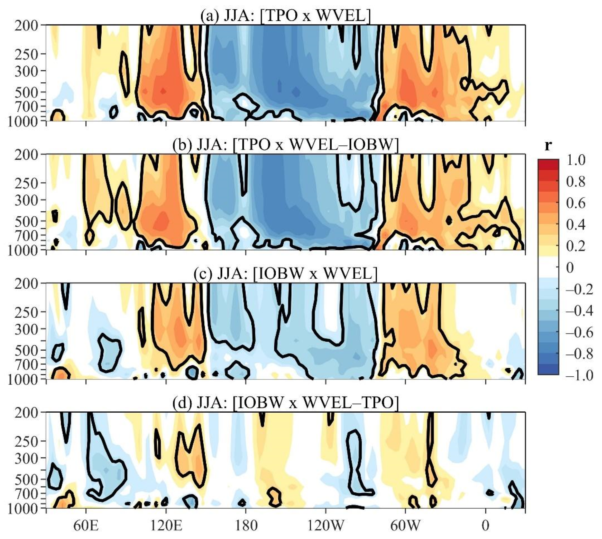
Figure 5 illustrates the longitude vertical cross-sections of the total and partial correlations for the WVEL. Significant [TPO × WVEL] correlations appear in most tropospheric levels with the negative ones in the central and eastern Pacific (150° E–75° W) flanked by positive correlations to the east between the eastern Pacific and the Atlantic (75° W–0° W) and to the west in the western Pacific (105° E–150° E) (Figure 5a). For positive TPO, there is an eastward-displaced Walker cell associated with EN occurrences [29], such that negative correlations reflect anomalous rising motions, and the positive ones, anomalous sinking motions. Similar features are observed for the [TPO × WVEL minus IOBW] correlations, except for positive correlations in larger bands, with the band in the western Pacific extending to the central Indian Ocean in the middle and upper tropospheric levels and that in the eastern Pacific/Atlantic, extending to western Africa (0° E–30° E) in lower to upper tropospheric levels (Figure 5b). Therefore, when the warm IOBW effect is removed, the EN-induced sinking motions are intensified over the Indian and western African longitudes.

For positive IOBW, the [IOBW × WVEL] correlations describe an anomalous tripolar Walker cell, with sinking motions in most tropospheric levels in the western Pacific (110° E–150° E) and South American/Atlantic (80° W–15° W) bands and in the lower-tropospheric levels in the equatorial-western Indian Ocean, and rising motions in the lower to middle tropospheric levels of the eastern Indian Ocean/Indonesia (80° E–90° E) and in most equatorial longitudes of the Pacific Ocean (Figure 5c). The corresponding partial correlations when the EN effect is removed feature anomalous rising motions in a larger longitudinal band of the Indian Ocean/Indonesia (60° E–90° E), and in two narrow bands, one in the eastern Pacific/South America (100° W–90° W) and another in Africa, and anomalous sinking motions in the middle and upper tropospheric levels of the western Pacific (120° E–150° E) (Figure 5d). In this case, it is noteworthy that the sinking motions over the South American/Atlantic sector are reduced (Figure 5d). When the EN effect is removed, the warm IOBW event favors a tripolar east-west cell with its rising motions approximately in the longitudes of the climatological tropical convection [30] and sinking motions in the western Pacific (130° E–140° E) where is a climatologically upwelling region (Figure 5d). For positive IOBW, the branches of the tripolar east-west cells inferred from the [IOBW × WVEL] and [IOBW × WVEL minus TPO] correlations show nearly coincident positions, except for some differences in their longitudinal and/or vertical extensions (Figure 5c,d).

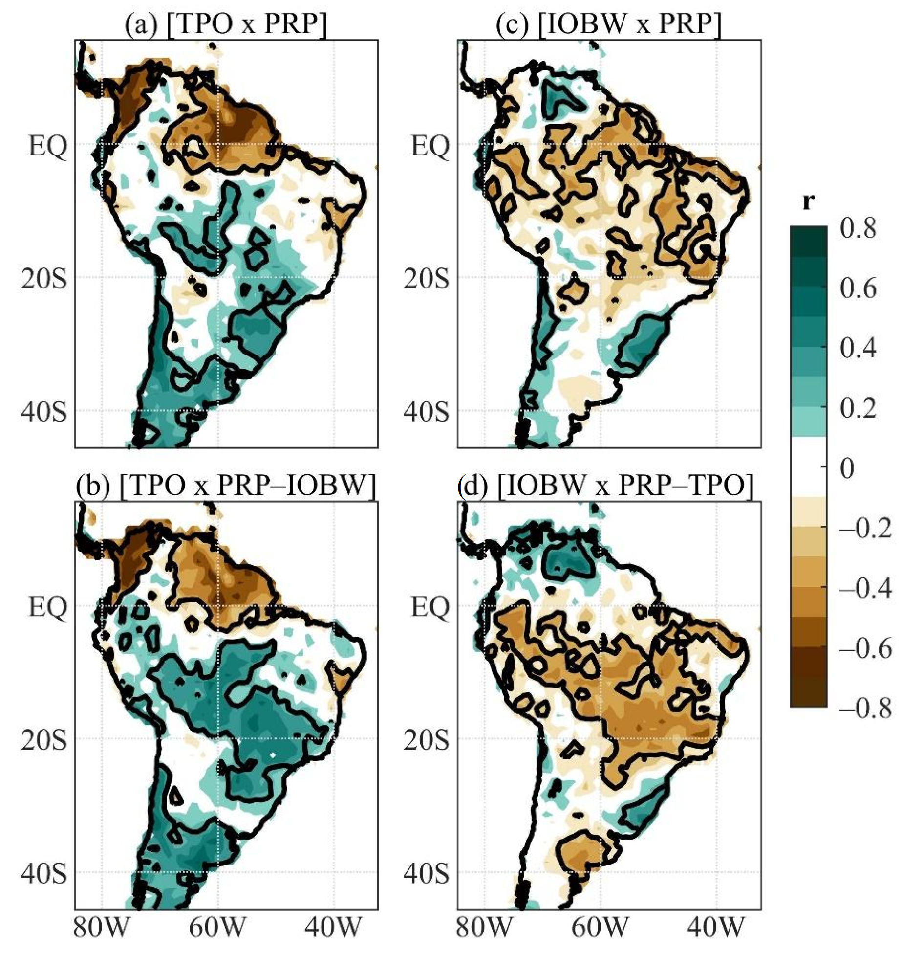
In order to examine the effects of the vertical velocity anomalies over the South American climate, correlation maps were also obtained for precipitation. The [TPO × PRP] and [TPO × PRP minus IOBW] correlation maps show similar patterns, except for well-organized positive partial correlations in central and eastern South America (Figure 6a,b). The following interpretation of the correlations refers to the positive TPO. The correlation patterns represent the EN-related precipitation deficits in northwestern and northern South America and excessive rainfall in SESA and are consistent with previous findings [13,14]. On the other hand, the significant positive correlations in central and eastern South America represent EN-related positive precipitation anomalies, but their magnitudes might not be large because these regions are under the dry season. The precipitation deficits in equatorial South America are closely linked to the EN-related significant anomalous sinking motions in these longitudes, which are associated with an eastward-displaced Walker cell (Figure 5a,b, Figure 6a,b). These results are consistent with earlier findings on the EN effects on rainfall in equatorial South America [13]. The excessive rainfall in SESA was previously attributed to the EN-related intensified subtropical jet stream [9,10].

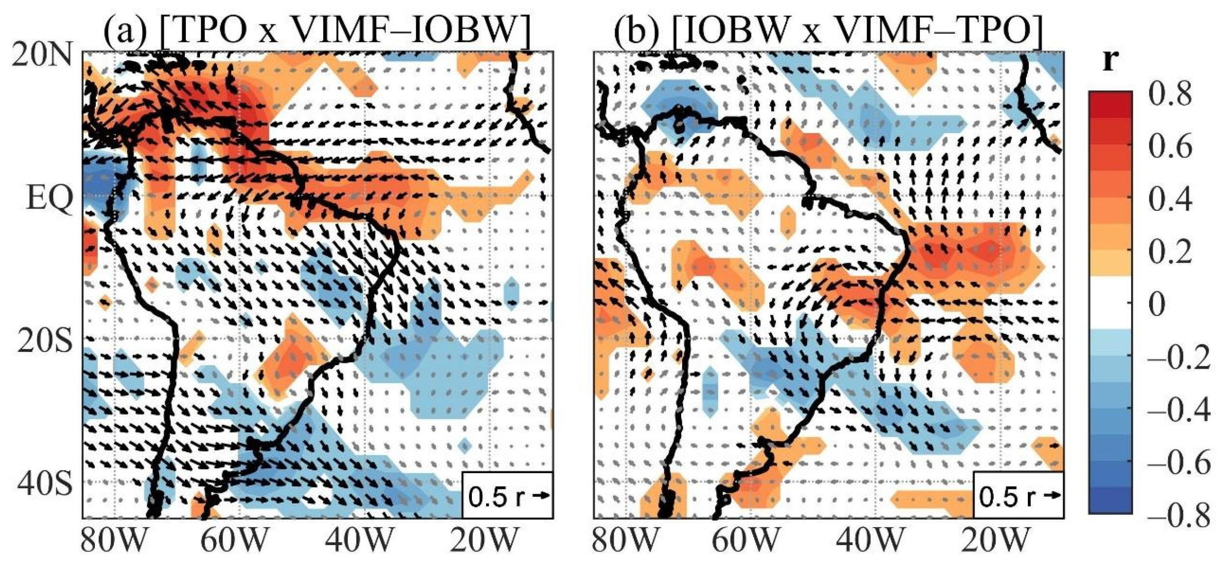
Connections between the regional circulation and rainfall anomalies during winter are examined here using the VIMF components and their divergence. The total and partial correlations show similar patterns, so only partial correlations are presented. For positive TPO, the [TPO × VIMF minus IOBW] correlation map represents a moisture divergent flow in the TNA and northern South America, where it splits into three parts, one continues westward, another curves northwestward, and the last one blows southeastward over the sector between the equator and 20° S (Figure 7a). In addition, a flow in the southeastern Pacific blows southeastward in central-western South America between 20° S and 40° S, crosses SESA, and converges with the flow coming from the Amazon in southern Brazil and Uruguay (Figure 7a). In addition, two anticyclones in the tropical South Atlantic (TSA), one centered at (30° S, 20° W) and another off the NEB coast, are evident (Figure 7a). Considering the positive TPO, the partial correlation map indicates moisture convergence over SESA and the continental sector between 5° S and 20° S (Figure 7a).

The [IOBW × PRP] map shows significant negative correlations in scattered areas of South America north of 20° S, except for central Venezuela, and positive ones in southern Brazil and along the western coast of subtropical South America (Figure 6c). Moreover, the [IOBW × PRP minus TPO] map shows well-organized negative correlations in an extensive area between the equator and 25° S in central and eastern South America and an area in eastern Argentina centered at (38° S, 65° W), and the positive correlations over central and northern Venezuela and in a small area of southern Brazil (Figure 6c,d). Regarding the warm IOBW phase, the [IOBW × VIMF minus TPO] correlation map represents a moisture divergent flow in the equatorial Atlantic, splitting into two branches, one northward into the TNA, and another crossing NEB, where in association with an anticyclone in TSA it acquires an anticyclonic curvature and reaches central-eastern Brazil (Figure 7b). Still, for the positive IOBW, a southeastward flow transports moisture from the southwestern Amazon into southern and southeastern Brazil, where moisture convergence is noted (Figure 7b). Regarding the warm IOBW, centers of moisture divergence appear in the Amazon, southern NEB, and the southwest Atlantic off the Argentinian coast.

The regional atmospheric circulations inferred from the partial correlations between the oceanic indices and the VIMF components and their divergence in some regions contribute to defining the rainfall anomaly patterns, such that negative precipitation anomalies are related to the moisture divergence and positive precipitation anomalies, to the moisture convergence. Consistent relationships between [TPO × PRP minus IOBW] and [TPO × VIMF minus IOBW] are conspicuous in northern South America and SESA (Figure 6b and Figure 7a). For the [IOBW × PRP minus TPO] and [IOBW × VIMF minus TPO] maps, consistent relationships are more evident in areas of central South America between 5° S and 15° S (Figure 6d and Figure 7b). Nevertheless, the partial correlations for the VIMF components and their divergence and for the precipitation do not show consistent relations in some areas. This is particularly noticeable in the inner side of southeastern Brazil where the significant positive [TPO × PRP minus IOBW] and [TPO × VIMF minus IOBW] correlations do not combine, and neither the significant negative [IOBW × PRP minus TPO] and [IOBW × VIMF minus TPO] correlations (Figure 6b,d and Figure 7a,b). In addition, in the South American band between 5° S and 15° S, the anomalous westerly flow relates to positive precipitation anomalies for the positive TPO, and IOBW the anomalous easterly flow relates to negative precipitation anomalies for the warm IOBW (Figure 6b,d and Figure 7a,b). These relationships between the zonal winds and rainfall variations in central-western Brazil during winter, which is the dry season in this region, have correspondences with the previously shown dry and wet periods within the wet season of this same region [31].

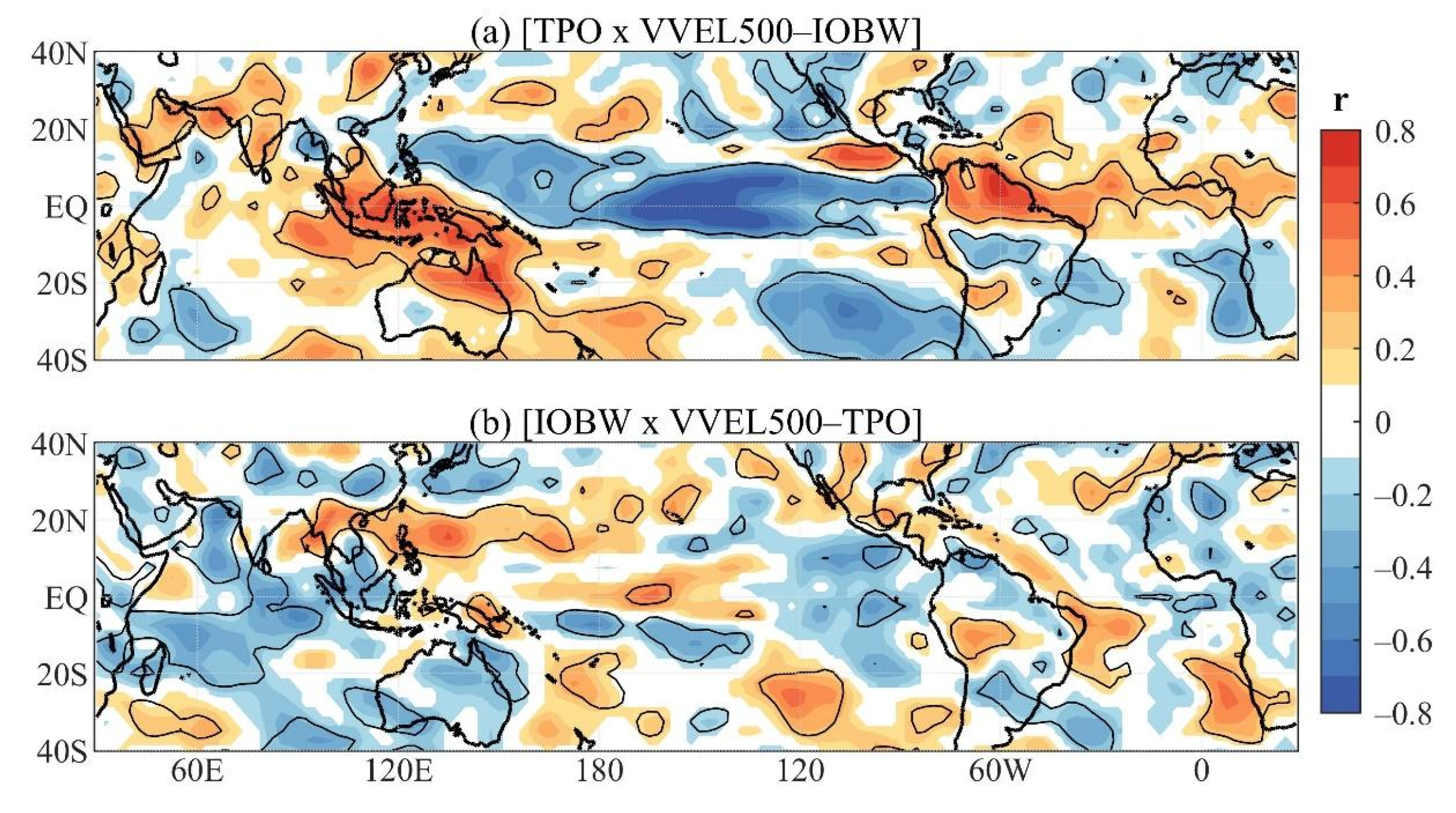
The contrasting patterns of the [TPO × PRP minus IOBW] and [IOBW × PRP minus TPO] maps (Figure 6b,d), particularly conspicuous in central and eastern South America, suggest that the regional Hadley cell might also contribute to these differences. The [TPO × VVEL500 minus IOBW] map shows significant positive correlations over South America to the north of 5° S and the adjacent Atlantic Ocean and the negative ones over the equatorial Pacific, which for positive TPO represent an anomalously eastward-shifted Walker cell associated with the EN (Figure 8a). This map also shows negative correlations between 5° S and 20° S in most of central and eastern South America and positive correlations between 20° S and 30° S over central-western South America (Figure 8a). Consistent relationships between the positive [TPO × PRP minus IOBW] correlations and negative [TPO × VVEL500 minus IOBW] correlations, and vice versa, can be interpreted in terms of the circulation and rainfall anomalies. For the positive TPO, the anomalous sinking motions relate to the negative precipitation anomalies in an extensive area in northern South America (northern Brazil, Venezuela, Guiana, Suriname, and French Guiana), and anomalous rising motions in central and eastern South America, the positive precipitation anomalies in this area (Figure 6b and Figure 8a). 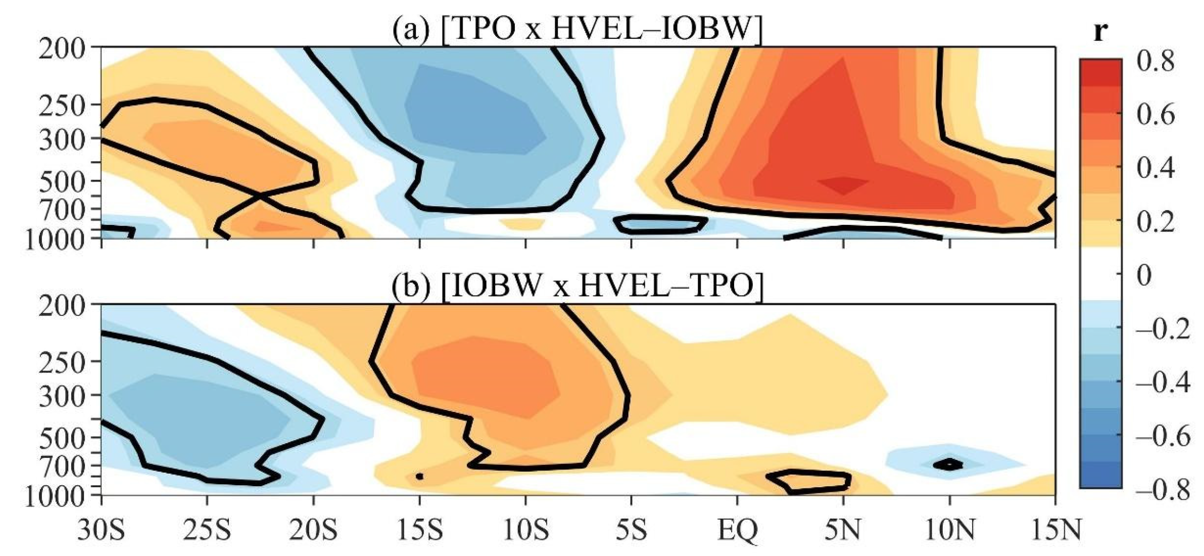The consistent vertical velocity and precipitation relations are also illustrated with the averaged vertical velocities along 60° W (Figure 9a). In this case, the latitude vertical cross-section of the [TPO × HVEL minus IOBW] panel shows in most tropospheric levels significant positive correlations in the 15° N–5° S and 20° S–30° S bands, and significant negative correlations in the 7.5° S–17.5° S band (Figure 9a). For positive TPO, these correlations represent an anomalous regional Hadley cell and are consistent with a dipole-like pattern between northern and central and eastern South America in the corresponding partial correlations of the TPO and precipitation (Figure 6a and Figure 9a).

On the other hand, the [IOBW × VVEL500 minus TPO] map shows significant negative correlations in northernmost South America and in an area including southern Bolivia, northern Argentina, Paraguay, and southern Brazil, and the positive ones in the band between 5° S and 20° S, which are better defined in central-western South America, and over coastal areas of NEB (Figure 8b). In this case, the consistent relations between the [IOBW × VVEL500 minus TPO] and [IOBW × PRP minus TPO] correlations occur in northernmost South America, in the area between 5° S and 20° S in central-western South America and in coastal southern Brazil (Figure 6d and Figure 8b). It is remarkable that most of the extensive area with negative [IOBW × PRP minus TPO] correlations in central-eastern South America does not show positive [IOBW × VVEL500 minus TPO] correlations (Figure 6d and Figure 8b). This result indicates that the correlation analysis should be taken with caution. In particular, the negative [IOBW × PRP minus TPO] correlations in easternmost South America might not represent large magnitude precipitation anomalies. In addition, the latitude vertical cross-section of the [IOBW × HVEL minus TPO] correlations show almost opposite sign values to those for the [TPO × HVEL minus IOBW] correlations, while the negative correlations to the north of 5° S are not well-defined (Figure 9a,b).

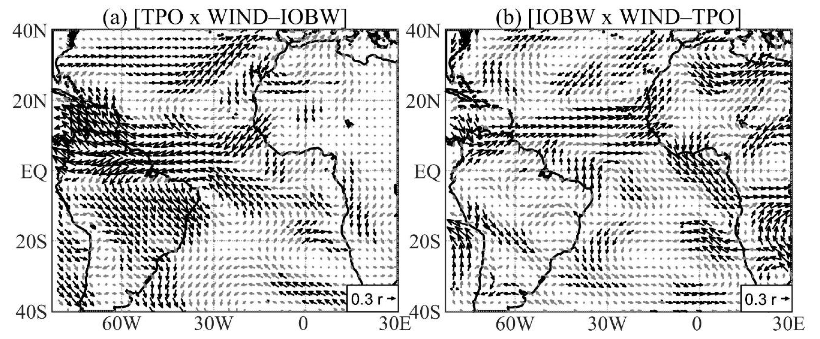
The [TPO × WIND minus IOBW] map shows similar patterns as those for the [TPO × VIMF minus IOBW] and for the positive TPO it depicts an intensified South Atlantic subtropical high-pressure system, which is typical of EN, and two anomalous anticyclones, one centered at (20° N, 30° W), and another over NEB and the adjacent Atlantic, and between them accelerated trade winds along the equatorial Atlantic (Figure 10a). On the other hand, [IOBW × WIND minus TPO] and [IOBW × VIMF minus TPO] show similar features with a quite complex horizontal structure with several vortexes over the study domain (Figure 7b and Figure 10b). For positive IOBW, the most outstanding feature is the dominance of anomalous westerlies in the tropical Atlantic band between 20° N and 5° N (Figure 10b).

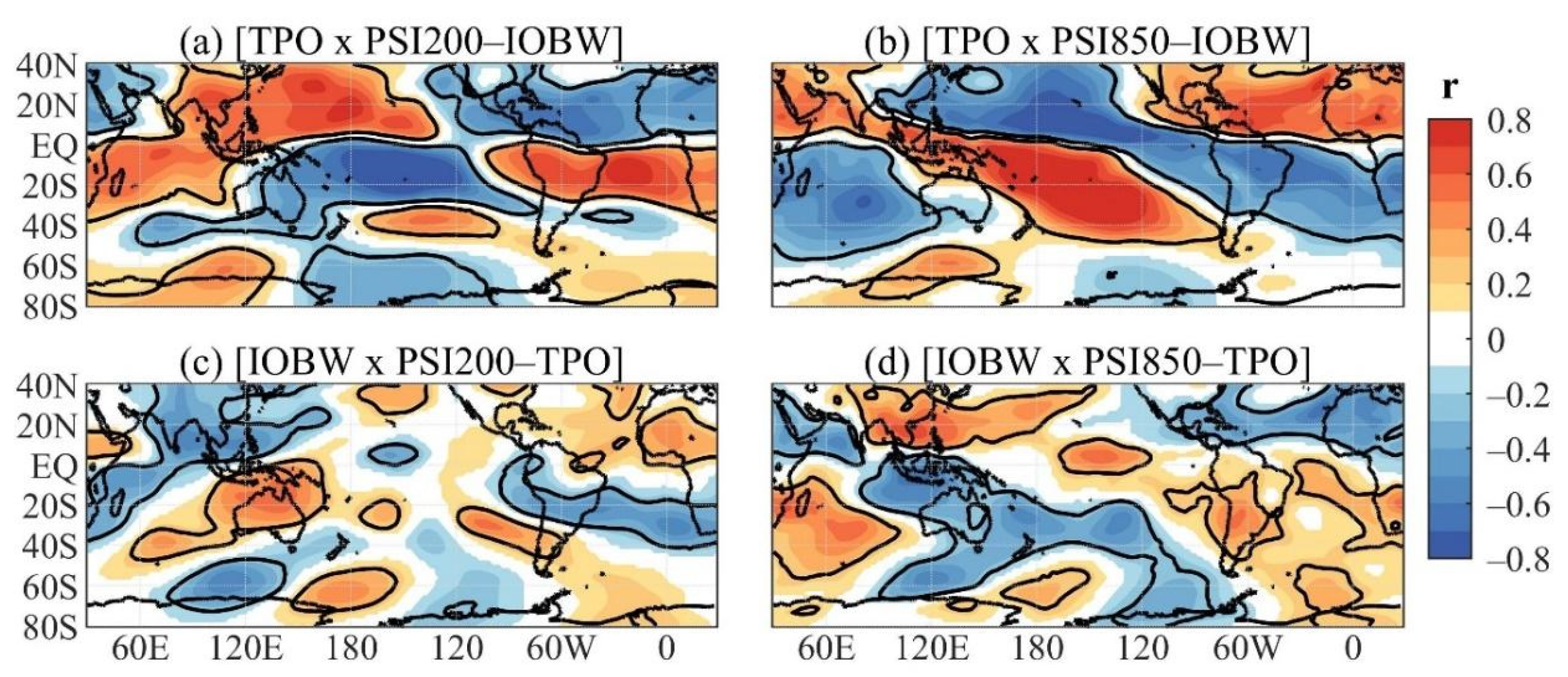
As for the other variables, only the partial correlation maps for the 200 hPa and 850 hPa asymmetric streamfunction are examined. Correlations in the two levels show centers with opposite signs in the tropics and the same sign in the subtropics and extratropics, which for a given phase of the mode (TPO or IOBW) can be interpreted as circulation pattern with baroclinic structure in the tropics and nearly equivalent barotropic structure in the subtropics and extratropics (Figure 11) [32]. For the EN without the warm IOBW event effect, the 200 hPa tropical circulation reflects the theoretical atmospheric response to the equatorial Pacific warming with an anomalous anticyclone in the central-western Pacific and anomalous cyclones in the Indo-Asian and the South American/Atlantic/African regions (Figure 11a) [33,34]. In addition, for the EN, the Pacific-South American (PSA) teleconnection pattern is evident and has an equivalent barotropic anticyclone in subtropical South Atlantic, which is consistent with the moisture transport into SESA (Figure 6b, Figure 7a and Figure 11a,b). On the other hand, the [IOBW × PSI200 minus TPO] and [IOBW × PSI850 minus TPO] maps illustrate centers of alternated sign correlations connecting the Indo-western Pacific Ocean and South America through the extratropical Southern Hemisphere (Figure 11c,d). For the positive IOBW, this pattern represents an anomalous anticyclone over the Bellingshausen Sea and an anomalous cyclone over SESA (Figure 11c,d). The cyclone over SESA contributes to the moisture transport into southern Brazil (Figure 6d, Figure 7b and Figure 11c,d).

A careful comparison of the [TPO × PSI850 minus IOBW] and [IOBW × PSI850 minus TPO] correlation maps indicates that the tropical patterns have a phase difference of approximately 90° in longitude such that over South America, these maps show reversed sign correlations, which for positive TPO and positive IOBW represent, respectively, an anomalous anticyclone centered in eastern South America and anomalous cyclone centered over subtropical South America (Figure 11b,d). This might be the main cause of the differences in the rainfall anomalies over South America associated with the EN and warm IOBW events (Figure 6b,d).

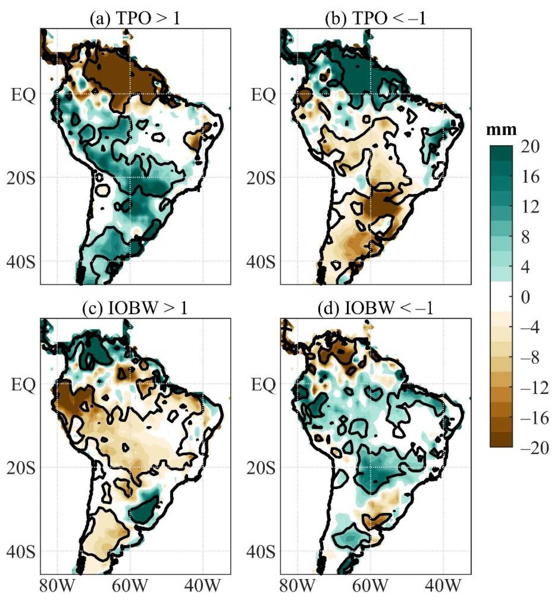
Since previous studies have shown little winter precipitation in central-eastern South America, approximately between 5° S and 25° S [15], and the amount of rainfall anomalies can not be inferred from correlation maps, the ENSO and IOBW impacts on precipitation are examined further with composite analyses. Residual oceanic indices and the corresponding residual precipitation anomalies without standardization (mm/month) are used in these analyses. In the composite analyses, six years were included for the TPO > 1 composite and eight years for the other composites (TPO < −1, IOBW > 1, and IOBW < −1). The precipitation composites show non-linearities in some areas for both oceanic indices, more accentuated for the IOBW index. The TPO > 1 composite shows a rainfall anomaly pattern very similar to the [TPO × PRP minus IOBW] map when considering the EN event, with the largest anomalies exceeding 10 mm/month in magnitude in northern South America, SESA, and in areas of central and central-eastern South America (Figure 6b and Figure 12a). The TPO < −1 composite features a nearly reversed sign precipitation anomaly pattern, but with the largest anomalies exceeding 15 mm/month in magnitude in northern South America, inner southeastern Brazil, and part of the Mato Grosso do Sul state (approximately between 22° S and 30° S to the east of 60° W) (Figure 12b). This explains the inconsistency between [TPO × PRP minus IOBW] and [TPO × VIMF minus IOBW] in inner southeastern Brazil (Figure 6b and Figure 7a). In addition, negative precipitation anomalies exceeding 10 mm/month in magnitude are found in small areas of central-western South America (Figure 12b).

For the IOBW > 1 composite, negative anomalies are found in an extensive area in the equator-25° S band and west of SESA. The positive ones are in northern Colombia, western Venezuela, western Uruguay, and southern Brazil (Figure 12c). For the IOBW < −1 composite, positive precipitation anomalies are noted in a small area in central-eastern Argentina and areas in the equator-25° S band, and the negative ones in Venezuela, a small area in western Uruguay and central-eastern Argentina (Figure 12d). Concerning the pattern of the [IOBW × PRP minus TPO] correlations for the warm IOBW event, the precipitation anomaly pattern of the IOBW > 1 composite presents similar features in the equator-30° S band, and the centers in northern South America and SESA are slightly westward positioned (Figure 6d and Figure 12c). A similar comparison between the [IOBW × PRP minus TPO] correlations for the negative IOBW event and the IOBW < −1 composite indicates almost coincident positions of the anomaly centers in northern South America and SESA (Figure 6d and Figure 12d). For the IOBW > 1 composite, the negative precipitation anomalies to the east of 50° W in the 5° S–15° S band are quite reduced, and for the IOBW < −1 composite, the expressive positive anomalies are found in small scattered areas to the northwest of the equator-25° S band, in the 15° S–25° S band in central South America and along the northern Brazil coast between 50° W and 40° W (Figure 12d). These results indicate that the partial correlations of the IOBW and precipitation can be considered for practical application, except in the area between 5° S and 15° S and east of 50° W (Figure 6d and Figure 12c,d).

4. Discussions and Conclusions

The present paper examines the relative role of the ENSO and IOBW modes in the southern winter rainfall interannual variability over South America using gridded reanalyzed data of the 1951–2016 period: the atmospheric circulation data from NCEP/NCAR Reanalysis-I, GPCC precipitation data, and the SST data from NOAA The PC time series of the dominant EOF modes of the SST anomalies in the tropical Indian and Pacific Oceans are used to describe the IOBW and ENSO modes, and are referred to, respectively, as IOBW and TPO indices. Analyses are based on total and partial correlations.

For the positive TPO index, the partial correlations between the TPO index and the atmospheric circulation variables, when the warm IOBW event effect is removed describe global and regional atmospheric circulation anomalies previously imputed to the EN events, which feature: an anomalous eastward-shifted Walker cell [29]; the Matsuno–Gill atmospheric response to the tropical Pacific heating [33,34], and intensified low-level northwesterly winds across central-western South America (Figure 5b, Figure 7a, Figure 10a and Figure 11a,b) [1]. Consequently, the partial correlation between the TPO and precipitation shows significant negative correlations in northwestern-northern South America and the positive ones in SESA, representing a typical EN-related precipitation anomaly pattern for positive TPO index (Figure 6b) [13]. The significant positive partial correlations between the TPO and precipitation in an extensive area of central and eastern South America are concordant with negative partial correlations between the TPO and HVEL in the 7.5° S–17.5° S band (Figure 6b and Figure 9a). For positive TPO, these correlations indicate that the excessive rainfall in central and eastern South America is also related to an anomalous regional Hadley cell with rising motions in the 7.5° S–17.5° S band and sinking motions to the north of 5° S (Figure 6b and Figure 9a). This result confirms previous findings on the role of the EN-related changes in the regional Hadley cell [1]. Furthermore, the significant positive correlations in central and eastern South America are better organized when the warm IOBW event effect is removed (Figure 6a,b). This result implies that the warm IOBW event has a drying effect in this region, clearly illustrated in the [IOBW × PRP minus TPO] correlation map (Figure 6d). Since the warm IOBW and EN events co-exist [19], their opposite effects on central and eastern South America explain why the EN signature in the rainfall in this region cannot be clearly identified during most events.

When the EN event effect is removed, the partial correlations between the IOBW index and the analyzed variables exhibit distinct patterns from those mentioned above for the TPO index. In fact, for the warm IOBW event, the east-west circulation along the vertical-equatorial plane features a tripolar structure with rising branches co-positioned with climatological tropical convective areas and reduced positive correlations in the South American/Atlantic sector (Figure 5d). Therefore, the warm IOBW event might play an important role in tropical South American precipitation. This aspect is more evident for the [IOBW × HVEL minus TPO] correlations. For the warm IOBW event, there is an anomalous meridional cell with sinking motions in the 5° S–20° S band and rising motions in the 20° S–30° S band (Figure 9b). This meridional cell has consistent relationships with the rainfall anomalies in tropical South America, as indicated by the composite analyses (Figure 6d and Figure 12).

One of the most relevant results of the present analysis refers to the contrasting effects of EN and warm IOBW events on the rainfall in tropical South America, when their effects are isolated from each other (Figure 6b,d). The contrast is even more remarkable in central and eastern (between 5° S and 25° S) South America, such that EN relates to the anomalous wet conditions, and the warm IOBW to the anomalous dry conditions (Figure 6b,d). These effects result primarily from the anomalous regional Hadley cells with opposite circulation patterns in the 5° S–15° S band (Figure 9a,b). In addition, [TPO × PSI850 minus IOBW] and [IOBW × PSI850 minus TPO] correlation maps show tropical patterns with a phase difference of approximately 90° in longitude, which for positive TPO and warm IOBW events feature, respectively, an anomalous anticyclone centered in eastern South America and an anomalous cyclone centered over subtropical South America (Figure 11b,d). These circulation anomalies might be the main cause of the differences in the rainfall anomalies over subtropical South America associated with the EN and warm IOBW events (Figure 6b,d).

The most outstanding result here is that the warm IOBW and EN events, when their effects are isolated from each other, have opposite effects on the winter rainfall, particularly in central and eastern (between 15° S and 25° S) South America. To the best knowledge of the authors, the results presented here have not been discussed previously. We believe that the results presented in this analysis may be further assessed by future modeling studies and using other reanalysis datasets.

References

1. Zhou, J.; Lau, K.M. Principal modes of interannual and decadal variability of summer rainfall over South America. Int. J. Climatol. 2001, 21, 1623–1644. [Google Scholar] [CrossRef]
2. Mo, K.C.; Higgins, R.W. The Pacific-South American modes and tropical convection during the Southern Hemisphere winter. Mon. Weather Rev. 1998, 126, 1581–1596. [Google Scholar] [CrossRef]
3. Paegle, J.N.; Mo, K.C. Linkages between summer rainfall variability over South America and sea surface temperature anomalies. J. Clim. 2002, 15, 1389–1407. [Google Scholar] [CrossRef] [Green Version]
4. Ropelewski, C.F.; Halpert, M.S. Global and Regional scale precipitation patterns associated with the El Niño-Southern Oscillation. Mon. Weather Rev. 1987, 115, 1606–1626. [Google Scholar] [CrossRef] [Green Version]
5. Kousky, V.E.; Ropelewski, C.F. Extremes in the Southern Oscillation and their Relationship to Precipitation Anomalies with Emphasis on the South American Region. Rev. Bras. Meteorol. 1989, 4, 351–363. [Google Scholar]
6. Aceituno, P. On the Functioning of the Southern Oscillation in the South American Sector. Part I: Surface Climate. Mon. Weather Rev. 1988, 116, 505–524. [Google Scholar] [CrossRef] [Green Version]
7. Kayano, M.T.; Rao, V.B.; Moura, A.D. Tropical circulations and the associated rainfall anomalies during two contrasting years. J. Climatol. 1988, 8, 477–488. [Google Scholar] [CrossRef] [Green Version]
8. Rao, V.B.; Hada, K. Characteristics of rainfall over Brazil: Annual variations and connections with the Southern Oscillation. Theor. Appl. Climatol. 1990, 42, 81–91. [Google Scholar] [CrossRef]
9. Grimm, A.M.; Ferraz, S.E.T.; Gomes, J. Precipitation Anomalies in Southern Brazil Associated with El Niño and La Niña Events. J. Clim. 1998, 11, 2863–2880. [Google Scholar] [CrossRef] [Green Version]
10. Grimm, A.; Barros, V.; Doyle, M. Climate Variability in Southern South America Associated with El Niño and La Niña Events. J. Clim. 2000, 13, 35–58. [Google Scholar] [CrossRef]
11. Grimm, A.M. The El Niño Impact on the Summer Monsoon in Brazil: Regional Processes versus Remote Influences. J. Clim. 2003, 16, 263–280. [Google Scholar] [CrossRef]
12. Grimm, A.M. How do La Niña events disturb the summer monsoon system in Brazil? Clim. Dyn. 2004, 22, 123–138. [Google Scholar] [CrossRef]
13. Grimm, A.M. Interannual climate variability in South America: Impacts on seasonal precipitation, extreme events, and possible effects of climate change. Stoch. Environ. Res. Risk Assess. 2011, 25, 537–554. [Google Scholar] [CrossRef]
14. Tedeschi, R.G.; Grimm, M.; Cavalcanti, I.F.A. Influence of Central and East ENSO on precipitation and its extreme events in South America during austral autumn and winter. Int. J. Climatol. 2016, 36, 4797–4814. [Google Scholar] [CrossRef]
15. Cai, W.; McPhaden, M.J.; Grimm, A.M.; Rodrigues, R.R.; Taschetto, A.S.; Garreaud, R.D.; Dewitte, B.; Poveda, G.; Ham, Y.-G.; Santoso, A.; et al. Climate impacts of the El Niño–Southern Oscillation on South America. Nat. Rev. Earth Environ. 2020, 1, 215–231. [Google Scholar] [CrossRef]
16. Drumond, A.D.M.; Ambrizzi, T. The role of the South Indian and Pacific oceans in South American monsoon variability. Theor. Appl. Climatol. 2008, 94, 125–137. [Google Scholar] [CrossRef]
17. Taschetto, A.S.; Ambrizzi, T. Can Indian Ocean SST anomalies influence South American rainfall? Clim. Dyn. 2012, 38, 1615–1628. [Google Scholar] [CrossRef] [Green Version]
18. Chambers, D.P.; Tapley, B.D.; Stewart, R.H. Anomalous warming in the Indian Ocean coincident with El Niño. J. Geophys. Res. Ocean. 1999, 104, 3035–3047. [Google Scholar] [CrossRef]
19. Lau, N.C.; Nath, M.J. Atmosphere-ocean variations in the Indo-Pacific sector during ENSO episodes. J. Clim. 2003, 16, 3–20. [Google Scholar] [CrossRef]
20. Deser, C.; Alexander, M.A.; Xie, S.P.; Phillips, A.S. Sea Surface Temperature Variability: Patterns and Mechanisms. Ann. Rev. Mar. Sci. 2010, 2, 115–143. [Google Scholar] [CrossRef] [Green Version]
21. Kayano, M.T.; Andreoli, R.V.; Cerón, W.L.; Souza, R.A.F. The Role of the Indian Ocean Basin-Wide and El Niño—Southern Oscillation Modes in Interannual Rainfall Variability over South America during Austral Summer. Atmosphere 2021, 12, 1094. [Google Scholar] [CrossRef]
22. Kalnay, E.; Kanamitsu, M.; Kistler, R.; Collins, W.; Deaven, D.; Gandin, L.; Iredell, M.; Saha, S.; White, G.; Woollen, J.; et al. The NCEP/ NCAR reanalysis project. Bull. Am. Meteor. Soc. 1996, 77, 437–471. [Google Scholar] [CrossRef] [Green Version]
23. Schneider, U.; Becker, A.; Finger, P.; Meyer-Christoffer, A.; Ziese, M.; Rudolf, B. GPCC’s new land surface precipitation climatology based on quality-controlled in situ data and its role in quantifying the global water cycle. Theor. Appl. Climatol. 2014, 115, 15–40. [Google Scholar] [CrossRef] [Green Version]
24. Huang, B.; Thorne, P.W.; Banzon, V.F.; Boyer, T.; Chepurin, G.; Lawrimore, J.H.; Menne, M.J.; Smith, T.M.; Vose, R.S.; Zhang, H.M. Extended reconstructed Sea surface temperature, Version 5 (ERSSTv5): Upgrades, validations, and intercomparisons. J. Clim. 2017, 30, 8179–8205. [Google Scholar] [CrossRef]
25. Peixoto, J.P.; Oort, A.H. Physics of Climate; MIT Press: San Diego, CA, USA, 1992; ISBN 7287064. [Google Scholar]
26. Torrence, C.; Compo, G.P. A Practical Guide to Wavelet Analysis Christopher. Bull. Am. Meteorol. Soc. 1998, 97, 61–78. [Google Scholar] [CrossRef] [Green Version]
27. North, G.L.; Bell, T.L.; Chalan, R.F. Sampling Errors in the Estimation of Empirical Othogonal Functions. Mon. Weather Rev. 1982, 110, 699–706. [Google Scholar] [CrossRef]
28. Panofsky, H.G.; Brier, G.W. Some Applications of Statistics to Meteorology; Pennsylvania State University: State College, PA, USA, 1968. [Google Scholar]
29. Kousky, V.E.; Kagano, M.T.; Cavalcanti, I.F.A. A review of the Southern Oscillation: Oceanic-atmospheric circulation changes and related rainfall anomalies. Tellus A 1984, 36, 490–504. [Google Scholar] [CrossRef] [Green Version]
30. Rasmusson, E.M.; Arkin, P.A. A global view of large-scale precipitation variability. J. Clim. 1993, 6, 1495–1522. [Google Scholar] [CrossRef] [Green Version]
31. Gan, M.A.; Kousky, V.E.; Ropelewski, C.F. The South America Monsoon circulation and its relationship to rainfall over west-central Brazil. J. Clim. 2004, 17, 47–66. [Google Scholar] [CrossRef] [Green Version]
32. Held, I.M.; Panetta, R.L.; Pierrehumbert, R.T. Stationary external rossby waves in vertical shear. J. Atmos. Sci. 1985, 42, 865–883. [Google Scholar] [CrossRef] [Green Version]
33. Matsuno, T. Quasi-Geostrophic Motions in the Equatorial Area. J. Meteorol. Soc. Japan. Ser. II 1966, 44, 25–43. [Google Scholar] [CrossRef] [Green Version]
34. Gill, A.E. Some simple solutions for heat-induced tropical circulation. Q. J. R. Meteorol. Soc. 1980, 106, 447–462. [Google Scholar] [CrossRef]
Figure 1. Study area and tropical Indian and Pacific Ocean regions used.
Atmosphere 12 01605 g001
Figure 2. Austral winter rainfall climatology (mm).
Atmosphere 12 01605 g002
Figure 3. Seasonal spatial loading patterns and principal component time series of the first SST anomaly modes computed for the 1951–2016 period in the tropical oceanic sectors: (a) Indian Ocean during southern winter; (b) Principal component of the Indian Ocean EOF1; (c) tropical Pacific Ocean during southern winter; and (d) Principal component of the Pacific Ocean EOF1. Continuous contours encompass the significant correlations at a 95% confidence level using the Student’s t-test.
Atmosphere 12 01605 g003
Figure 4. Partial correlations for the SST during the southern winter: (a) [TPO × SST minus IOBW]; and (b) [IOBW × SST minus TPO]. Continuous contours encompass significant correlations at a 95% confidence level using the Monte Carlo method with 1000 simulations.
Atmosphere 12 01605 g004
Figure 5. Longitude vertical cross-sections of the total and partial correlations for the vertical velocity in pressure coordinate (WVEL) during the southern winter: (a) [TPO × WVEL]; (b) [TPO × WVEL minus IOBW]; (c) [IOBW × WVEL]; and (d) [IOBW × WVEL minus TPO]. Continuous contours encompass significant correlations at a 95% confidence level using the Monte Carlo method with 1000 simulations. The vertical pressure levels are in hPa.
Atmosphere 12 01605 g005
Figure 6. Total and partial correlations for the precipitation (PRP) during the southern winter: (a) [TPO × PRP]; (b) [TPO × PRP minus IOBW]; (c) [IOBW × PRP]; and (d) [IOBW × PRP minus TPO]. Continuous contours encompass significant correlations at a 95% confidence level using the Monte Carlo method with 1000 simulations.
Atmosphere 12 01605 g006
Figure 7. Partial correlations for the vertically integrated moisture flux (VIMF) components and their divergence (shades) during the southern winter: (a) [TPO × VIMF minus IOBW]; and (b) [IOBW × VIMF minus TPO]. Shades encompass significant correlations at a 95% confidence level using the Monte Carlo method with 1000 simulations. Vectors indicate the correlations with the vertically integrated moisture flux components. The arrow in the right-lower corner gives the vector base magnitude in correlation units. Bold arrows indicate vectors when at least one component has significant correlation at a 95% confidence level using the Monte Carlo method with 1000 simulations.
Atmosphere 12 01605 g007
Figure 8. Partial correlations for the 500 hPa vertical velocity (VVEL500) during the southern winter: (a) [TPO × VVEL500 minus IOBW]; and (b) [IOBW × VVEL500 minus TPO]. Continuous contours encompass significant correlations at a 95% confidence level using the Monte Carlo method with 1000 simulations.
Atmosphere 12 01605 g008
Figure 9. Latitude vertical cross-sections of the partial correlations for the vertical velocity in pressure coordinate (HVEL) during the southern winter: (a) [TPO × HVEL minus IOBW]; and (b) [IOBW × HVEL minus TPO]. Continuous contours encompass significant correlations at a 95% confidence level using the Monte Carlo method with 1000 simulations. The vertical pressure levels are in hPa.
Atmosphere 12 01605 g009
Figure 10. Partial correlations for the 850 hPa horizontal winds (WIND) during the southern winter: (a) [TPO × WIND minus IOBW] and (b) [IOBW × WIND minus TPO]. Vectors indicate correlations with horizontal winds. The arrow in the right-lower corner gives the vector base magnitude in correlation units. Bold arrows indicate vectors when at least one component has significant correlation at a 95% confidence level using the Monte Carlo method with 1000 simulations.
Atmosphere 12 01605 g010
Figure 11. Partial correlations for the asymmetric stream function during the southern winter: (a) [TPO × PSI200 minus IOBW]; (b) [TPO × PSI850 minus IOBW]; (c) [IOBW × PS200 minus TPO]; and (d) [IOBW × PSI850 minus TPO]. Continuous contours encompass significant correlations at a 95% confidence level using the Monte Carlo method with 1000 simulations.
Atmosphere 12 01605 g011
Figure 12. Composite analyses of residual precipitation anomalies in mm/month (without standardization) for: (a) TPO > 1; (b) TPO < −1; (c) IOBW > 1; and (d) IOBW < −1. Continuous contours encompass the significant values at a 95% confidence level using the Student’s t-test.
Atmosphere 12 01605 g012
Publisher’s Note: MDPI stays neutral with regard to jurisdictional claims in published maps and institutional affiliations.