
Modeling Biomass Burning Organic Aerosol Atmospheric Evolution and Chemical Aging


1
Department of Chemical Engineering, University of Patras, 26504 Patras, Greece
2
Institute of Chemical Engineering Sciences, Foundation for Research and Technology—Hellas (FORTH/ICE-HT), 26504 Patras, Greece
3
Department of Earth Science and Engineering, Imperial College London, London SW7 2AZ, UK
4
Department of Chemical Engineering, Carnegie Mellon University, Pittsburgh, PA 15213, USA
*
Author to whom correspondence should be addressed.
Atmosphere 2021, 12(12), 1638; https://0-doi-org.brum.beds.ac.uk/10.3390/atmos12121638
Submission received: 14 November 2021
/
Revised: 30 November 2021
/
Accepted: 2 December 2021
/
Published: 8 December 2021
(This article belongs to the Special Issue Secondary Organic Aerosols from Biomass Burning and Anthropogenic Precursors)
Abstract
:The changes in the concentration and composition of biomass-burning organic aerosol (OA) downwind of a major wildfire are simulated using the one-dimensional Lagrangian chemical transport model PMCAMx-Trj. A base case scenario is developed based on realistic fire-plume conditions and a series of sensitivity tests are performed to quantify the effects of different conditions and processes. Temperature, oxidant concentration and dilution rate all affect the evolution of biomass burning OA after its emission. The most important process though is the multi-stage oxidation of both the originally emitted organic vapors (volatile and intermediate volatility organic compounds) and those resulting from the evaporation of the OA as it is getting diluted. The emission rates of the intermediate volatility organic compounds (IVOCs) and their chemical fate have a large impact on the formed secondary OA within the plume. The assumption that these IVOCs undergo only functionalization leads to an overestimation of the produced SOA suggesting that fragmentation is also occurring. Assuming a fragmentation probability of 0.2 resulted in predictions that are more consistent with available observations. Dilution leads to OA evaporation and therefore reduction of the OA levels downwind of the fire. However, the evaporated material can return to the particulate phase later on after it gets oxidized and recondenses. The sensitivity of the OA levels and total mass balance on the dilution rate depends on the modeling assumptions. The high variability of OA mass enhancement observed in past field studies downwind of fires may be partially due to the variability of the dilution rates of the plumes.
1. Introduction
Particles and trace gases emitted or produced in the atmosphere have serious impacts on human health. One out of eight deaths on a global basis is currently attributed to air pollution [1], and it is estimated that worldwide 3.3 million premature deaths are due to ambient air pollution annually [2]. One of the main causes of these deaths is the exposure to elevated levels of particulate matter less than 2.5 μm in diameter (PM2.5) which leads to increased risk of cardiovascular disease [2,3]. At the same time, atmospheric particulate matter affects the optical characteristics and energy balance of the atmosphere both directly, by absorbing and scattering incoming solar radiation, and indirectly, by modifying cloud properties [4,5]. The net effect of the absorbance and reflectance of sunlight by aerosols and the effects of aerosol size and composition changes on cloud properties are the most uncertain factors in the global radiative balance [6].
Biomass burning is the most important global source of fine carbonaceous particles [7,8,9]. Biomass burning organic aerosol (bbOA) can contribute significantly to OA concentrations both near its source and far downwind [10]. The contribution of biomass burning to ambient concentrations of secondary organic aerosol (SOA) is highly uncertain, because of the complexities of the physical and chemical evolution of biomass burning plumes. After emission, changes in bbOA concentrations depend on the relative balance between evaporation of fresh biomass burning primary organic aerosol (bbPOA) driven by dilution [11] or by fragmentation reactions creating higher-volatility species, and the formation of biomass burning secondary organic aerosol (bbSOA) from the oxidation of semi-volatile (SVOCs), intermediate volatility (IVOCs) and volatile organic compounds (VOCs). The study of these changes is facilitated by normalizing the OA concentrations to a co-emitted species such as carbon monoxide (CO), assumed to be practically inert in the measurement time scales [12,13]. The normalized excess mixing ratio ΔOA/ΔCO corrects for the background concentrations of both OA and CO thus accounting for the effects of dilution. An increase in ΔOA/ΔCO implies net SOA production, whereas a decrease implies that the evaporation of POA dominates. POA and SOA predictions by our model can be used to explain the factors affecting the predicted changes of ΔOA/ΔCO over time.
Observed changes in the normalized OA concentrations downwind of biomass burning emissions after several hours appear to be highly variable [14,15]. In some biomass burning field studies, normalized OA concentrations increase downwind of the fire [16,17,18,19]. For examples measurements in southern African savannah and grassland fire plumes indicate a net increase in PM1 of more than a factor of 2, in a few hours of daytime ageing [20,21]. These are some of the highest PM enhancements in the literature, while in most other studies, the OA concentrations appear to decrease [11,12,22] or do not change significantly [13].
Several studies have simulated the evolution of bbOA downwind of specific fires [23,24], concluding that there is high variability in their evolution. May et al. [13] modeled the evolution of emissions from several prescribed burns in South Carolina. Assuming equilibrium partitioning between the gas and particulate phase they concluded that there was no statistically significant increase in OA concentrations downwind of the fire, suggesting that the evaporation of POA due to dilution balanced the formation of SOA [13]. Alvarado et al. [23] used a plume-scale Lagrangian transport model and the 1-D Volatility Basis Set (VBS) [24] representation of OA to simulate a prescribed burn in California [12]. They varied a number of model parameters in order to reproduce the observed evolution of OA and ozone (O3) in the plume. From the results of these simulation cases, the authors developed a set of reasonable revised parameters for the values of the OA aging rate (with OH), OH regeneration, split between fragmentation vs. functionalization, and O3 production. They noted that their result is sensitive to the initial bbOA volatility distribution. Bian et al. [25] performed simulations of the evolution of ambient bbOA concentrations, showing that the fire area, the mass emissions flux, and the atmospheric stability strongly modulate initial plume concentrations and plume dilution rates. They concluded that while the measured OA enhancement ratio may be close to unity, there is still significant SOA formation in these plumes which is balanced by POA evaporation. Despite this progress, the evolution of bbOA remains a significant gap in our understanding of the impact of biomass burning on both air quality and climate change [26,27].
Most modeling studies of biomass burning emissions so far have used Lagrangian parcel models, thus simplifying the treatment of the dispersion of the plume. The simulation of the particle size distribution is especially challenging due to coagulation [28]. The present study extends these efforts by using a more realistic representation of biomass burning plumes in a Lagrangian framework, simulating both vertical dispersion and horizontal dilution. By doing this, we can investigate factors that affect the evolution of biomass burning emissions and constrain the uncertain model parameters based on the predicted OA enhancement ratio [13]. The gas-phase chemistry is simplified assuming a constant OH level during the 24 h of our simulations. Nighttime processing of the biomass burning plume is neglected. The role of the OH levels, aging rates and aging chemical pathways (functionalization/fragmentation split), temperature, and dilution rates (vertical and horizontal) are investigated.
2. Model Description
In this study, the one-dimensional Lagrangian transport model of Murphy et al. [29] is used to track a column of air as it travels in space. This model is a 1-D version of the 3-D chemical transport model PMCAMx. Previous versions of this host model have been applied to California in efforts to develop predictive modules for processes such as SOA formation [30,31] and gas/particle partition. The model includes relevant atmospheric processes including gas-phase chemistry (using the Statewide Air Pollution Research Center (SAPRC) gas-phase chemistry mechanism), dry deposition, and vertical turbulent dispersion. Removal processes have been updated with treatments similar to those in PMCAMx [32]. The atmospheric diffusion equation solved by PMCAMx-Trj is:
where ci is the concentration of species i as a function of height z and time t, Kzz is the vertical eddy diffusivity which describes vertical turbulent dispersion, Ri is the chemical generation term for i, and Ei and Si are the emission and removal fluxes, respectively. The last term in (1) accounts in a simplified way for horizontal dilution where k is the horizontal dilution rate constant and ci,b the background concentration of each species i outside the simulated column of air. For our study the emissions term is set to zero and the fire plume is part of the initial conditions of the model. The 10 grids cell column reaches up to 2.5 km in the atmosphere with the first cell top boundary at 55 m. Layer heights are held constant for all simulations and are shown in Table S1 in the supplementary information. All the meteorological parameters are given as an input to the model, while anthropogenic and biogenic emissions, and wet deposition terms are assumed to be zero.
The model tracks the following OA components using the VBS [25]: (1) fresh POA; (2) anthropogenic SOA from VOCs; (3) biogenic SOA from VOCs; (4) SOA from semi-volatile and intermediate volatility organic compounds (SVOCs and IVOCs), and (5) long-range transport OA, which is considered nonvolatile due to the assumption that it has been heavily oxidized before entering the modeling domain. All OA components are represented with 12 logarithmically-spaced volatility bins of effective saturation concentrations (C*) from 10−5 to 106 μg m−3 at 298 K [29]. Therefore, the OA is simulated with 49 surrogate compounds in this application.
Model Application
In this study, a base case was first developed relying on measured fire parameters to create a realistic representation of a typical biomass burning plume. Plume conditions which are assumed to remain constant are shown in Table 1. The background concentrations are based on the reported values in Alvarado et al. [23] (Table 2). A constant moderate OH level of 5 × 10⁶ molecules cm−3 is assumed in the base case. Additionally, a low wind speed of 2 m s−1 is used, and horizontal dilution is neglected (k = 0 s−1) in the base case.
An initial plume OA concentration (CTOT) of 800 μg m−3 is injected in the seventh layer of the model (750–1000 m). This bbOA is divided into volatility bins based on the volatility distribution of May et al. [33]. An additional 1.5 CTOT is added to the C* = 104 to 106 μg m−3 volatility bins to represent IVOCs [34]. The volatility distribution of the organic emissions is shown in Table S2. Initial plume concentrations of inorganic species from Alvarado et al. [23] are divided evenly between the six modeled PM2.5 size bins as in Murphy et al. [29] and are summarized in Table 2. Aerosol species with diameters from 40 nm to 10 μm are tracked using eight logarithmically-spaced size sections. Inorganic aerosol species include ammonium, sodium, nitrate, chloride, sulfuric acid, particulate water, black carbon, and crustal species.
Layers above and below the bbOA injection layer are assumed initially to have background aerosol and gas concentrations, while 1 μg m−3 of OA (included in the most oxidized VBS bin; C* = 10−2) is added to these layers to represent background organic aerosol concentrations.
3. Simulation Results
3.1. Base Case
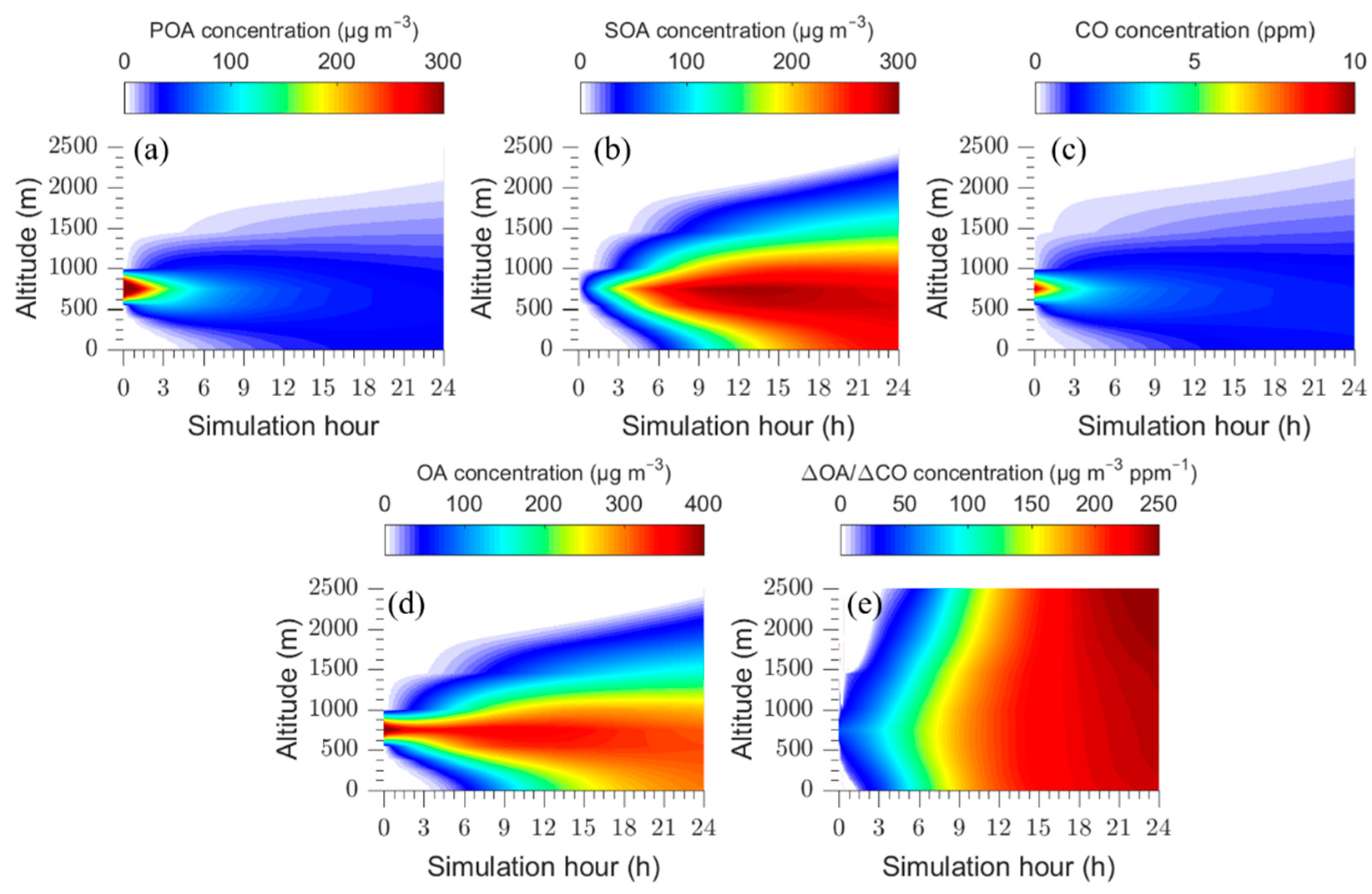
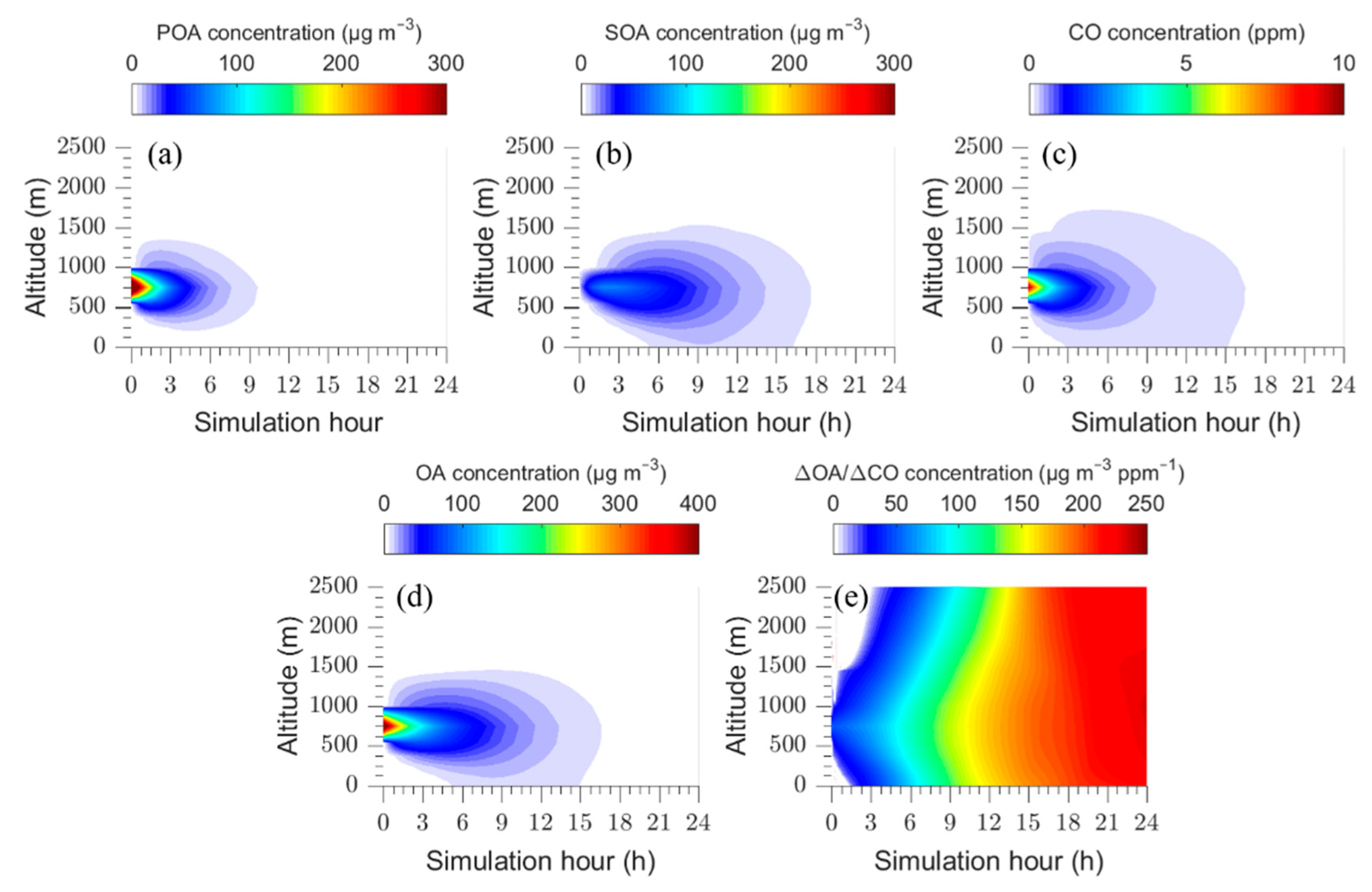
In the base case we follow the fire plume for a period of twenty-four hours. Figure 1 shows the predictions of PMCAMx-Trj for this period, as a function of altitude. The differences in the evolution of POA and CO concentrations are an indicator of the strong semi-volatile character of OA.
The concentration of POA in the plume decreases over time mainly due to its vertical dispersion and partially because of its evaporation and subsequent gas-phase oxidation. In contrast, the SOA concentration increases with time due to the oxidation of organic vapors (IVOCs and SVOCs) and the condensation of their products, reaching levels above 200 μg m−3. CO is assumed to be inert in the model and the evolution of its concentration depicts the effects of vertical dispersion of the plume. The predicted OA in the first 3 h is mainly in the form of fresh POA and its concentration is elevated at heights between 750 and 1000 m, where the plume was introduced. After these first few hours, the plume disperses and an increase in SOA concentration is predicted resulting in an increase in ΔOA/ΔCO at all levels over time. The plume remains for several hours within a narrow height range, as the base case assumes quite weak vertical mixing throughout the simulation with typical daytime OH levels that also remain constant.
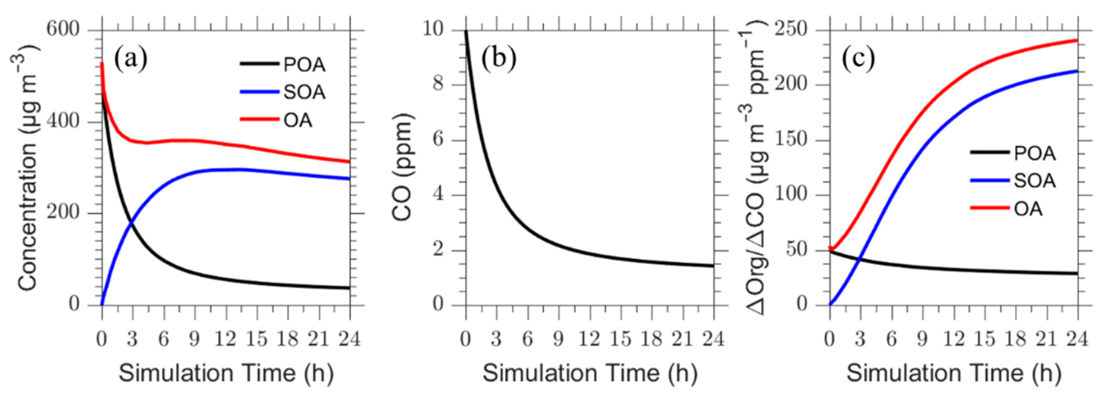
The simulation time is 24 h, without including night-time and thus represents a considerably longer period than one day of atmospheric aging. The time series for ΔOA/ΔCO, POA, SOA, CO, and total OA for the plume centerline are shown in Figure 2. The model predicts a decrease in CO concentration by approximately a factor of 7 (from 10 to 1.5 ppm) due to vertical dispersion. The primary OA concentration decreases by a factor of 14 (from 530 μg m−3 to 37 μg m−3). Part of it is due to dilution (factor of 7 same as CO) and the rest is due to evaporation. At the same time there is continuous SOA production. Predicted SOA reaches a maximum value of 300 μg m−3 after 13 h of processing in the base case scenario (Figure 2a) and then starts decreasing as dilution takes over.
The total OA decreases rapidly due to dilution of POA during the first 2 h, but then remains approximately constant for 5 h as the SOA production balances dilution and POA evaporation. After this period the OA levels continue to decrease as the SOA production has slowed down and dilution dominates again. The net change in ΔOA/ΔCO from the start of the simulation to the end is an increase of 350% (ΔOA/ΔCO = 53 μg m−3 ppm−1 in the beginning to ΔOA/ΔCO = 240 μg m−3 ppm−1 at the end). The absolute OA concentration decreases by roughly a factor of two. As several studies concentrated on the evolution of OA over shorter time periods, the corresponding predicted increase in ΔΟΑ/ΔCO over a period of 5 h is 125%.
The evolution of ΔOA/ΔCO is quite similar for the various altitudes in the modeling domain (Figure 1).
Total Biomass Burning OA Burden
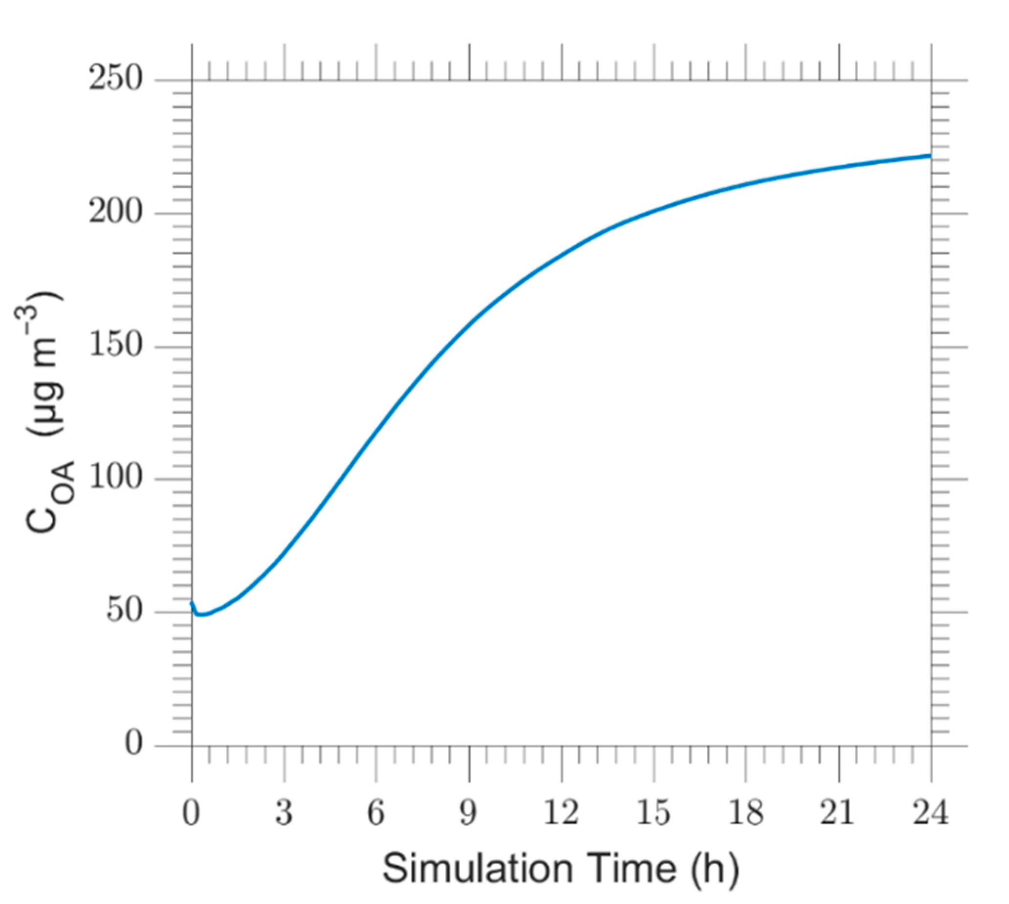
We investigated the evolution of the total organic aerosol concentration included in our column (up to a height of 2.5 km). To do this, we use the average OA concentration inside our column COA, which is given by the equation:
where Hi is the column height (Table S1) and COA,i the organic aerosol concentration of each layer, i. The predicted average OA concentration for the base case is shown in Figure 3. The average OA is predicted to increase by a factor of 4 over the simulated period reaching a steady state.
This evolution implies strong OA production taking place inside the plume for the assumed base case conditions. This increase exceeds most field observations suggesting that the bbSOA parameterization used may be too aggressive.
3.2. Sensitivity Tests
3.2.1. Role of OH Concentration and Aging Rate
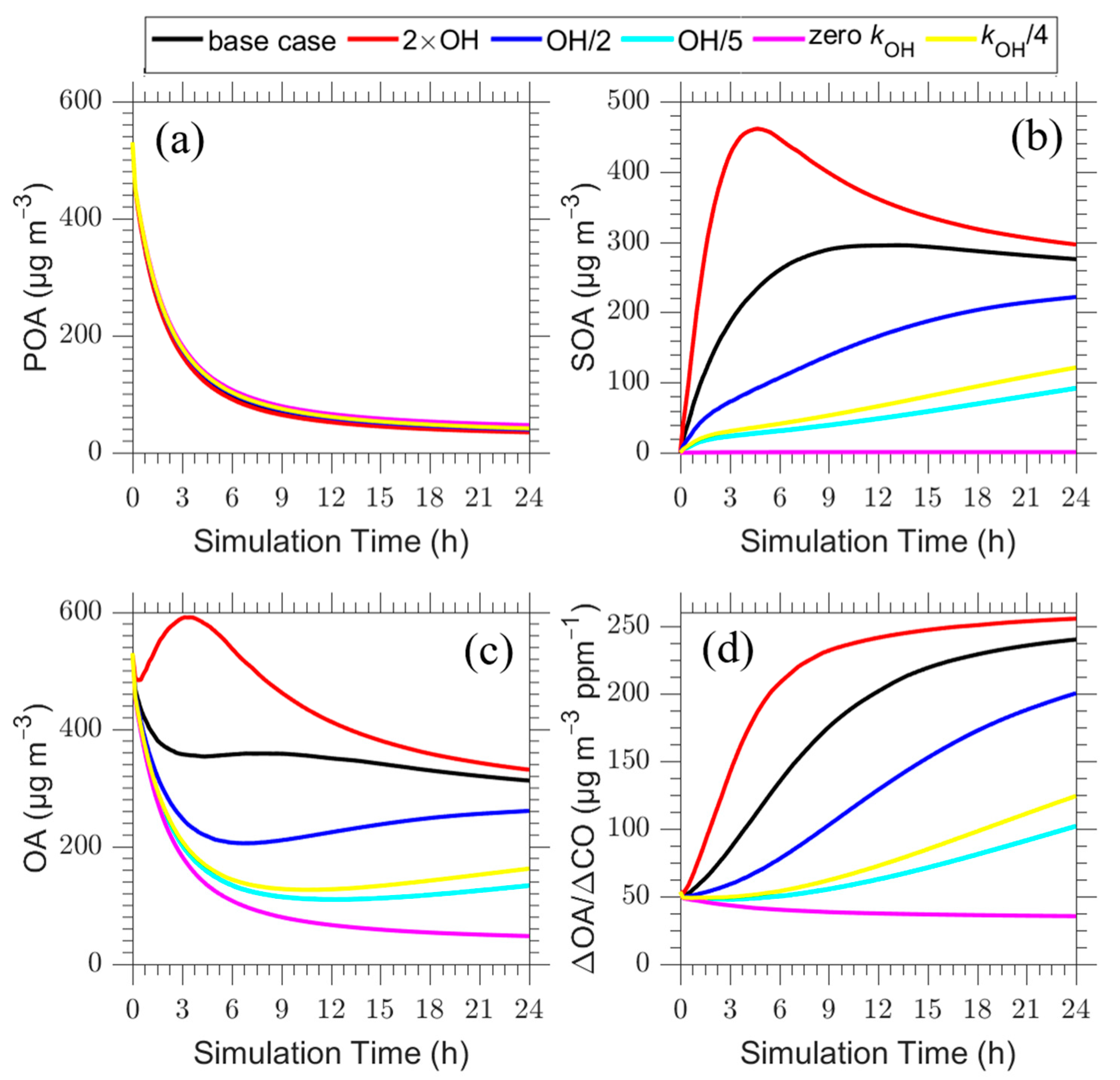
The oxidation of biomass burning plumes is influenced by three key atmospheric oxidants: ozone, the hydroxyl radical, and the nitrate radical. During the day, biomass burning organic compounds are oxidized mainly by ozone and OH, while during the night reactions with the nitrate radical and ozone dominate [35]. The importance of the reactions of the IVOCs and SVOCs with OH, which is the main mechanism of bbSOA formation in PMCAMx-Trj, depends mainly on the OH concentration. In this section, we focus on the effect of the OH concentrations and the daytime evolution and aging of the biomass burning plumes.
As a first test the OH concentration was doubled from its base value of 5 × 10⁶ molecule cm−3 [12] to 1 × 10⁷ molecule cm−3. This higher value corresponds to the OH concentration observed in a biomass burning event in Yokelson et al. [17]. In the second test the OH concentration was decreased by a factor of two to 2.5 × 10⁶ molecule cm−3. In order to further compare our results with the literature we decreased the OH concentration by a factor of five, to 1 × 10⁶ molecule cm−3 which corresponds to the value used by Bian et al. [24]. The aging rate constant remained constant at 4 × 10⁻¹¹ molecule−1 cm3 s−1 which is higher by a factor of eight from the one used by Bian et al. [24]. Finally, to quantify the contribution of SOA chemistry we examined two cases of the aging rate constant. In the first one, the aging rate constant was assumed to be zero and in the second one is decreased by a factor of four (kOH = 1 × 10⁻¹¹ molecule−1 cm3 s−1).
The results of these sensitivity tests for the plume centerline are shown in Figure 4. According to sensitivity tests, the change in both OH and aging rate constant does not significantly change the concentration of POA. The largest change in POA was a 20% increase at the end of the simulation. In contrast, the SOA concentration is highly dependent on OH concentration and aging rate constant.
The increase of OH concentration by a factor of two, resulted in a rapid increase (65%) in ΔOA/ΔCO for the first 5 h (ΔOA/ΔCO = 192 μg m−3 ppm−1 in comparison to 117 μg m−3 ppm−1 of the base case; Figure 4d) due to the fast oxidation rate. After the five hours the production slows down as the system has been depleted of reacting vapors and the ΔOA/ΔCO remains approximately constant. At the end of the 24 h a 6% increase was observed in ΔOA/ΔCO (ΔOA/ΔCO = 255 μg m−3 ppm−1 in comparison to 240 μg m−3 ppm−1 of the base case), indicating a small increase in the final SOA formation. Decreasing the OH concentration by a factor of two resulted in a net decrease of 15% in the final ΔOA/ΔCO (200 μg m−3 ppm−1) and decreasing it by a factor of five resulted in a 60% reduction in ΔOA/ΔCO (100 μg m−3 ppm−1). These indicate that for all these scenarios SOA formation dominates over the evaporation of POA. At the end of the first five hours the predicted increase in ΔOA/ΔCO was 40%, when the OH concentration decreased by a factor of two (ΔOA/ΔCO = 70 μg m−3 ppm−1) and 60% when OH was decreased by a factor of five (ΔOA/ΔCO = 50 μg m−3 ppm−1) due to the corresponding slow SOA formation.
All the OH concentration sensitivity cases lead to an increase in ΔΟΑ/ΔCO by a factor of 2 to 5 compared to the fresh plume (initial condition) after 24 h of photochemical processing at a fixed OH level. The rate of this increase is strongly dependent on the OH level, with the change in ΔΟΑ/ΔCO after 5 h varying from almost zero in the low OH case (one fifth of base case OH), to 40% in the half base case OH scenario, 120% in the base case and 300% in the high-OH case.
If the aging reactions are neglected, ΔΟΑ/ΔCO decreases slowly from 50 μg m−3 ppm−1 to 40 μg m−3 ppm−1 due to POA evaporation (Figure 4d). The results of the scenario in which the aging rate constant is reduced by a factor of four are quite similar to those of the reduction of the OH level by a factor of five. Both of these parameters affect the rate and the conversion of the POA and IVOCs to SOA.
3.2.2. Role of Temperature
In this test, we changed the temperature of the base case (25 °C) to 15 °C, 20 °C, 30 °C and 35 °C in order to investigate its effect on the chemical evolution of the plume. POA evaporation is favored at an increased temperature and therefore the predicted POA decreases as the temperature increases and vice versa. The corresponding results are shown in Figure 5.
The behavior of the predicted SOA is more complicated. An increase in temperature produces less SOA in the first half of the simulation, but the behavior is reversed after that point. In the end of the simulation an increase in temperature is predicted to lead to higher SOA. Increasing temperature favors the partitioning of the SOA to the gas phase leading to lower SOA levels. At the same time the higher temperatures favor the evaporation of the bbPOA and the increase in the SVOC levels and the acceleration of the SOA production. These two effects have opposite directions and for the conditions of this simulation the first dominates in the first half and the latter in the second half of the simulation.
Temperature is predicted to significantly affect the OA in the plume only during its first hours of evolution (Figure 5c) During the first 12 h, there are significant differences in the predicted OA levels, but then the results converge. The OA concentration after 3 h increases by approximately 60% as the temperature decreases from 35 to 15 °C. However, as the plume continues to age, its OA concentration becomes less and less sensitive to temperature and after 24 h, all scenarios have practically the same predicted OA level. The ΔΟΑ/ΔCΟ increases by 12% when temperature drops from 25 to 15 °C and decreases by 15% when temperature increases from 25 to 35 °C in the first 5 h. At the end of the simulation the ΔΟΑ/ΔCΟ is also not dependent on temperature. As a result, temperature in this VBS formulation of the bbOA evolution significantly affects the OA in the plume only during its first hours of evolution, and after that the OA levels are relatively insensitive to this meteorological parameter.
3.2.3. Role of bbOA Volatility Distribution
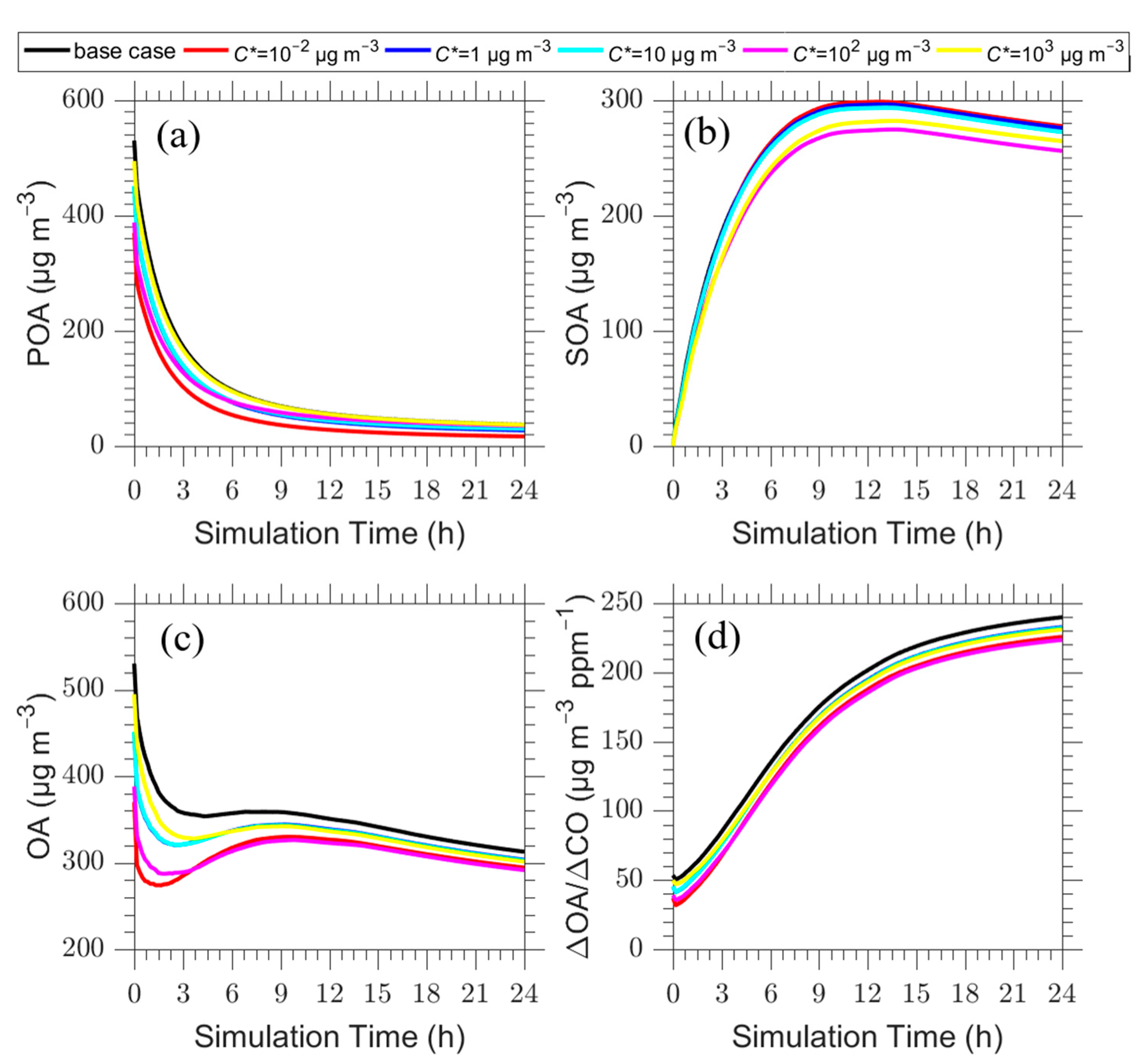
In the base case, the total organic compound emissions of the fire are distributed into eight logarithmically spaced volatility bins based on the volatility distribution of May et al. [36] (Table S2). In this test, we zeroed one at a time the emissions in each volatility bin and repeated the simulation to investigate the role of the emissions in the different volatility ranges in the predicted evolution of the OA in the plume. The corresponding results are shown in Figure 6 and Figure 7.
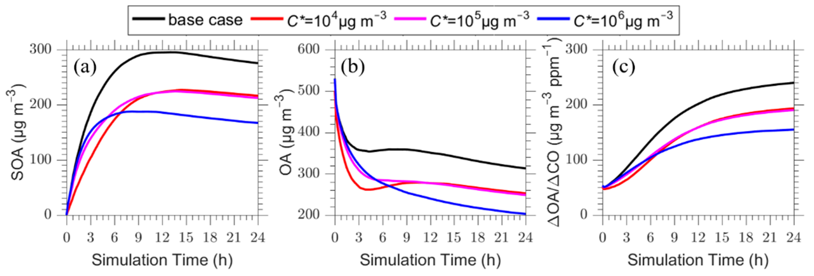
Zeroing the LVOC and SVOC emissions (Ci* = 10−2 to 103 μg m−3 bins) has little effect on the predicted ΔΟΑ/ΔCO. The corresponding change from the base case predictions is less than 6% in the end of the simulation (Figure 6). On the other hand, the IVOC emissions in the 104 to 106 μg m−3 bins even if they are in the gas phase initially play a major role in the predicted OA evolution (Figure 7).
These vapors get oxidized producing SOA that is predicted to dominate the OA behavior after the initial stage of evolution. For example, neglecting the C* = 106 μg m−3 emissions leads to a 35% reduction in ΔOA/ΔCO after 24 h. The IVOCs with C* = 106 μg m−3 contribute the most at long timescales because they are assumed to have the highest emissions and can undergo several generations of oxidation, before their products are transferred to the particulate phase.
3.2.4. Functionalization and Fragmentation
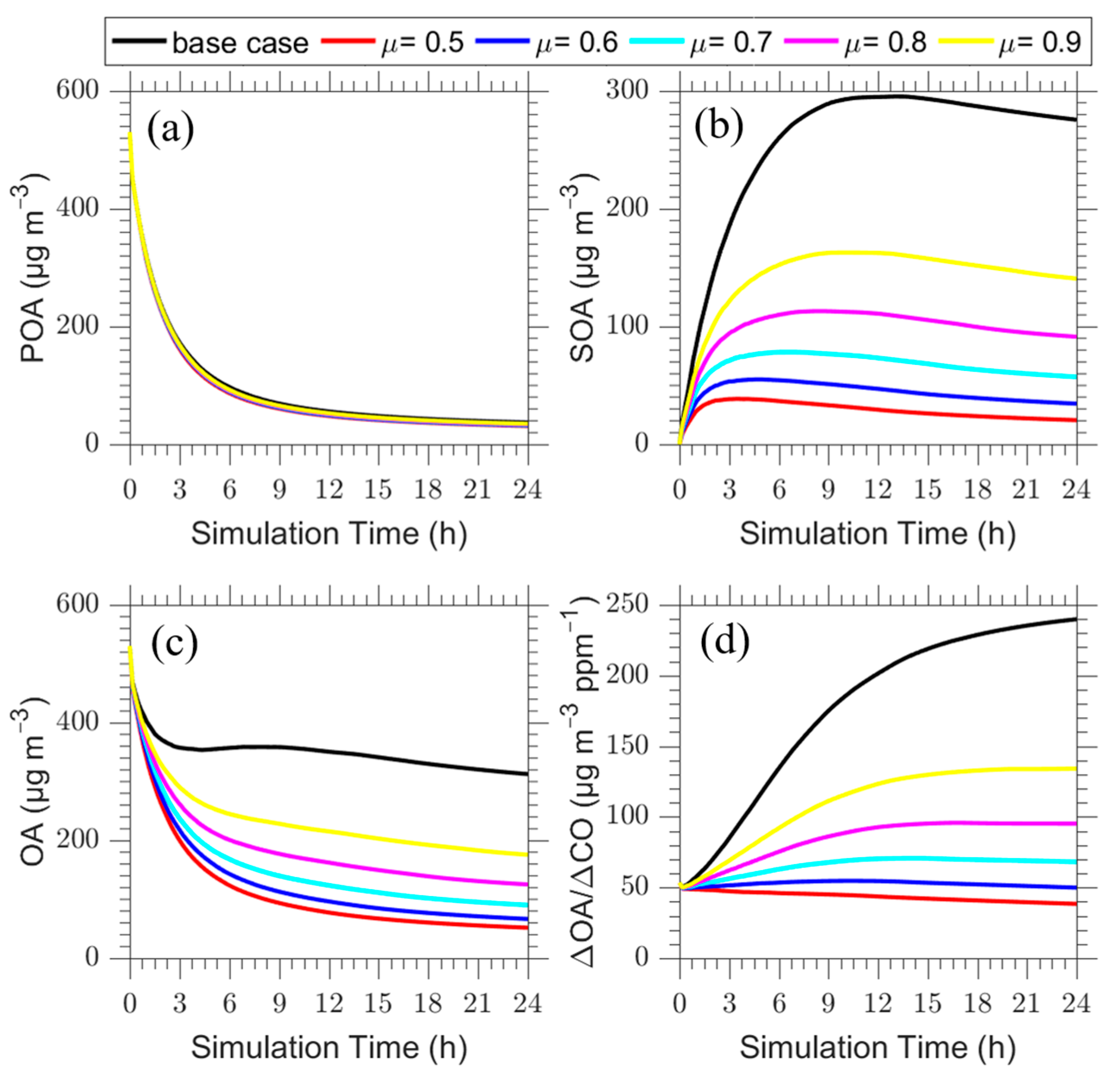
In the base case, functionalization of the organic compounds is assumed to be the only oxidation aging pathway. Each aging reaction step is assumed to reduce the volatility of the reacting vapor by one order of magnitude (i.e., shifting material from C* of 100 to 10 μg m−3), with a small net increase in mass (7.5%) to account for added oxygen. The mass stoichiometric yield (μ) of the aging reactions is assumed therefore to be equal to 1.075. The products of this oxidation (secondary organic vapors) are allowed to partition between the gas and particle phase according to their volatility. This results in the formation of oxidized organic aerosol (referred to as SOA in this work). Intermediate volatility species (IVOC), that are co-emitted with the POA but are never in the particle phase during the emission process, also age in the same way to form SOA.
In this sensitivity test, we decreased μ in all reactions of IVOCs and SVOCs from its base case value of 1.075 to 0.9, 0.8, 0.7, 0.6 and 0.5. The selected values appear to cover most the expected range for the fragmentation probability in these systems [37,38]. These sensitivity tests assume that some organic compounds fragment after reacting with OH leading to products with higher volatility that remain in the gas phase during the rest of the simulation. The corresponding results are shown in Figure 8.
The PMCAMx-Trj predictions for SOA, OA and ΔOA/ΔCO are quite sensitive to the assumed value of the functionalization/fragmentation split. On the other hand, the predicted POA is not that sensitive to the parameterization of the aging pathways. As an example, for the case of μ = 0.8, the predicted SOA decreases by a factor of 3 compared to the base case. This leads to a 60% decrease in ΔΟΑ/ΔCO compared to the base case. ΔΟΑ/ΔCO doubles after a few hours and then remains constant. This behavior is more in-line with the measured evolution of biomass burning plumes in the field. For the μ = 0.5 case, SOA decreases by a factor of 14 over the simulation period, compared to the base case. In this case ΔΟΑ/ΔCO decreases over time indicating that POA evaporation dominates, instead of SOA formation.
3.3. Role of Horizontal Dilution of the Plume
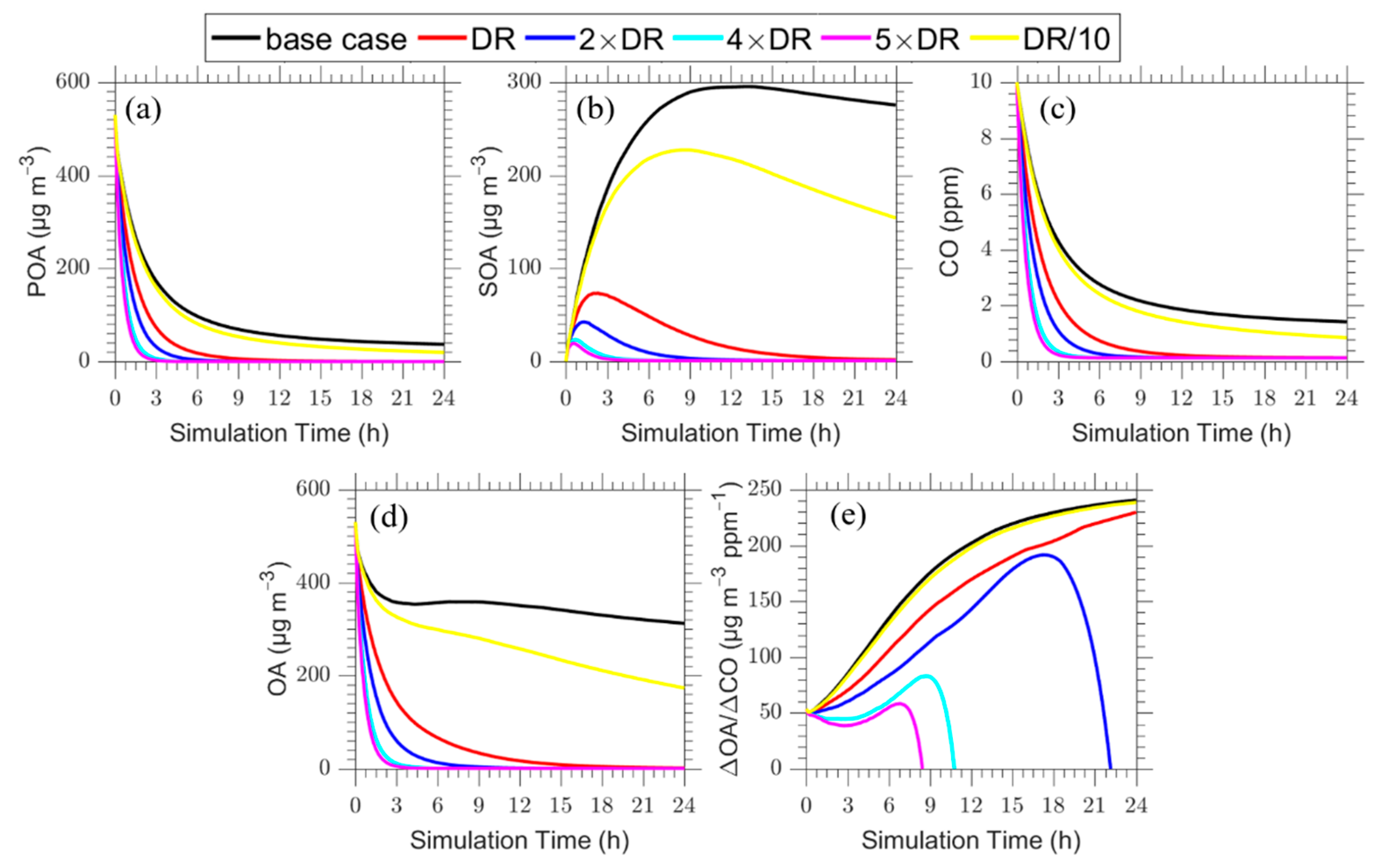
In the base case we assumed that there is no horizontal dispersion, as a result material in the column is not exchanged with the surrounding air. In the first sensitivity test, a horizontal dilution rate constant (DR) k = 10−4 s−1 is assumed together with background concentrations for carbon monoxide [CO]b = 0.13 ppm and [OA]b =1 μg m−3 for organic aerosol. The PMCAMx-Trj predictions for this case are shown in Figure 9. All concentrations decrease faster compared to the base case due to this additional dilution process. The net increase in ΔΟΑ/ΔCO after 5 h of simulation is 75% compared to 120% in the base case. A net increase of 250% is predicted in this case after 15 h compared to ΔΟΑ/ΔCO = 330% for the base case. The predicted absolute concentrations are a lot more sensitive to the horizontal dilution rate than the ΔOA/ΔCO ratio.
In the next series of sensitivity tests, we varied the horizontal dilution rate constant k in the range of 10−5 to 5 × 10⁻⁴ s−1. The corresponding results are summarized in Figure 10. In all cases increasing the horizontal dilution rate leads to decreases of the concentrations of pollutants and more important of the ΔΟΑ/ΔCO. At long enough time scales the plume is diluted enough and the ΔΟΑ/ΔCO approaches that of the background.
These results suggest that the apparent increase in ΔΟΑ/ΔCO is quite sensitive to the assumed horizontal dilution rate constant.
3.3.1. Effect of the Background OA and CO Level
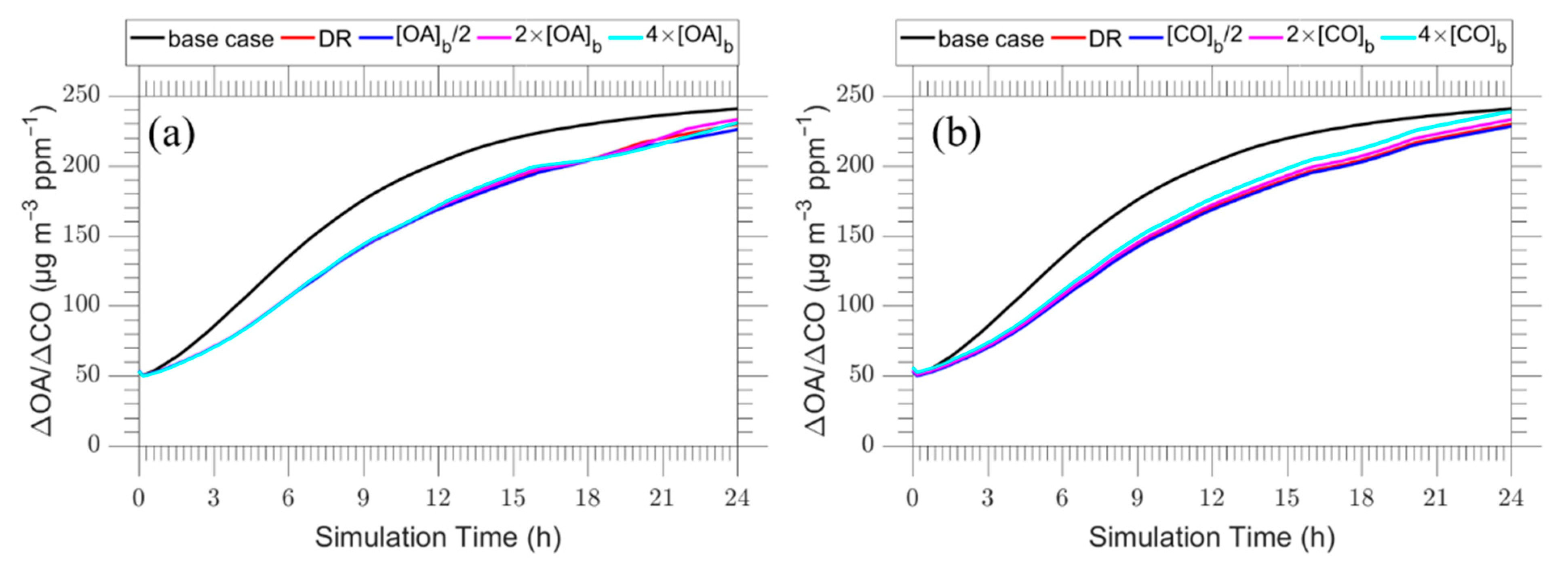
In the first series of sensitivity tests, we investigated the effect of the assumed background OA concentration in the predicted evolution of the plume OA for the dilution case k = 10−4 s−1 discussed in the previous section. The background OA concentration was varied from 0.5 to 4 μg m−3 so that these conditions correspond to a relatively clean background atmosphere. In all cases the background OA concentration was assumed to be highly aged with C* = 10−2 μg m−3 with the corresponding results shown in Figure 11a. The background concentration of organic aerosol has a negligible effect on the evolution of ΔΟΑ/ΔCO for the dilution case. The background concentration needs to be quite high to have a significant effect on the model predictions.
In the next set of simulations, we varied the background concentration of CO which mixes with the fire plume from 0.13 to 0.52 ppm. The corresponding results are shown in Figure 11b. The assumed background concentration of CO has practically no effect on the predicted evolution of ΔΟΑ/ΔCO over the first 5 h. Its effect remains quite small but increases a bit during the second half of the simulation. This is an interesting result, since CO is considered inert in our model, and increases the utility of the ΔOA/ΔCO metric in the analysis of field measurements in similar situations. The OH level is prescribed in our simulations, so it is not affected by changes in the assumed background NOx.
3.3.2. Vertical Dispersion Rate
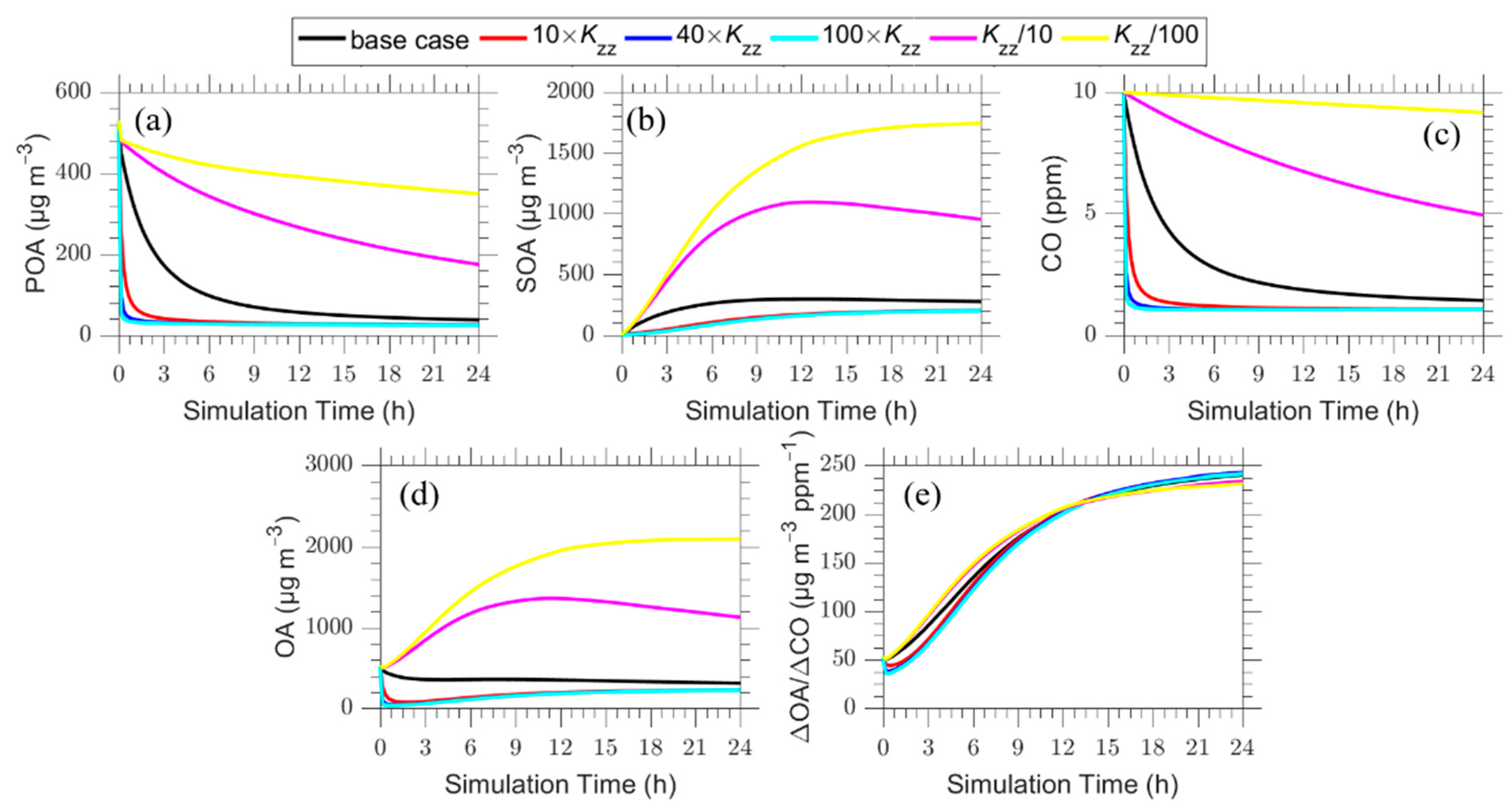
In the base case the assumed vertical turbulent coefficient dispersion (Kzz) was 5 m2 s−1 which corresponds to quite weak vertical mixing. In the sensitivity tests the vertical coefficient dispersion varied over an extreme range of 0.05 (reduction by a factor of 100 from the base case) to 500 m2 s−1 (an increase of a factor of 100). The minimum value of 0.05 m2 s−1 practically means that there is no vertical mixing, while the maximum value of 500 m2 s−1 corresponds to rapid vertical mixing in all layers. The results are shown in Figure 12. As expected, these changes affect dramatically the predicted POA, SOA and CO evolution, with higher vertical dispersion leading to lower concentrations. The surprising result in these simulations is the low sensitivity of the predicted ΔOA/ΔCO to the assumed vertical dispersion coefficient. The increase of the vertical dispersion rate coefficient leads to a decrease of the ΔOA/ΔCO by 20–30% compared to the base case mainly in the first 5 h. The reduction of the vertical dispersion rate increases the ΔOA/ΔCO in the first 8 h, with a maximum increase of approximately 15% appearing at 4 h, for the cases Kzz = 0.5 m2 s−1 and Kzz = 0.05 m2 s−1 while at the end of the 24 h, there is a decrease of −5% in ΔOA/ΔCO.
In our simulations, vertical dispersion is capped at 2.5 km because of the vertical extent of our modeling domain. This limited domain (including of course the effect of the ground) contributes to the different predicted sensitivity of the ΔOA/ΔCO to the horizontal and vertical dispersion. These differences suggest that the estimated sensitivity depends on the approach used for the parameterization of the turbulent dispersion. The oversimplified parcel models that assume that this rate is proportional to the difference of concentrations inside the simulated system and its surroundings appear to be too sensitive compared to the models that simulate more accurately the dispersion process.
4. Conclusions
The one-dimensional Lagrangian version of the CTM PMCAMx (PMCAMx-Trj) was used to simulate the evolution of biomass burning plumes based on the original Volatility Basis Set parameterization of the corresponding aging process. The evolution of the plume is simulated for 24 h of equivalent daytime processing. Nighttime processing is neglected.
Assuming low horizontal dilution, the predicted normalized total bbOA (primary and secondary) increases by a factor of two over the first 5 h which is in agreement with the upper limit of the values observed in some field studies [19,20,21,24]. However, the model predicts that the normalized OA levels continue to increase, with enhancements up to a factor of 4–5 after 24 h of photochemical processing. Such high enhancements have not been observed in the field so far.
Higher oxidant concentrations lead to higher OA concentrations downwind of a fire. The predicted normalized OA (ΔΟΑ/ΔCO) is predicted to increase by a factor of 6 far downwind of a fire as the OH increases from zero to 107 molecule cm−3. Additionally, for the very low photochemical activity levels the normalized OA is predicted to decrease with time, while the opposite happens for modest and high OH levels.
The OH level is prescribed in our simulations, so it is not affected by changes in either the plume or the assumed background NOx. The effect of NOx and may be SO2 (both inside and outside the fire plume) on the biomass burning OA evolution deserves additional attention. These effects have been neglected in the present study in which the gas-phase chemistry has been highly parameterized and can be the topics of future work.
The effects of temperature are different for the various bbOA components and depend on the distance from the fire. POA levels decrease with increasing temperature due to evaporation, while SOA decreases close to the fire and increases further away. Temperature does not seem to explain the low net SOA formation in atmospheric plumes, while it is predicted to affect significantly the OA in the plume, but only during its first hours of evolution. After the first 12 h of simulation the OA levels are relatively insensitive to temperature, because the various effects on the partitioning of POA and SOA and the corresponding aging reactions cancel each other to a large extent. This complexity may explain part of the discrepancies in previous fire plume evolution field studies.
The IVOC emissions dominate the simulated SOA production and therefore the modeled bbOA evolution in longer timescales. The results are also quite sensitive to the assumed functionalization-fragmentation split during the IVOC/SVOC oxidation reactions with OH. These results underline the importance of both the IVOC emissions and their aging chemistry on modeling bbOA and suggest that the representation of aging reactions is more important than the choice of the emitted primary OA volatility distribution for at least the period after a few hours. A functionalization and fragmentation split of 0.8 appears to produce results that are more consistent with available observations compared to the currently used functionalization only approach. Fragmentation of the reacting organic compounds during their oxidation chemistry represents a probable explanation of the low net SOA formation in a number of field studies.
The effects of turbulent dispersion appear to depend on the approach used for the parameterization of the corresponding processes. Assuming that the horizontal dilution rate is simply proportional to the difference in concentrations in the modeled column and its surrounding resulted in significant sensitivity of the normalized OA to the choice of the dilution rate constant, a result similar to previous modeling studies. However, simulating the turbulent dispersion in more detail in the vertical direction resulted in low sensitivity to the corresponding turbulent dispersion coefficient.
In summary, the predicted normalized OA downwind of a fire is sensitive to a number of meteorological and chemical variables. This sensitivity could explain the differences among the various field campaigns and also the differences between laboratory and field studies.
The VBS parameterization with a fragmentation probability around 0.2 will be examined in future studies with the 3-dimensional chemical transport model PMCAMx-SR. This model represents biomass burning emissions and their oxidation products separately from the other OA components and allows the use of any parameterization for this specific source [39]. PMCAMx-SR model will be used to simulate the spatial-temporal dynamics of emissions and atmospheric processing and compare its predictions with aerosol observations.
Supplementary Materials
The following are available online at https://0-www-mdpi-com.brum.beds.ac.uk/article/10.3390/atmos12121638/s1, Table S1: Vertical model structure, Table S2: Volatility distribution of organic compounds emitted by the fire in the base case.
Author Contributions
D.P., E.K. and L.P. carried out the simulations and the analysis, D.P. wrote the final manuscript with support from S.N.P., E.K. and L.P., S.N.P. supervised and coordinated the work. All authors provided critical feedback and helped shape the research, analysis and manuscript. All authors have read and agreed to the published version of the manuscript.
Funding
This work was supported by the project FORCeS funded from the European Union’s Horizon 2020 research and innovation programme under grant agreement No 821205.
Institutional Review Board Statement
Not applicable.
Informed Consent Statement
Not applicable.
Data Availability Statement
The model results used in the present study are available upon request ([email protected]).
Conflicts of Interest
The authors declare no conflict of interest.
References
- WHO. 7 Million Premature Deaths Annually Linked to Air Pollution. 2014. Available online: https://www.who.int/news/item/25-03-2014-7-million-premature-deaths-annually-linked-to-air-pollution/ (accessed on 10 July 2021).
- Lelieveld, J.; Evans, J.S.; Fnais, M.; Giannadaki, D.; Pozzer, A. The contribution of outdoor air pollution sources to premature mortality on a global scale. Nature 2015, 525, 367–371. [Google Scholar] [CrossRef]
- Pope, C.A.; Dockery, D.W. Health effects of fine particulate air pollution: Lines that connect. J. Air Waste Manag. Assoc. 2006, 56, 709–742. [Google Scholar] [CrossRef]
- Haywood, J.; Boucher, O. Estimates of the direct and indirect radiative forcing due to tropospheric aerosols, A review. Rev. Geophys. 2000, 38, 513–543. [Google Scholar] [CrossRef]
- Alonso-Blanco, E.; Calvo, A.I.; Pont, V.; Mallet, M.; Fraile, R.; Castro, A. Impact of biomass burning on aerosol size distribution, aerosol optical properties and associated radiative forcing. Aerosol Air Qual. Res. 2014, 14, 708–724. [Google Scholar] [CrossRef] [Green Version]
- IPCC. Climate Change 2013: The Physical Science Basis: Working Group I Contribution to the Fifth Assessment Report of the Intergovernmental Panel on Climate Change; Cambridge University Press: New York, NY, USA, 2014. [Google Scholar]
- Akagi, S.K.; Yokelson, R.J.; Wiedinmyer, C.; Alvarado, M.J.; Reid, J.S.; Karl, T.; Crounse, J.D.; Wennberg, P.O. Emission factors for open and domestic biomass burning for use in atmospheric models. Atmos. Chem. Phys. 2011, 11, 4039–4072. [Google Scholar] [CrossRef] [Green Version]
- Bond, T.C.; Doherty, S.J.; Fahey, D.W.; Forster, P.M.; Bernsten, T.; DeAngelo, B.J.; Flanner, M.G.; Ghan, S.; Kärcher, B.; Koch, D.; et al. Bounding the role of black carbon in the climate system: A scientific assessment. J. Geophys. Res. 2013, 118, 5380–5552. [Google Scholar] [CrossRef]
- Yokelson, R.J.; Christian, T.J.; Karl, T.G.; Guenther, A. The tropical forest and fire emissions experiment: Laboratory fire measurements and synthesis of campaign data. Atmos. Chem. Phys. 2008, 8, 3509–3527. [Google Scholar] [CrossRef] [Green Version]
- Heilman, W.E.; Liu, Y.; Urbanski, S.; Kovalev, V.; Mickler, R. Wildland fire emissions, carbon, and climate: Plume rise, atmospheric transport, and chemistry processes. For. Ecol. Manag. 2014, 31, 70–79. [Google Scholar] [CrossRef]
- Jolleys, M.D.; Coe, H.; McFiggans, G.; Capes, G.; Allan, J.D.; Crosier, J.; Williams, P.I.; Allen, G.; Bower, K.N.; Jimenez, J.L.; et al. Characterizing the aging of biomass burning organic aerosol by use of mixing ratios: A meta-analysis of four regions. Environ. Sci. Technol. 2012, 46, 13093–13102. [Google Scholar] [CrossRef]
- Akagi, S.K.; Craven, J.S.; Taylor, J.W.; McMeeking, G.R.; Yokelson, R.J.; Burling, I.R.; Urbanski, S.P.; Wold, C.E.; Seinfeld, J.H.; Coe, H.; et al. Evolution of trace gases and particles emitted by a chaparral fire in California. Atmos. Chem. Phys. 2012, 12, 1397–1421. [Google Scholar] [CrossRef] [Green Version]
- May, A.A.; Lee, T.; McMeeking, G.R.; Akagi, S.; Sullivan, A.P.; Urbanski, S.; Yokelson, R.J.; Kreidenweis, S.M. Observations and analysis of organic aerosol evolution in some prescribed fire smoke plumes. Atmos. Chem. Phys. 2015, 15, 6323–6335. [Google Scholar] [CrossRef] [Green Version]
- Cubison, M.J.; Ortega, A.M.; Hayes, P.L.; Farmer, D.K.; Day, D.; Lechner, M.J.; Brune, W.H.; Apel, E.; Diskin, G.S.; Fisher, J.A.; et al. Effects of aging on organic aerosol from open biomass burning smoke in aircraft and laboratory studies. Atmos. Chem. Phys. 2011, 11, 12049–12064. [Google Scholar] [CrossRef] [Green Version]
- Hodshire, A.L.; Akherati, A.; Alvarado, M.J.; Brown-Steiner, B.; Jathar, S.H.; Jimenez, J.L.; Kreidenweis, S.M.; Lonsdale, C.R.; Onasch, T.B.; Ortega, A.M.; et al. Aging effects on biomass burning aerosol mass and composition: A critical review of field and laboratory studies. Environ. Sci. Technol. 2019, 53, 10007–10022. [Google Scholar] [CrossRef]
- Grieshop, A.P.; Logue, J.M.; Donahue, N.M.; Robinson, A.L. Laboratory investigation of photo chemical oxidation of organic aerosol from wood fires 1: Measurement and simulation of organic aerosol evolution. Atmos. Chem. Phys. 2009, 9, 1263–1277. [Google Scholar] [CrossRef] [Green Version]
- Yokelson, R.J.; Crounse, J.D.; DeCarlo, P.F.; Karl, T.; Urbanski, S.; Atlas, E.; Campos, T.; Shinozuka, Y.; Kapustin, V.; Clarke, A.D.; et al. Emissions from biomass burning in the Yucatan. Atmos. Chem. Phys. 2009, 9, 5785–5812. [Google Scholar] [CrossRef] [Green Version]
- Singh, H.B.; Anderson, B.E.; Brune, W.H.; Cai, C.; Cohen, R.C.; Crawford, J.H.; Cubison, M.J.; Czech, E.P.; Emmons, L.; Fuelberg, H.E.; et al. The ARCTAS science team. Pollution influences on atmospheric composition and chemistry at high northern latitudes Boreal and California forest fire emissions. Atmos. Environ. 2010, 44, 4553–4564. [Google Scholar] [CrossRef]
- Konovalov, I.B.; Beekmann, M.; Berezin, E.V.; Formenti, P.; Andreae, M.O. Probing into the aging dynamics of biomass burning aerosol by using satellite measurements of aerosol optical depth and carbon monoxide. Atmos. Chem. Phys. 2017, 17, 4513–4537. [Google Scholar] [CrossRef] [Green Version]
- Vakkari, V.; Kerminen, V.-M.; Beukes, J.P.; Tiitta, P.; van Zyl, P.G.; Josipovic, M.; Venter, A.D.; Jaars, K.; Worsnop, D.R.; Kulmala, M.; et al. Rapid changes in biomass burning aerosols by atmospheric oxidation. Geophys. Res. Lett. 2014, 41, 2644–2651. [Google Scholar] [CrossRef] [Green Version]
- Vakkari, V.; Beukes, J.P.; Dal Maso, M.; Aurela, M.; Josipovic, M.; van Zyl, P.G. Major secondary aerosol formation in southern African open biomass burning plumes. Nat. Geosci. 2018, 11, 580–583. [Google Scholar] [CrossRef]
- Jolleys, M.D.; Coe, H.; McFiggans, G.; Taylor, J.W.; O’Shea, S.J.; Le Breton, M.; Bauguitte, S.J.B.; Moller, S.; Di Carlo, P.; Aruffo, E.; et al. Properties and evolution of biomass burning organic aerosol from Canadian boreal forest fires. Atmos. Chem. Phys. 2015, 15, 3077–3095. [Google Scholar] [CrossRef] [Green Version]
- Alvarado, M.J.; Lonsdale, C.R.; Yokelson, R.J.; Akagi, S.K.; Coe, H.; Craven, J.S.; Fischer, E.V.; McMeeking, G.R.; Seinfeld, J.H.; Soni, T.; et al. Investigating the links between ozone and organic aerosol chemistry in a biomass burning plume from a prescribed fire in California chaparral. Atmos. Chem. Phys. 2015, 15, 6667–6688. [Google Scholar] [CrossRef] [Green Version]
- Donahue, N.M.; Robison, A.L.; Stanier, C.O.; Pandis, S.N. Coupled partitioning, dilution, and chemical aging of semivolatile organics. Environ. Sci. Technol. 2006, 40, 2635–2643. [Google Scholar] [CrossRef]
- Bian, Q.; Jathar, S.H.; Kodros, J.K.; Barsanti, K.C.; Hatch, L.E.; May, A.A.; Kreidenweis, S.M.; Pierce, J.R. Secondary organic aerosol formation in biomass-burning plumes: Theoretical analysis of lab studies and ambient plumes. Atmos. Chem. Phys. 2017, 17, 5459–5475. [Google Scholar] [CrossRef] [Green Version]
- Robinson, A.L.; Grieshop, A.P.; Donahue, N.M.; Hunt, S.W. Updating the conceptual model for fine particulate mass emissions from combustion systems. J. Air Waste Manag. Assoc. 2010, 60, 1204–1222. [Google Scholar] [CrossRef] [PubMed]
- Ford, B.; Val Martin, M.; Zelasky, S.E.; Fischer, E.V.; Anenberg, S.C.; Heald, C.L.; Pierce, J.R. Future fire impacts on smoke concentrations, visibility, and health in the contiguous United States. GeoHealth 2018, 2, 229–247. [Google Scholar] [CrossRef] [Green Version]
- Sakamoto, K.M.; Laing, J.R.; Stevens, R.G.; Jaffe, D.A.; Pierce, J.R. The evolution of biomass-burning aerosol size distributions due to coagulation: Dependence on fire and meteorological details and parameterization. Atmos. Chem. Phys. 2016, 16, 7709–7724. [Google Scholar] [CrossRef] [Green Version]
- Murphy, B.N.; Donahue, N.M.; Fountoukis, C.; Pandis, S.N. Simulating the oxygen content of ambient organic aerosol with the 2D volatility basis set. Atmos. Chem. Phys. 2011, 11, 7859–7873. [Google Scholar] [CrossRef] [Green Version]
- Strader, R.; Lurmann, F.; Pandis, S.N. Evaluation of secondary organic aerosol formation in winter. Atmos. Environ. 1999, 33, 4849–4863. [Google Scholar] [CrossRef]
- Koo, B.Y.; Ansari, A.S.; Pandis, S.N. Integrated approaches to modeling the organic and inorganic atmospheric aerosol components. Atmos. Environ. 2003, 37, 4757–4768. [Google Scholar] [CrossRef]
- Gaydos, T.M.; Pinder, R.; Koo, B.; Fahey, K.M.; Yarwood, G.; Pandis, S.N. Development and application of a three-dimensional aerosol chemical transport model, PMCAMx. Atmos. Environ. 2007, 41, 2594–2611. [Google Scholar] [CrossRef]
- May, A.A.; Levin, E.J.T.; Hennigan, C.J.; Riipinen, I.; Lee, T.; Collett, J.L., Jr.; Jimenez, J.L.; Kreidenweis, S.M.; Robison, A.L. Gas-particle partitioning of primary organic aerosol emissions: 3. Biomass burning. J. Geophys. Res. 2013, 118, 11327–11338. [Google Scholar] [CrossRef]
- Robinson, A.L.; Donahue, N.M.; Shrivastava, M.K.; Weitkamp, E.A.; Sage, A.M.; Grieshop, A.P.; Lane, T.E.; Pierce, J.R.; Pandis, S.N. Rethinking organic aerosols: Semivolatile emissions and photochemical aging. Science 2007, 315, 1259–1262. [Google Scholar] [CrossRef] [PubMed]
- Decker, Z.C.J.; Robinson, M.A.; Barsanti, K.C.; Bourgeois, I.; Coggon, M.M.; DiGangi, J.P.; Diskin, G.S.; Flocke, F.M.; Franchin, A.; Fredrickson, C.D.; et al. Nighttime and daytime dark oxidation chemistry in wildfire plumes: An observation and model analysis of FIREX-AQ aircraft data. Atmos. Chem. Phys. 2021, 21, 16293–16317. [Google Scholar] [CrossRef]
- May, A.A.; McMeeking, G.R.; Lee, T.; Taylor, J.W.; Craven, J.S.; Burling, I.; Sullivan, A.P.; Akagi, S.; Collet, J.L., Jr.; Flynn, M.; et al. Aerosol emissions from prescribed fires in the United States: A synthesis of laboratory and aircraft measurements. J. Geophys. Res. 2014, 119, 11826–11849. [Google Scholar] [CrossRef] [Green Version]
- Donahue, N.M.; Kroll, J.H.; Pandis, S.N.; Robinson, A.L. A two-dimensional volatility basis set—Part 2: Diagnostics of organic-aerosol evolution. Atmos. Chem. Phys. 2012, 12, 615–634. [Google Scholar] [CrossRef] [Green Version]
- Kroll, J.H.; Smith, J.D.; Che, D.L.; Kessler, S.H.; Worsnop, D.R.; Wilson, K.R. Measurement of fragmentation and functionalization pathways in the heterogeneous oxidation of oxidized organic aerosol. Chem. Phys. 2009, 11, 8005–8014. [Google Scholar] [CrossRef] [PubMed] [Green Version]
- Theodoritsi, G.N.; Pandis, S.N. Simulation of the chemical evolution of biomass burning organic aerosol. Atmos. Chem. Phys. 2019, 19, 5403–5415. [Google Scholar] [CrossRef] [Green Version]
Figure 1.
Time dependent vertical profiles of: (a) POA; (b) SOA; (c) total OA; (d) CO concentrations, and (e) ΔOA/ΔCO for the base case.
Figure 1.
Time dependent vertical profiles of: (a) POA; (b) SOA; (c) total OA; (d) CO concentrations, and (e) ΔOA/ΔCO for the base case.

Figure 2.
Time series of (a) organic aerosol concentration; (b) CO concentration; (c) rate difference organic aerosol concentration to the difference of CO concentration at the plume centerline level for the base case. The POA concentration is in black, SOA concentration in blue and the red line is the total OA.

Figure 3.
Time series of the average OA concentration in the simulated air mass.

Figure 4.
Time series of: (a) POA; (b) SOA; (c) total OA; and (d) ΔOA/ΔCO for the plume centerline for the base case (black line) and scenarios of increased OH by a factor of 2 (red line), decreased OH by a factor of 2 (blue line) and a factor of 5 (cyan line), aging rate constant equal to zero (magenta line) or decreased by a factor of four (yellow line).

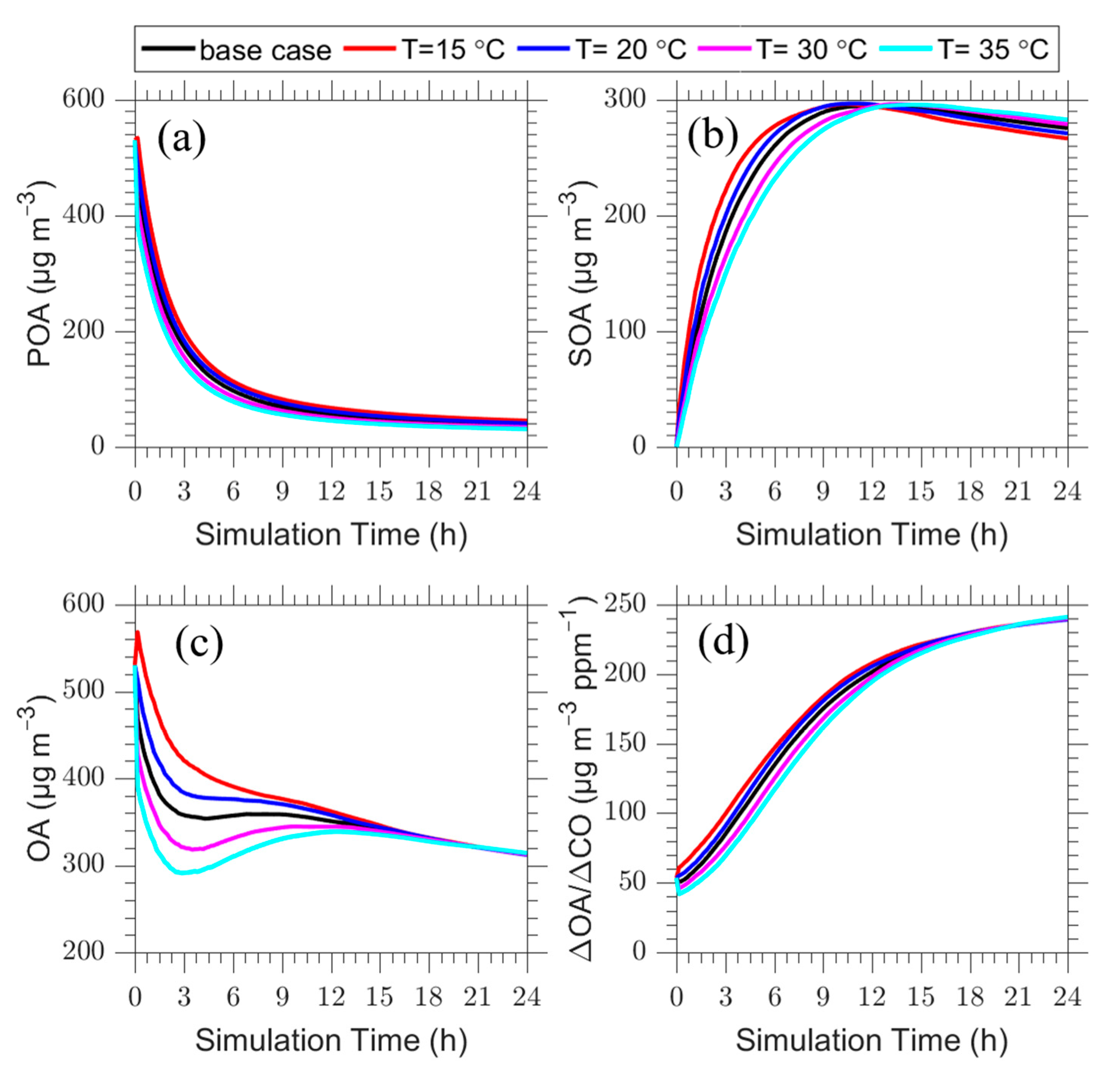
Figure 5.
Time series of: (a) POA; (b) SOA; (c) total OA; and (d) ΔOA/ΔCO for the plume centerline for the base case (T = 25 °C) (black line) and the cases with temperature equal to 15 °C (red line), 20 °C (blue line), 30 °C (magenta line) and 35 °C (cyan line).
Figure 5.
Time series of: (a) POA; (b) SOA; (c) total OA; and (d) ΔOA/ΔCO for the plume centerline for the base case (T = 25 °C) (black line) and the cases with temperature equal to 15 °C (red line), 20 °C (blue line), 30 °C (magenta line) and 35 °C (cyan line).

Figure 6.
Time series of: (a) POA; (b) SOA; (c) total OA; and (d) ΔOA/ΔCO for the plume centerline after zeroing the emissions in the C* =10−2 μg m−3 (red line), 1 μg m−3 (blue line), 10 μg m−3 (cyan line), 102 μg m−3 (magenta line), 103 μg m−3 (yellow line) and the base case (black line).
Figure 6.
Time series of: (a) POA; (b) SOA; (c) total OA; and (d) ΔOA/ΔCO for the plume centerline after zeroing the emissions in the C* =10−2 μg m−3 (red line), 1 μg m−3 (blue line), 10 μg m−3 (cyan line), 102 μg m−3 (magenta line), 103 μg m−3 (yellow line) and the base case (black line).

Figure 7.
Time series of: (a) SOA; (b) total OA; and (c) ΔOA/ΔCO for the plume centerline after zeroing the emissions in the C* = 104 μg m−3 (red line), 105 μg m−3 (magenta line) and 106 μg m−3 (blue line) volatility bins. The base case (black line) is also shown.
Figure 7.
Time series of: (a) SOA; (b) total OA; and (c) ΔOA/ΔCO for the plume centerline after zeroing the emissions in the C* = 104 μg m−3 (red line), 105 μg m−3 (magenta line) and 106 μg m−3 (blue line) volatility bins. The base case (black line) is also shown.

Figure 8.
Time series of (a) POA (in μg m−3), (b) SOA (in μg m−3), (c) total OA (in μg m−3) and (d) ΔOA/ΔCO (in μg m−3 ppm−1) for the seventh layer of the base case (black line) in comparison to the cases with μ = 0.5 (red line), μ = 0.6 (blue line), μ = 0.7 (cyan line), μ = 0.8 (magenta line) and μ = 0.9 (yellow line).

Figure 9.
Time dependent vertical profiles of: (a) POA; (b) SOA; (c) CO; (d) total OA; and (e) ΔOA/ΔCO assuming a horizontal dilution rate constant of k = 10−4 s−1.
Figure 9.
Time dependent vertical profiles of: (a) POA; (b) SOA; (c) CO; (d) total OA; and (e) ΔOA/ΔCO assuming a horizontal dilution rate constant of k = 10−4 s−1.

Figure 10.
Time series of: (a) POA; (b) SOA; (c) CO; (d) total OA; and (e) ΔOA/ΔCO for the plume centerline for the base case (black line) in comparison to the cases with dilution rate constants DR equal to 10−4 s−1 (red line), and increased dilution rate by a factor of 2 (blue line), 4 (cyan line) and 5 (magenta line) and decreased dilution rate by a factor of 10 (yellow line).

Figure 11.
Time series of ΔOA/ΔCO for the plume centerline for the: (a) increased background OA cases by a factor of 2 (magenta line) and 4 (cyan line) and decreased background OA case by a factor of 2 (blue line) and (b) increased background CO cases by a factor of 2 (magenta line) and 4 (cyan line) and decreased background CO cases by a factor of 2 (blue line). The base dilution case (red line) and overall base case (black line) are also shown.

Figure 12.
Time series of: (a) POA; (b) SOA; (c) CO; (d) total OA; and (e) ΔOA/ΔCO for the plume centerline for the base case (Kzz = 5 m2 s−1) (black line) and the sensitivity cases with vertical dispersion Kzz = 50 m2 s−1 (red line), 200 m2 s−1 (blue line), 500 m2 s−1 (cyan line), 0.5 m2 s−1 (magenta line) and 0.05 m2 s−1 (yellow line).


Table 1.
Conditions and plume parameters for the base case.
| Condition | Value |
|---|---|
| OH concentration (molecule cm−3) | 5 × 10⁶ |
| Horizontal dilution rate constant (s−1) | 0 |
| Aging rate constant (kOH, cm3 molecule−1 s−1) | 4 × 10⁻¹¹ |
| Vertical dispersion coefficient (Kzz, m2 s−1) | 5 |
| Plume injection layer | 750–1000 m |
| Temperature (K) | 298 |
| Relative humidity (%) | 50 |
| Pressure (mbar) | 1013.25 |
| Wind speed (m s−1) | 2 |
| Photolysis rate (min−1) | 0.4 |
| Land use type for surface roughness | Deciduous forest |
| Gases | Initial Plume Concentration | Background Concentration |
|---|---|---|
| Carbon monoxide (ppm) | 10 | 0.129 |
| Nitric oxide (ppb) | 0.02 | 0.02 |
| Nitrogen dioxide (ppb) | 0.04 | 0.04 |
| Ozone (ppb) | 50 | 50 |
| Sulfur dioxide (ppb) | 0.12 | 0.12 |
| Nitric acid (ppb) | 0.41 | 0.41 |
| Ammonia (ppb) | 10 | 10 |
| Aerosol components | ||
| Black carbon (μg m−3) | 187 | 0.35 |
| Chloride (μg m−3) | 12 | 0 |
| Ammonium (μg m−3) | 14 | 1.3 |
| Nitrate (μg m−3) | 30 | 0.2 |
| Sulfate (μg m−3) | 0.8 | 6.6 |
Publisher’s Note: MDPI stays neutral with regard to jurisdictional claims in published maps and institutional affiliations. |
© 2021 by the authors. Licensee MDPI, Basel, Switzerland. This article is an open access article distributed under the terms and conditions of the Creative Commons Attribution (CC BY) license (https://creativecommons.org/licenses/by/4.0/).
Share and Cite
MDPI and ACS Style
Patoulias, D.; Kallitsis, E.; Posner, L.; Pandis, S.N. Modeling Biomass Burning Organic Aerosol Atmospheric Evolution and Chemical Aging. Atmosphere 2021, 12, 1638. https://0-doi-org.brum.beds.ac.uk/10.3390/atmos12121638
AMA Style
Patoulias D, Kallitsis E, Posner L, Pandis SN. Modeling Biomass Burning Organic Aerosol Atmospheric Evolution and Chemical Aging. Atmosphere. 2021; 12(12):1638. https://0-doi-org.brum.beds.ac.uk/10.3390/atmos12121638
Chicago/Turabian StylePatoulias, David, Evangelos Kallitsis, Laura Posner, and Spyros N. Pandis. 2021. "Modeling Biomass Burning Organic Aerosol Atmospheric Evolution and Chemical Aging" Atmosphere 12, no. 12: 1638. https://0-doi-org.brum.beds.ac.uk/10.3390/atmos12121638
Note that from the first issue of 2016, this journal uses article numbers instead of page numbers. See further details here.