
Low-Cost Air Quality Sensing towards Smart Homes
by
 , ,
, ,
Hamid Omidvarborna
1 ,
,
Prashant Kumar
1,2,* ,
,
Joe Hayward
1,
Manik Gupta
3 and
Erick Giovani Sperandio Nascimento
4 1
Global Centre for Clean Air Research (GCARE), Department of Civil and Environmental Engineering, Faculty of Engineering and Physical Sciences, University of Surrey, Guildford GU2 7XH, UK
2
Department of Civil, Structural & Environmental Engineering, Trinity College Dublin, D02 PN40 Dublin, Ireland
3
Computer Science and Information Systems, BITS Pilani-Hyderabad Campus, Pilani 500078, India
4
Post-Graduate Program on Computational Modelling and Industrial Technology, SENAI CIMATEC University Centre, 41650-010 Salvador, BA, Brazil
*
Author to whom correspondence should be addressed.
Atmosphere 2021, 12(4), 453; https://0-doi-org.brum.beds.ac.uk/10.3390/atmos12040453
Submission received: 2 March 2021
/
Revised: 21 March 2021
/
Accepted: 29 March 2021
/
Published: 2 April 2021
(This article belongs to the Special Issue The Potential Use of Low-Cost Air Pollution Sensors in Variety of Indoor and Outdoor Applications)
Abstract
:The evolution of low-cost sensors (LCSs) has made the spatio-temporal mapping of indoor air quality (IAQ) possible in real-time but the availability of a diverse set of LCSs make their selection challenging. Converting individual sensors into a sensing network requires the knowledge of diverse research disciplines, which we aim to bring together by making IAQ an advanced feature of smart homes. The aim of this review is to discuss the advanced home automation technologies for the monitoring and control of IAQ through networked air pollution LCSs. The key steps that can allow transforming conventional homes into smart homes are sensor selection, deployment strategies, data processing, and development of predictive models. A detailed synthesis of air pollution LCSs allowed us to summarise their advantages and drawbacks for spatio-temporal mapping of IAQ. We concluded that the performance evaluation of LCSs under controlled laboratory conditions prior to deployment is recommended for quality assurance/control (QA/QC), however, routine calibration or implementing statistical techniques during operational times, especially during long-term monitoring, is required for a network of sensors. The deployment height of sensors could vary purposefully as per location and exposure height of the occupants inside home environments for a spatio-temporal mapping. Appropriate data processing tools are needed to handle a huge amount of multivariate data to automate pre-/post-processing tasks, leading to more scalable, reliable and adaptable solutions. The review also showed the potential of using machine learning technique for predicting spatio-temporal IAQ in LCS networked-systems.
1. Introduction
Indoor air pollution is placed among the top five environmental public health risks that cause morbidity and mortality globally. The majority of people spend more than 90% of their time in indoor environments [1,2], and health problems and diseases associated with poor indoor air quality (IAQ) can cause a variety of adverse health effects to them [3,4]. The time spent indoors recently increased significantly in year 2020 due to severe acute respiratory syndrome coronavirus 2 (SARS-CoV-2) pandemic when people are advised to ‘stay home stay safe’ to protect health workers [5,6].
Table 1 summarises common indoor air pollutants, their sources, and current guidelines to maintain IAQ. Air pollutants inside indoor environments can be generated from different sources, including occupants’ exhalation (carbon dioxide; CO2), activities such as cooking and smoking, emissions from building materials, etc. from which various air pollutants, such as carbon monoxide (CO), particulate matter (PM), and volatile organic compounds (VOCs) are released [2,7]. CO2 is not counted as an air pollutant, but its level represents the performance of ventilation systems, especially in wintertime, whereas high CO2 levels represent poor ventilation and possible accumulation of other indoor air pollutants [8,9,10]. Additionally, IAQ could be affected by local outdoor air pollutants, which can ingress into indoor environments (see Table 1).
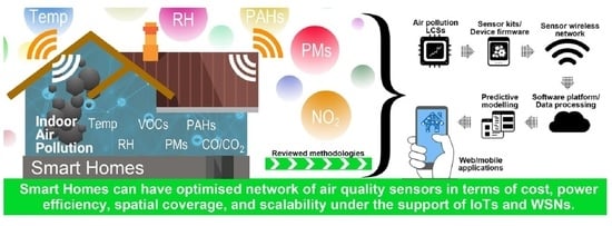
Rapid developments in low-cost sensors (LCSs) and wireless communication technologies have become much more prominent in in everyday life [9,18,19,20,21,22]. LCSs have the potential to revolutionise insufficient IAQ monitoring systems with the prospect of delivering real-time air pollution data through sensor networks, which complement the established reference measurement methods defined in the EU Air Quality Directives (e.g., 2008/50/EC). Although there is no officially agreed definition of the term “low-cost” [23], “low-cost” has been identified by the United States Environmental Protection Agency (US EPA) as devices costing less than $2500 (USD); this is the limit often defining capital investment limits by LCS users [24]. Due to the importance of this technology in the future development of smart homes, the EU has invested millions of Euros on a number of sensor-based projects such as EuNetAir, IAQSense, and SENSIndoor and the similar investments can be seen elsewhere (e.g., USA, Australia). Smart homes can enable an adaptable living environment, e.g., in managing IAQ, to promote comfort and convenience to the occupants. The outcomes of these projects could contribute in the development of novel sensor systems, real-time air pollution monitors, air quality models, and standardised methods [25,26,27,28]. These projects have encouraged research institutions and businesses to take a greater interest in the advancements of sensing technology in IAQ-related research inside smart homes. In the subsequent text, we have interchangeably used the terms “sensor”, “sensor kit” and “LCS”.
Deploying a network of air pollution LCSs with the support of advanced communication technologies is sufficient to provide accurate information in understanding the spatio-temporal distribution of indoor air pollutants and assessment of personal exposures in smart homes. However, among the limited studies focused on LCS applications in indoor environments, studies mainly focused on general applications, benefits/challenges, future demands/directions of LCSs for specific indoor applications [11,23,29,30]. Moreover, their focus on data analysis was limited to changes in concentrations and no prediction or precautionary actions against the possible events were incorporated [31,32]. Although these studies presented promising results, their scope was not to consider the needs of smart homes. Given the scattered information and research gaps in the existing body of literature, this review aims to fill this knowledge gap by summarising the relevant knowledge in different research disciplines, synthesising the emerging themes and providing unique insights for making homes smart with respect to air quality. In particular, the specific objectives of this review are to (i) provide a comprehensive summary of common indoor air pollutants and pros/cons of LCSs manufactured for indoor applications, (ii) review and summarise the optimal deployment strategies of LCSs within a domestic context, (iii) discuss pre-/post-processing protocols to conduct reliable measurements, carry out data management and data processing, and generate useful information for occupants from the large datasets obtained by networked structures, (iv) evaluate the effectiveness of predictive modelling tools to obtain best-fit approaches with an adequate spatial resolution for estimating exposure to indoor air pollution using LCSs.
2. Scope and Outline
The scope of this review is limited to advanced automation technologies, including sensor selection, deployment strategies, data processing, and development of predictive models, which brings healthier indoor environments via monitoring and control of IAQ through the use of networked LCSs. Therefore, a discussion on how to improve IAQ for healthier environments, as well as considerations of ventilation settings, optimal selection of filtration units or air purifying systems are excluded from the scope of this study.
We searched peer-reviewed research articles focusing on the main keywords in various scientific electronic resources, such as Web of Science, ScienceDirect, Wiley, Springer, PubMed and those known to authors. The terminologies used in the search were either one or a combination of “smart homes”, “home automation”, “low-cost sensors”, “affordable pollution sensing”, “sensor deployment strategies”, “data collection”, “data assimilation”, “data processing”, “machine learning”, “data modelling”, “predictive modelling”, “indoor air pollution” and “indoor air quality”. Documents published in the technical reports or the following websites, WHO, UK Department for Environment, Food and Rural Affairs (DEFRA), European Commission, US EPA organisations, and different sensor manufacturers were also reviewed for their contents. Since the topic is broad and explored by private companies/organisations as well, studies/reports outside the aforementioned databases were reviewed as a part of a grey literature review using similar keywords through the Google search engine. Studies that did not have one of the quoted terms or explicitly focused on outdoor/ambient environments were discarded from the analysis. The resulting documents were manually screened and collected information fitting to the context was selected for discussion. The search was limited to English-based articles/reports.
As summarised in Figure 1, the article starts with a brief review of the common indoor air pollutants for developing the background context for the topic areas covered (Section 3), followed by the state-of-the-art air pollution sensing technologies for indoor environments by considering their performance and drawbacks (Section 4). The subsequent section (Section 5) explores optimal deployment strategies to better capture spatio-temporal distribution of indoor air pollutants and addresses how these strategies could be built to improve the accuracy and reliability of data. Section 6 summarises pre- and post-processing methods and tools in dealing with LCSs data. Section 7 describes suitability of advanced IAQ predictive models for indoor settings. Finally, a summary of topic areas covered, conclusions and future remarks are presented in Section 8.
3. Common Indoor Air Pollutants and Their Sources
IAQ is affected by diverse ranges of indoor sources as well as infiltration of outdoor air pollutants. Each source could impact the overall IAQ, depending on their intensity and the operational time (see Table 1). The most common indoor air pollutants arising from indoor occupants, activities and/or materials are CO2, CO, VOCs, and PM in different aerodynamic size fractions, including PM ≤ 2.5µm (PM2.5) and ≤10µm (PM10). Although there can be other pollutants, such as polycyclic aromatic hydrocarbons (PAHs; specifically, benzo[a]pyrene), nitrogen oxides (NOx = NO+NO2), ozone (O3), sulphur dioxide (SO2), formaldehyde (HCHO), radon and persistent organic pollutants (POPs), the presence of all of these components in one place is unlikely. In addition, under-controlled thermal comfort parameters, such as temperature, air velocity, relative humidity (RH), noise and lighting levels are other parameters that make the living environment pleasant for the occupants. Hence, a flow of clean air throughout a building environment is necessary to minimise the risk of accumulation of indoor air pollutants.
4. Sensor Technology
Assessing the existing IAQ and unexpected changes in its level through continuous measurement is necessary to know the status of IAQ and its effects on the occupants’ health. Sensing IAQ with the help of LCSs could be served as the core of smart homes and counted as one of the major components to maintain high-quality living standards. The desirable sensors in smart homes should: (i) be sensitive and selective to target pollutants for reliable sensing relevant to indoor environments that pose health risks to occupants; (ii) be durable with optimal performance over a long-term of deployment; (iii) be small in size, maintenance-free with low-power consumption; (iv) be adopted in complex sensor networks; and (v) work quietly with minimum operating noise [11,12,33,34,35,36,37]. These features enable air pollution sensors to be deployed with relative ease to locations where understanding air quality level could have a huge impact on human health. However, LCSs come with challenges, which may reduce user trust, accuracy and interpretability of recorded data [12,38]. If their quality remained unchanged under realistic conditions, they could become a game-changer in various IAQ measurements [39].
4.1. Electrochemical Sensors
Electrochemical technology is one of the oldest and perhaps widely used technologies for concentration measurements of gaseous pollutants using either potentiometric (measuring a difference of potentials) or amperometric (measuring current of a redox reaction) principles. Fundamentally, electrochemical sensors (ECs) require at least two electrodes (reference and counter electrodes) for operation, which operate based on a chemical reaction between a gaseous pollutant in the air and an electrode in an electrolyte. The sensors are coated with a catalyst that provides a high surface area, which promotes reactions [34]. The recent ECs contain a cell with three electrodes including, measuring, reference and counter electrodes, which host reduction/oxidation of chosen gases. In this technology, the sample gas diffuses through the sensor’s membranes towards the measuring electrode, which results in an electron transfer (produce an internal current). Recently, some sensor manufacturers (e.g., those of AlphaSense and Membrapor, Wallisellen, Switzerland) have upgraded ECs by adding the fourth electrode to monitor physical changes and measure drift [40].
ECs have a comparatively low-cost, high sensitivity/low cross-sensitivity, low detection limit (~sub-ppm), reasonable response time, and less power-intensive (µW) characteristics compared to traditional monitors [34]. Additionally, stability with acceptable drift values (between 2% and 15% per year) have been reported for the commercial ECs (e.g., Nemoto and SGX Sensortech) [40]. However, they are more complicated, vulnerable to poisoning, large in size, of shorter life span (~1–3 years), and more expensive than that of metal oxide semiconductor (MOx) gas sensors (see Section 4.2). As listed in Table 2, ECs have shown interference with the change in meteorology (e.g., air temperature), which is in the first-order impact on an electric output signal of gas concentration (ppb level) and second-order error on gas sensitivity. Low temperatures decrease the speed of reaction in electrochemical cells, which reduce the applicability to operate under cold environments (<10 °C). However, there is a solution to overcome the effects of temperature on background currents (zero currents) that would make a significant impact on measurements at low concentration levels [41].
4.2. Metal Oxide Semiconductor (MOx) Sensors
In MOx sensors, gaseous air pollutants react with the sensor surface and change it’s electrical (resistance or conductivity) properties [44,45]. Measuring the changes in electrical properties represent the concentration of the target pollutant in the air. Because of advances in fabrication methods and the simplicity of semiconductor sensor devices, MOx gas sensors are moderately low-priced compared to other technologies (cheaper than ECs). MOx sensors are robust, lightweight/long-lasting, sensitive to low-concentration gases (as low as ppb level), and less power intensive (less than 1 W) but higher than PIDs (photoionisation detectors; see Section 4.3) [46,47,48].
Simple and fast production processes on a large scale as well as simply controllable processes make MOx gas sensors a desirable technology for air quality monitoring. MOx gas sensors have been reported to be sensitive to a variety of air pollutants [48], with responses changing with the concentration of gaseous pollutants and device operating temperature [46]. MOx gas sensors have been implemented to measure/monitor trace amounts of gaseous pollutants, such as CO, CO2, O3, total VOCs, Ammonia (NH3) and NOx [46,49]. However, non-linear output signals, cross-sensitivity to other gases (especially to changes in environmental conditions and other VOC substances in complex mixtures), poisoned by certain or high doses of target gases (e.g., high concentration of certain organic compounds and gaseous sulphur-containing substances) have been discussed in the literature [12,48,50,51].
4.3. Photoionisation Detectors (PIDs)
The PID is another type of LCS, which uses high-energy photons (ultraviolet (UV) light) for ionisation of gaseous molecules [40]. The main principle is that the gas between the electrodes is ionized by UV light (in the energy scale of 10 eV) to produce charged ions. The resulting ions are proportional to the output signals as well as pollutant concentrations in the detector. Due to high sensitivity, PIDs are extensively used for the detection of VOCs, because each VOC component has its own ionisation potential (IP). IP range varies from easy to ionise substances (~7 eV) to extremely difficult to ionise substances (~12–16 eV). For example, PIDs effectively detect most hazardous gases, including VOCs (e.g., benzene = 9.25; hexane = 10.13; toluene = 8.82; and xylene = 8.56 eV) due to their low IPs, and offer a range of benefits, such as fast response, small size, ease of use/maintenance, and ability to detect low concentrations. However, PIDs cannot detect air constituents (O2 and N2), CO2, CO, SO2, CH4, and O3 due to their high IPs.
4.4. Optical Sensors
Optical sensors, also called light scattering sensors, are used for detection of PMs. Light-scattering PM sensors measure the optical properties of the particles as an ensemble, which offers fast and real-time responses, minimal drift and greatly reduces the cost and size of the sensors [52,53,54,55]. In addition to small size, low-energy consumption (less power supply voltage ~5 V) and ability to generate high-frequency output data during operations make optical sensors a good candidate in various applications [56,57]. Furthermore, variations in PM2.5 concentration measurement under low-concentrations (20–30 μg m−3) among different optical PM sensors against reference instruments could be a major drawback of sensors of this type. This is because the amount of scattered light is reliant on size, shape, density, and refractive index of particles [58]. Despite all these limitations, reliable functioning of optical PM sensors in indoor environments with small spatial scale was reported [59].
4.5. Sensor Selection
Putting multiple sensors together onto boards, calibrating and reshaping them as commercial products for indoor (or outdoor) applications has been a common practice. Such sensor-based products are becoming increasingly available, while the information around lifetime and maintenance are not clearly available. Table 2 (sensors) and Table 3 (commercial sensor-based products) summarise the specification of technologies in the market, whose performances have been evaluated by at least one indoor study. Moreover, the manufacturer’s specifications obtained from technical datasheets, such as type of pollutant, technology, measuring range, reported sensor lifetime, sampling mechanism, sampling interval, environmental operating range, and connectivity have been summarised in Table 3.
Studies showed that the sensor correlations against the research-grade instruments could vary before and/or after deployment even for identical sensors under identical conditions [60,61,62,63]. Furthermore, environmental conditions (temperature and RH) and cross-sensitivities of certain pollutants (e.g., NO2 gas on O3 sensors, NO gas on NO2 sensors, and hydrogen molecule on CO sensors) on sensor readings have been imperfectly addressed [34,38,64,65,66]. In other words, due to the lack of regulatory bodies, questions are raised about their reported values, reproducibility and comparability. However, significant progress has been made in this direction in the recent past. For example, the Air Quality Sensor Performance Evaluation Centre (AQ-SPEC) operated by South Coast Air Quality Management District (SCAQMD) [67,68], the US EPA, Air Sensor Toolbox [69], and the EU Joint Research Centre (EU JRC) [50,70] programs have been initiated to quantitatively evaluate the performance, stability and quality assurance/control (QA/QC) of sensor-based products. To tackle these issues in a more convenient way by not only considering in-field co-location, field normalisation or field calibration with reference instruments [71,72,73], recent studies have shown an alternative solution that can be utilised to improve the QA/QC of readings. Affordable laboratory facilities, such as the Envilution® chamber are currently offered by academic and research institutions to calibrate and evaluate the performance of LCSs before and after deployment under controlled environments [73]. Here, a controlled environment is defined as a situation where changes in environmental conditions and pollution concentrations, representing indoor environments, for testing LCSs can be simulated (controlled) inside the chamber. Therefore, LCSs performance can be assessed under a combination of indoor variations in environmental parameters and pollution concentrations. In-field co-location would be an alternative QA/QC measure after deployment. Moreover, routine calibration checks after deployment for simple networks along with advanced statistical techniques, e.g., data consistency checks, network correlations, and principal components analysis, in complex networks (Section 7) can boost the performance of this system to maintain long-term satisfactory performance. Such platforms, initiatives and programs offer support to obtain reliable data by the use of appropriate sensors, which could result in improving personal exposure estimates in home environments.
5. Deployment Strategies
Enclosed environments such as homes trap more polluted air than open environments due to the presence of indoor sources, lack of free-flow air circulation and inadequate ventilation. In addition, different exposure levels to indoor air pollutants have been reported for individuals even at the same location [32,74]. Unfortunately, the use of conventional monitoring devices are unable to satisfactorily capture a spatial variation and map instantaneous changes in IAQ because of the associated cost, non-scalability, and lack of spatio-temporal mapping of indoor air pollutants [11,30,75,76]. Considering these potentials and demands for technologies, the emergence of LCSs has changed the landscape of IAQ monitoring systems, where specific sensors and sensor-based products are manufactured and designed for indoor applications (see Table 2 and Table 3, respectively). Although air pollution sensors have some drawbacks (Table 2), relatively smaller changes in the environmental parameters and less complexity of indoor air flow patterns compared to outdoor environments could be beneficial for using them indoors. Table 4 summarises examples of the sensor applications in indoor environments, in which less attention has been given to strategies for spatio-temporal distribution of multiple air pollutants. The objectives of the reviewed studies were limited to the performance evaluation of sensors in enclosed environments, in which near-source air pollution monitoring systems or considering an adult’s breathing height as a common practice among the studies is inadequate to assess overall IAQ [35,77,78,79]. Considering indoor arrangements and the relationship between indoor-outdoor environments [80], here we focus our efforts in developing suitable strategies for indoor environments, while air pollution sensors are playing the major role in covering the area.
Air quality sensors should be deployed systematically across a location in order to (i) optimise the cost and the number of sensors according to building layout, space and room features, (ii) ensure the reliability level of the sensor network in case of sensor failure, (iii) provide acceptable spatial and temporal coverage of indoor air pollutants, and (iv) minimise the cost associated to computational analysis and prediction models [23,90,91,92]. There are common suggestions regarding deployment strategies in practical engineering applications, such as sensor selection as per common indoor sources, considering the impacts of outdoor air pollution on indoors, and deploying sensors along the wall with proper accessibility for calibration or maintenance [35,93]. However, sensor deployment strategies, especially for IAQ applications are usually determined based on objective functions and sensor applications [90,94]. In general, deployment strategies in indoor environments vary with time and space, which can be categorised into (i) engineering, and (ii) optimisation methods. In the engineering method, previous experiences and rules of thumb are incorporated. Uniform deployment of several sensors in space would be a common practice in engineering methods as can be seen in studies listed in Table 4, which may result in a fairly expensive and unfeasible output in some cases. Application of this method may result in lack of (i) spatio-temporal mapping, (ii) controlling the response time, and (iii) generalisability to multiple rooms/spaces [90,94,95]. To compensate for the limitations of this method, the optimisation method has recently developed, in which indoor airflow patterns in the deployment of sensors are taken into account [96,97,98,99,100]. In this method, modelling tools such as computational fluid dynamics (CFD), zonal model, and multi-zone airflow model are utilised along with genetic algorithm, artificial neural networks (ANNs), simulated annealing, and stochastic approximation methods to optimise objective, cost, or fitness functions based on the predefined goals [97,98,101,102]. Although this method could bring precision in choosing the optimal strategy, optimisation methods could be computationally intensive in the large deployment of sensors in multi-zone airflow and CFD-based simulations [95]. Nevertheless, to achieve optimal strategies regardless of sensor locations and to avoid occasional error in the prediction results of small sensor networks (a combination of 3 to 4 sensors as reported by Ren and Cao [79]), systematic sensor deployment methods, such as clustering model of fuzzy C-means (FCM) algorithm based on ANN [103] or based on the genetic algorithm [104] for the efficient prediction of indoor environments could be employed.
Although no standard values for IAQ exist and the idea of setting guideline values [13,105] is not new, we propose a simple deployment strategy for LCS deployment in typical indoor spaces after building the evidence-base from the relevant published literature (Figure 2). This basic strategy could be considered as a generalised plan, where developing an optimisation model is not computationally feasible and could include (i) deployment of environmental and pollutant sensors across the indoor space, whereas deploying height has to be set according to occupants’ height; and (ii) deploying sensors based on specifications discussed in Figure 2, in locations, where taking samples using sensors’ induction fan can represent the entire environment. In the absence of a legislative framework for regulating IAQ, such a strategy could help optimise the sampling that is representative of indoor environments and can be beneficial in planning appropriate mitigation steps for reducing the exposure from indoor air pollutants. However, an optimised network of air pollution LCSs needs to be supported by the appropriate data processing (Section 6) and predictive modelling (Section 7) to allow its interpretation, visualisation and conveying the meaningful messages to the users in a simple form.
6. Data Processing
A network of LCSs requires a substantial amount of pre- and post-processing of data before presenting to the users. Pre-processed data is recorded by LCSs, which utilises an initial calibration (pre-processed data). Post-processed data is transmitted by the sensor to a database, which subsequently undergoes QA/QC protocols before being made available to the users. Pre-processed data should often not be made available to the users until sufficient QA/QC has been performed. QA/QC is essential in LCS monitoring systems and refers to a set of activities and measures that are taken to ensure that the requirements, objectives and established quality standards with a pre-established level of performance and confidence being met. However, their role is not to guarantee that the data is of the highest possible quality, which is often unreachable and unfeasible. What is sought is to ensure that the data are accurate, reliable, fit and adequate for a particular purpose or application.
6.1. Pre-Processing of Low-Cost Sensor (LCS) Data
LCSs are manufactured to measure numerous parameters, including but not limited to (i) date/time; (ii) environmental parameters (e.g., temperature (°C), relative humidity (RH, %), barometric pressure); (iii) gaseous pollutants (concentration by molar ratio or mass); and (iv) particle concentrations, segregated size fractions in different size bins (µg m−3). The amount of data produced by LCSs is often orders of magnitude greater than traditional measurement techniques. For example, at an acquisition rate of 1 Hz, the total number of measurements could be 86,400 per day per single measurement. If one considers monitoring of six indoor parameters at a minute sampling frequency, it will have 8,640 samples in one day per location. Considering a network with multiple locations, it brings challenges to data management and processing [106,107,108].
Handling of large volume datasets requires an infrastructure to process data. To do so, several tools have been developed to address the processing of such large multivariable dataset, with good performance. One of the available tools is the Apache Spark framework (https://spark.apache.org; accessed on 21 March 2021), which was initially designed to be open-source. The tool supports the processing of large amounts of data using distributed computing for the development of iterative algorithms (like machine learning and graph models), interactive data mining, streaming and time-series applications [109]. The framework supports a set of programming languages such as Java, Python, Scala, and R, while being capable of distributing data and computation with a robust fault tolerance mechanism for both. One of the main current tasks of this emerging smart computing platform includes the processing and streaming of large amounts of data from sensors as well as machine learning tasks [109,110]. This framework is able to offer an optimal model in terms of both processing time and least error rate in working with air quality databases, especially related to smart monitoring [111,112,113,114].
On top of big data frameworks—a descriptor for very large and multivariate time-series datasets produced by LCS systems—different kinds of tool were designed to tackle specific applications. In the internet of things (IoT) area, multivariate time-series are continuously needed to be pre-processed to guarantee its fitness for their expected usage. Currently, the combination of big data frameworks along with time-series databases, data collectors, data monitors, and data visualisers, has boosted the ability to use data from LCSs to generate useful and reliable IAQ information. For time-series database management and streaming, the open-source InfluxDB platform [115] offers a variety of tools and mechanisms to deal with LCSs time-series datasets [82,116,117]. The capability of open-source InfluxDB has been proved for its time-series functionality, keeping costs as low as possible, making querying archives simple, and connectivity to data collectors like Telegraf and to graphing software like Grafana low-effort [116]. The Telegraf tool [118] offers a plugin architecture that supports the connection between a broad range of data sources to collect and report metrics and events. Grafana [119] has emerged as one of the most used platforms by the industry, offering a rich and extendable web interface to build dashboards on top of data sources and collectors, catch errors and monitor readings, bring compatibility with several languages, tools and frameworks [116].
In summary, pre-processed datasets always involve three problems: the quality of data, high dimensionality, and the growing amount of data. The measurements provided by LCSs are only useful when these issues are overcome. With an increase in interest surrounding big data and its applications, many open-source frameworks have been developed as discussed with the capability to process and store large amounts of time-dependent data. These tools help LCS networks to effectively propagate and batch-process data enabling users to conduct a wide range of experiments concurrently with real-time monitoring of the results.
6.2. Post-Processing of LCS Data
Post-processing techniques, such as outlier detection, data cleaning and gap-filling methodologies could help to determine missing, duplicated, inconsistent datasets, and eliminate high-frequency noises to improve the quality of measured data [120,121]. To meet the demands for higher data quality in LCS systems, Mahajan and Kumar [106] presented a toolbox, known as Sense Your Data: Sensor toolbox. This web-based tool provides easy and efficient functions to analyse air pollution data for both researchers as well as the general public. The tool offers data plotter (including data summary), anomaly/outlier removal and gap-filling. The three different algorithms implemented in this tool for data processing are: (i) autoregressive integrated moving average (ARIMA) additive for tasks related to prediction/forecasting [122]; (ii) K-nearest neighbour (K-NN) for anomaly detection [120,123]; and (iii) the ANN model for air pollution time-series data dealing with forecasting [122] and gap-filling [120]. The two algorithms for gap filling are: (i) Interpolation using the “imputeTS” package [124] to fill the missing values in the dataset; and (ii) Kalman filter to estimate past, present and future values even when the precise nature of the system is unknown [125].
Other anomaly detection techniques that are specialised in time-series data are the SAX algorithm (symbolic aggregate approximation); [126]) and the cluster-based algorithm for anomaly detection in time-series using Mahalanobis distance (C-AMDATS; [127]). SAX addresses the detection of anomalies in time-series datasets using the concept of discords, which transforms a time-series into a sequence of characters (i.e., a string) using clustering techniques [128]. C-AMDATS, in turn, is an unsupervised learning technique that uses clustering methods and the covariance matrix to compute the Mahalanobis distance, to determine how a certain pattern differs from the others, and to calculate the most anomalous using an anomaly rank index. It is a multivariate technique and its performance has been evaluated as the best results compared to the SAX algorithm using urban air pollution data [127]. Recently, a lightweight python library called Luminol for time series data analysis was developed, which implements several anomaly detection algorithms [129]. Luminol owns a series of applications ranging from detecting and correcting network anomalies—the amount of writing, requests, etc.—to health, sensors and IoT applications, which could be valuable and important for post-processing time-series data from networked LCSs.
7. Predictive Modelling
Developing a predictive model that can forecast the changes in IAQ and occupants’ exposure is crucial to obtain concentration profiles of air pollutants in indoor spaces [130]. Predictive modelling is a commonly used technique, which employs analysis of historical/current data and generation of a model to help predicting future outcomes. With the availability of IAQ data collected using the LCSs, sophisticated techniques can be employed to develop a predictive model. In the subsequent sections, we review and consolidate the techniques used for predictive modelling and bring the prevalent best practice and knowledge to develop optimal indoor models, in which previously discussed topics are used as the foundation in the model development.
7.1. Types of Indoor Air Quality (IAQ) Predictive Models
IAQ modelling is a non-invasive and inexpensive method to better estimate spatio-temporal distribution of indoor air pollutants. IAQ is commonly predicted using mechanistic (white box) or statistical (black box) models. Mechanistic models utilise detailed input parameters which apply fate and transport of indoor air pollutants via diffusion, convective mass transfer, and sorption of pollutants. Mechanistic models can be applied on unoccupied microenvironments where detailed indoor/outdoor target air pollutants, building layout and ventilation conditions are available or under-controlled. Mechanistic models have been implemented in several studies to predict indoor PMs [131,132,133] as well as VOCs [134,135,136,137]. Mechanistic models can be categorised as single compartment mass balance-based model and CFD model, as described here:
- The single compartment mass balance-based model is a common mechanistic model that has been widely used in studies to explore IAQ with proper validation against real-world data [138,139,140]. Liu and Zhai [94] integrated a probability-based adjoint inverse method into the single compartment mass balance-based model to back-track indoor pollution sources. In the model, interpolation was used to obtain the pollutant concentrations at the locations among sensors, where sensor readings are assumed to be always accurate. However, this is not the right assumption in the case of LCSs due to drift error. For example, the uncompensated drift error and standard deviation of a VOC sensor in many environments were about 0.8 and 0.3 ppm per 4 months, respectively [141]. Therefore, Xiang et al. [142] improved the mass balance-based model by considering LCS specifications and optimally compensating drift errors. The corrected model was composed of an optimal indoor concentration prediction and estimation model, which was supported by a hybrid sensor network synthesis algorithm.
- CFD is a well-known mechanistic model that is restrictive in nature due to its exceptional complexity and dependency on many assumptions, approximations, and real observations. Empirical models can be integrated into detailed mathematical models to enhance the accuracy of predictions. CFD supported models by empirical/physics-based models require additional resources and pre-existing knowledge during model development [143,144,145].
In statistical models, model parameters are identified using experimental data and the model structure is inferred by applying statistical methods. While mechanistic and empirical/physics-based models are complicated to develop and there are no established mechanisms, statistical models can help especially in case of dealing with large datasets [146]. This technique can deliver reliable outcomes, but the complete lack of physical insights is a significant drawback. Statistical models have been developed in which they appear to be less resource-demanding compared to other models. In fact, statistical models need the use of consistent input data streams via data loggers or pollution monitors, thereby, the absence of input information flow could endanger the accuracy of the model [144,147,148].
In addition to traditional statistical models, such as kriging or Gaussian process regression, the use of machine-learning techniques gained increased attention in statistical IAQ predictions. The common statistical machine learning-based models are multiple linear regression, partial least squares, generalized linear model, decision trees (classification and regression trees), Bayesian hierarchical model, generalized boosting model, support vector machine, random forests, and ANN [72,146,149,150,151,152,153]. Although discussing the details of these methods is not the primary objective of this study, we showcase the most applicable models that can be of use in building predictive models using LCSs.
Linear regression is a statistical method that captures the linear relationships of independent variables to predict the value of a dependent variable, such as forecasting air pollution [154,155]. Partial least square model and generalised linear model provide a general framework for handling regression models for normal/non-normal data that can be applied in IAQ applications [156,157]. Decision trees are simple but successful techniques that predict the target value via learning simple decision rules [152,158]. Bayesian hierarchical modelling is a statistical model that utilises Bayes’ theorem for estimations. The hierarchical approach facilitates the understanding of multi-parameter problems and developing computational strategies [159,160]. A generalised boosting model is a combination of decision tree-based algorithms and boosting techniques, which frequently fit decision trees to improve the accuracy of the model [152]. Support vector machine regression is the proposed method to deal with non-linear problems [72,161]. Random forest or random decision forests regression model is a simple, flexible and most used machine learning algorithm, which can be utilised in both classification and regression applications [162,163,164,165]. ANN is the most commonly used machine learning technique for solving complex problems [70,72,166,167,168,169]. ANN has shown the capability of estimating IAQ with an acceptable range of 0.62 < R2 < 0.79 only with one hidden layer [167,170,171]. However, there are few emerging applications of deep neural networks (DNN), like recurrent neural networks (RNN), long short-term memory (LSTM), and gated recurrent units (GRU), that need exploration [146,172,173,174].
7.2. Best-Fit Approaches for LCS IAQ Modelling
Table 5 presents a summary of modelling studies for residential settings that various machine learning techniques are used for the prediction of IAQ parameters. The development of machine learning and statistical models in recent years (Section 7.1) has offered significant benefits in the prediction of complex indoor environments [72,146,165]. The development of these predictive models would require large scale data collection provided by the sensor network, adequate computing infrastructure for data processing, analysis and model construction. Although the applications of predictive models are vast, the limited efforts on implementation of ANN, multiple linear regression, and random forest regression models showed acceptable performances in predicting indoor variables. Nevertheless, further efforts should be undertaken to enhance the performance of these tools in predicting all known indoor air pollutants (Figure 2) using continuously generated data by sensor networks rather than focusing only on proxies.
Based on the review of various predictive modelling techniques, it has been found that the statistical models based on machine learning (Table 5) could provide a good fit for indoor air pollution prediction in smart homes. This technique provides a powerful tool for modelling the behaviour of indoor built environments with a complex interplay of the response and predictor variables. The predictive model should also be able to optimally maintain its stability in dealing with inaccurate readings and source generation rate estimates by applying proper weighting factors (a function of sensor drift and source generation rates) to improve the overall prediction accuracy. To do so, mechanistic model techniques are utilised to provide the basis for the selection of appropriate parameters for machine learning models on theoretical physics-based principles. However, uncertainty and potential disadvantages of mechanistic models as highlighted in the previous section could endanger the feasibility of the model in multiple buildings or the case of an occupied building.
8. Conclusions and Future Remarks
People spend a significant amount of their time in indoor environments, where they are most probably exposed to at least one IAQ problem. IAQ remains mostly unregulated and maintaining safe IAQ during the long-term stay at homes to tackle the novel coronavirus pandemic, or similar outbreaks is more challenging [184]. Smart homes equipped with air quality LCSs and integrated processing/predicting tools can offer a healthy environment to occupants. Although technologies in this field are continuously evolving, emerging knowledge among the researchers in different fields is sparse, and smart home components are considered separately due to diversity in the research field. Here, we reviewed the standard protocols needed to be met to satisfy the indoor measurement challenges. Then we reviewed data assimilation and data processing tools and predictive modelling techniques to estimate indoor exposure. From the study, the following conclusions are drawn:
- Indoor pollutants are released from different sources at different concentration levels, thereby, selection of LCSs should be in the way that they can serve the task according to the target pollutants and concentrations. The accuracy and diversity of LCSs used in indoor environments is an important focus in deployment strategies of LCSs in smart homes. Proper deployment height is also suggested due to variation in exposure heights among the occupants.
- Deployment of networked LCSs to map spatio-temporal distribution of indoor air pollutants is necessary to optimise the number of deployed LCSs, obtain meaningful data, reducing the computational time/cost, and data handling without losing accuracy. There are limited studies on long-term deployments of sensor networks, especially in indoor residential environments.
- The lack of data reliability and QA/QC is counted as the most important challenge associated with LCSs. We emphasised an important role of laboratory calibration of LCS. Relying only on initial LCS calibration, which is a prevalent practice in reviewed studies, for long-term deployment should be complemented by routine performance testing to the success of networked sensors. Such performance evaluations can allow maintaining data quality, oversee manufacturing variability, sensor stability, drift and ageing over time.
- Several open-source tools have been developed for data processing to give network providers the tools to deploy large-scale networks with little overhead. As LCSs record large amounts of time-series data, open-source tools such as InfluxDB and Grafana are necessary to be able to capture and process recorded measurements as well as allow easy visualisations for both the network operator and the occupants. Considering home-specific internal data servers can offer additional security from the external threats.
- A wide range of data processing tools are available with many capabilities, including data cleaning, data plotting and different types of anomaly detection. These tools can increase the confidence and reliability of the data, improving the services provided by the network providers and improving the experience for the occupants.
- There is an increasing trend towards the application of machine learning-based statistical models due to the availability of a continuous flow of IAQ data using LCSs. However, there are several limitations of exclusive data-based studies due to the lack of established knowledge related to the selection of desirable parameters, appropriate performance metrics, and the application of different models for different scenarios. Therefore, the best way forward would be to further advance the knowledge of statistical models for IAQ prediction by carrying out larger-scale deployments and considering a wider range of indoor pollutants that are backed by the theoretical principles from mechanistic models for modelling the underlying micro-environmental principles and mechanisms.
Making homes smarter is becoming an integral component of the smart city concept. According to the Allied Business Intelligence (ABI) Research report on smart homes [185], almost 300 million smart homes are set to be installed around the world by 2022. Having smart homes in terms of IAQ is not a distant dream. This review reveals the benefits of using technological advancement in estimating the effects of long-term exposure to indoor air pollutants and determining new prevention strategies and control measures on health conditions in smart homes. It contributes to future generations of smart buildings as well as designing of smart cities and embracing smart technologies for IAQ monitoring by the general public and adopted in their routine lifestyle. Some of the ongoing projects such as the MyGlobalHome [186] aim to develop such advanced property development platform by connecting developers to consumers of sustainable and connected homes and seek to bridge a gap between the smart technology developers and property developers. The efforts by the aforementioned projects along with the support of ongoing research activities concerning air quality sensors could result in appreciable health benefits to smart home occupants.
Author Contributions
Conceptualization, P.K.; methodology, H.O. and P.K.; writing—original draft preparation, H.O. and P.K.; writing—review and editing, H.O., P.K., J.H., M.G. and E.G.S.N.; supervision, P.K.; project administration, P.K.; funding acquisition, P.K.; resources, P.K. All authors have read and agreed to the published version of the manuscript.
Funding
This research was funded by an Innovate UK funded project ‘MyGlobalHome’ prototype project and the pilot demonstrator under the Technology Strategy Board File References: 104782 and 106168, respectively.
Institutional Review Board Statement
Not applicable.
Informed Consent Statement
Not applicable.
Data Availability Statement
Not applicable.
Acknowledgments
We thank the reviewers for their time to help with the review of the article.
Conflicts of Interest
The authors declare no conflict of interest.
References
- Abraham, S.; Li, X. Design of a low-cost wireless indoor air quality sensor network system. Int. J. Wirel. Inf. Netw. 2016, 23, 57–65. [Google Scholar] [CrossRef]
- Amoatey, P.; Omidvarborna, H.; Baawain, M.S.; Al-Mamun, A. Indoor air pollution and exposure assessment of the gulf cooperation council countries: A critical review. Environ. Int. 2018, 121, 491–506. [Google Scholar] [CrossRef] [PubMed]
- Amoatey, P.; Omidvarborna, H.; Baawain, M.S.; Al-Mamun, A.; Bari, A.; Kindzierski, W.B. Association between human health and indoor air pollution in the Gulf Cooperation Council (GCC) countries: A review. Rev. Environ. Health 2020, 35, 157–171. [Google Scholar] [CrossRef] [PubMed]
- Koivisto, A.J.; Kling, K.I.; Hänninen, O.; Jayjock, M.; Löndahl, J.; Wierzbicka, A.; Fonseca, A.S.; Uhrbrand, K.; Boor, B.E.; Jiménez, A.S.; et al. Source specific exposure and risk assessment for indoor aerosols. Sci. Total Environ. 2019, 668, 13–24. [Google Scholar] [CrossRef] [PubMed]
- Brittain, O.S.; Wood, H.; Kumar, P. Prioritising indoor air quality in building design can mitigate future airborne viral outbreaks. Cities Health 2020, 1–4. [Google Scholar] [CrossRef]
- Kumar, P.; Morawska, L. Could fighting airborne transmission be the next line of defence against COVID-19 spread? City Environ. Interact. 2019, 4, 100033. [Google Scholar] [CrossRef]
- Kumar, P.; Imam, B. Footprints of air pollution and changing environment on the sustainability of built infrastructure. Sci. Total Environ. 2013, 444, 85–101. [Google Scholar] [CrossRef] [PubMed] [Green Version]
- Branco, P.T.; Alvim-Ferraz, M.C.M.; Martins, F.G.; Sousa, S.I. Quantifying indoor air quality determinants in urban and rural nursery and primary schools. Environ. Res. 2019, 176, 108534. [Google Scholar] [CrossRef]
- Kumar, P.; Omidvarborna, H.; Pilla, F.; Lewin, N. A primary school driven initiative to influence commuting style for dropping-off and picking-up of pupils. Sci. Total Environ. 2020, 727, 138360. [Google Scholar] [CrossRef] [PubMed]
- Salthammer, T.; Uhde, E.; Schripp, T.; Schieweck, A.; Morawska, L.; Mazaheri, M.; Clifford, S.; He, C.; Buonanno, G.; Querol, X.; et al. Children’s well-being at schools: Impact of climatic conditions and air pollution. Environ. Int. 2016, 94, 196–210. [Google Scholar] [CrossRef] [Green Version]
- Kumar, P.; Skouloudis, A.N.; Bell, M.; Viana, M.; Carotta, M.C.; Biskos, G.; Morawska, L. Real-time sensors for indoor air monitoring and challenges ahead in deploying them to urban buildings. Sci. Total Environ. 2016, 560, 150–159. [Google Scholar] [CrossRef] [Green Version]
- Schieweck, A.; Uhde, E.; Salthammer, T.; Salthammer, L.C.; Morawska, L.; Mazaheri, M.; Kumar, P. Smart homes and the control of indoor air quality. Renew. Sustain. Energy Rev. 2018, 94, 705–718. [Google Scholar] [CrossRef]
- WHO. World Health Organization: Guidelines for Indoor Air Quality: Selected Pollutants; World Health Organization: Geneva, Switzerland, 2010. [Google Scholar]
- EU. 2008. Directive 2008/50/EC of the European Parliament and of the Council on Ambient Air Quality and Cleaner Air for Europe. 21 2008.L 152/1 116.2008. Available online: https://eur-lex.europa.eu/eli/dir/2008/50/oj (accessed on 21 March 2021).
- Lahrz, T.; Bischof, W.; Sagunski, H. Gesundheitliche Bewertung von Kohlendioxid in der Innenraumluft. Bundesgesundheitsblatt Gesundh. Gesundh. 2008, 51, 1358–1369. [Google Scholar]
- WHO, World Health Organization. Air Quality Guidelines: Global Update 2005: Particulate Matter, Ozone, Nitrogen Dioxide, and Sulfur Dioxide; World Health Organization: Geneva, Switzerland, 2006. [Google Scholar]
- Ad hoc AG. Beurteilung von Innenraumluftkontaminationen mittels Referenz- und Richtwerten. Bundesgesundheitsblatt Gesundh. Gesundh. 2007, 50, 990–1005. [Google Scholar] [CrossRef]
- Caron, A.; Redon, N.; Thevenet, F.; Hanoune, B.; Coddeville, P. Performances and limitations of electronic gas sensors to investigate an indoor air quality event. Build. Environ. 2016, 107, 19–28. [Google Scholar] [CrossRef]
- Kumar, P.; Omidvarborna, H.; Barwise, Y.; Tiwari, A. Mitigating Exposure to Traffic Pollution In and Around Schools: Guidance for Children, Schools and Local Communities; Global Centre for Clean Air Research (GCARE): Guildford, UK, 2020; p. 24. [Google Scholar] [CrossRef]
- Madrid, N.; Boulton, R.; Knoesen, A. Remote monitoring of winery and creamery environments with a wireless sensor system. Build. Environ. 2017, 119, 128–139. [Google Scholar] [CrossRef]
- Mahajan, S.; Kumar, P.; Pinto, J.A.; Riccetti, A.; Schaaf, K.; Camprodon, G.; Smári, V.; Passani, A.; Forino, G. A citizen science approach for enhancing public understanding of air pollution. Sustain. Cities Soc. 2020, 52, 101800. [Google Scholar] [CrossRef]
- Stocker, M.; Baranizadeh, E.; Portin, H.; Komppula, M.; Rönkkö, M.; Hamed, A.; Virtanen, A.; Lehtinen, K.; Laaksonen, A.; Kolehmainen, M. Representing situational knowledge acquired from sensor data for atmospheric phenomena. Environ. Modell. Softw. 2014, 58, 27–47. [Google Scholar] [CrossRef]
- Rai, A.C.; Kumar, P.; Pilla, F.; Skouloudis, A.N.; Di Sabatino, S.; Ratti, C.; Yasar, A.; Rickerby, D. End-user perspective of low-cost sensors for outdoor air pollution monitoring. Sci. Total Environ. 2017, 607, 691–705. [Google Scholar] [CrossRef] [Green Version]
- Morawska, L.; Thai, P.K.; Liu, X.; Asumadu-Sakyi, A.; Ayoko, G.; Bartonova, A.; Bedini, A.; Chai, F.; Christensen, B.; Dunbabin, M.; et al. Applications of low-cost sensing technologies for air quality monitoring and exposure assessment: How far have they gone? Environ. Int. 2018, 116, 286–299. [Google Scholar] [CrossRef] [PubMed]
- Leidinger, M.; Sauerwald, T.; Alépée, C.; Schütze, A. Miniaturized integrated gas sensor systems combining metal oxide gas sensors and pre-concentrators. Procedia Eng. 2016, 168, 293–296. [Google Scholar] [CrossRef]
- Penza, M.; EuNetAir Consortium. COST Action TD1105: Overview of sensor-systems for air-quality monitoring. Procedia Eng. 2014, 87, 1370–1377. [Google Scholar] [CrossRef] [Green Version]
- Penza, M.; Hertel, O.; Spetz, A.L.; Quass, U. New sensing technologies and methods for air pollution monitoring. Urban Clim. 2015, 14, 327. [Google Scholar] [CrossRef]
- Schütze, A.; Baur, T.; Leidinger, M.; Reimringer, W.; Jung, R.; Conrad, T.; Sauerwald, T. Highly sensitive and selective VOC sensor systems based on semiconductor gas sensors: How to? Environment 2017, 4, 20. [Google Scholar] [CrossRef] [Green Version]
- Chojer, H.; Branco, P.T.B.S.; Martins, F.G.; Alvim-Ferraz, M.C.M.; Sousa, S.I.V. Development of low-cost indoor air quality monitoring devices: Recent advancements. Sci. Total Environ. 2020, 727, 138385. [Google Scholar] [CrossRef] [PubMed]
- Kumar, P.; Martani, C.; Morawska, L.; Norford, L.; Choudhary, R.; Bell, M.; Leach, M. Indoor air quality and energy management through real-time sensing in commercial buildings. Energy Build. 2016, 111, 145–153. [Google Scholar] [CrossRef]
- Clark, M.L.; Peel, J.L.; Balakrishnan, K.; Breysse, P.N.; Chillrud, S.N.; Naeher, L.P.; Rodes, C.E.; Vette, A.F.; Balbus, J.M. Health and household air pollution from solid fuel use: The need for improved exposure assessment. Environ. Health Perspect. 2013, 121, 1120–1128. [Google Scholar] [CrossRef] [PubMed]
- Johnson, M.; Lam, N.; Brant, S.; Gray, C.; Pennise, D. Modeling indoor air pollution from cookstove emissions in developing countries using a Monte Carlo single-box model. Atmos. Environ. 2011, 45, 3237–3243. [Google Scholar] [CrossRef]
- Ali, A.S.; Zanzinger, Z.; Debose, D.; Stephens, B. Open Source Building Science Sensors (OSBSS): A low-cost Arduino-based platform for long-term indoor environmental data collection. Build. Environ. 2016, 100, 114–126. [Google Scholar] [CrossRef] [Green Version]
- Mead, M.I.; Popoola, O.A.M.; Stewart, G.B.; Landshoff, P.; Calleja, M.; Hayes, M.; Baldovi, J.J.; McLeod, M.W.; Hodgson, T.F.; Dicks, J.; et al. The use of electrochemical sensors for monitoring urban air quality in low-cost, high-density networks. Atmos. Environ. 2013, 70, 186–203. [Google Scholar] [CrossRef] [Green Version]
- Patel, S.; Li, J.; Pandey, A.; Pervez, S.; Chakrabarty, R.K.; Biswas, P. Spatio-temporal measurement of indoor particulate matter concentrations using a wireless network of low-cost sensors in households using solid fuels. Environ. Res. 2017, 152, 59–65. [Google Scholar] [CrossRef] [PubMed] [Green Version]
- Pedersen, T.H.; Nielsen, K.U.; Petersen, S. Method for room occupancy detection based on trajectory of indoor climate sensor data. Build. Environ. 2017, 115, 147–156. [Google Scholar] [CrossRef]
- Schütze, A. Integrated sensor systems for indoor applications: Ubiquitous monitoring for improved health, comfort and safety. Procedia Eng. 2015, 120, 492–495. [Google Scholar] [CrossRef] [Green Version]
- Cross, E.S.; Williams, L.R.; Lewis, D.K.; Magoon, G.R.; Onasch, T.B.; Kaminsky, M.L.; Worsnop, D.R.; Jayne, J.T. Use of electrochemical sensors for measurement of air pollution: Correcting interference response and validating measurements. Atmos. Meas. Tech. 2017, 10, 3575–3588. [Google Scholar] [CrossRef] [Green Version]
- EU. Measuring Air Pollution with Low-Cost Sensors, Thoughts on the Quality of Data Measured by Sensors. Available online: https://ec.europa.eu/environment/air/pdf/Brochure%20lower-cost%20sensors.pdf (accessed on 21 March 2021).
- Spinelle, L.; Gerboles, M.; Kok, G.; Persijn, S.; Sauerwald, T. Review of portable and low-cost sensors for the ambient air monitoring of benzene and other volatile organic compounds. Sensors 2017, 17, 1520. [Google Scholar] [CrossRef] [PubMed] [Green Version]
- Alphasense, Alphasense Application Note. AAN 803-03, 2014, 10, 3575–3588. Available online: https://zueriluft.ch/makezurich/AAN803.pdf (accessed on 21 March 2021).
- Lewis, A.; Peltier, W.R.; von Schneidemesser, E. Low-Cost Sensors for the Measurement of Atmospheric Composition: Overview of Topic and Future Applications. Available online: https://www.wmo.int/pages/prog/arep/gaw/documents/Low_cost_sensors_prefinal.pdf (accessed on 21 March 2021).
- Kohler, H.; Röber, J.; Link, N.; Bouzid, I. New applications of tin oxide gas sensors: I. Molecular identification by cyclic variation of the working temperature and numerical analysis of the signals. Sens. Actuat. B Chem. 1999, 61, 163–169. [Google Scholar] [CrossRef]
- Herberger, S.; Herold, M.; Ulmer, H.; Burdack-Freitag, A.; Mayer, F. Detection of human effluents by a MOS gas sensor in correlation to VOC quantification by GC/MS. Build. Environ. 2010, 45, 2430–2439. [Google Scholar] [CrossRef]
- Liu, X.; Cheng, S.; Liu, H.; Hu, S.; Zhang, D.; Ning, H. A survey on gas sensing technology. Sensors 2012, 12, 9635–9665. [Google Scholar] [CrossRef] [Green Version]
- Fine, G.F.; Cavanagh, L.M.; Afonja, A.; Binions, R. Metal oxide semi-conductor gas sensors in environmental monitoring. Sensors 2010, 10, 5469–5502. [Google Scholar] [CrossRef] [Green Version]
- Kida, T.; Nishiyama, A.; Yuasa, M.; Shimanoe, K.; Yamazoe, N. Highly sensitive NO2 sensors using lamellar-structured WO3 particles prepared by an acidification method. Sens. Actuat. B Chem. 2009, 135, 568–574. [Google Scholar] [CrossRef]
- Piedrahita, R.; Xiang, Y.; Masson, N.; Ortega, J.; Collier, A.; Jiang, Y.; Li, K.; Dick, R.P.; Lv, Q.; Hannigan, M.; et al. The next generation of low-cost personal air quality sensors for quantitative exposure monitoring. Atmos. Meas. Tech. 2014, 7, 3325–3336. [Google Scholar] [CrossRef] [Green Version]
- Williams, D.E. Semiconducting oxides as gas-sensitive resistors. Sens. Actuat. B Chem. 1999, 57, 1–16. [Google Scholar] [CrossRef]
- Spinelle, L.; Gerboles, M.; Aleixandre, M.; Bonavitacola, F. Evaluation of metal oxides sensors for the monitoring of O3 in ambient air at ppb level. Chem. Eng. Trans. 2016, 54, 319–324. [Google Scholar]
- Wolfrum, E.J.; Meglen, R.M.; Peterson, D.; Sluiter, J. Metal oxide sensor arrays for the detection, differentiation, and quantification of volatile organic compounds at sub-parts-per-million concentration levels. Sens. Actuat. B Chem. 2006, 115, 322–329. [Google Scholar] [CrossRef]
- Hodgkinson, J.; Tatam, R.P. Optical gas sensing: A review. Meas. Sci. Technol. 2012, 24, 012004. [Google Scholar] [CrossRef] [Green Version]
- Holstius, D.M.; Pillarisetti, A.; Smith, K.R.; Seto, E. Field calibrations of a low-cost aerosol sensor at a regulatory monitoring site in California. Atmos. Meas. Tech. 2014, 7, 1121–1131. [Google Scholar] [CrossRef] [Green Version]
- Tong, Z.; Xiong, X.; Patra, P. Miniaturized PM2.5 particulate sensor based on optical sensing. In Proceedings of the ASEE-NE Conference, Boston, MA, USA, 30 April–2 May 2015; p. 6604. [Google Scholar]
- Weekly, K.; Rim, D.; Zhang, L.; Bayen, A.M.; Nazaroff, W.W.; Spanos, C.J. Low-cost coarse airborne particulate matter sensing for indoor occupancy detection. In Proceedings of the 2013 IEEE International Conference on Automation Science and Engineering (CASE), Madison, WI, USA, 17–20 August 2013; pp. 32–37. [Google Scholar]
- Clausen, C.; Han, A.; Kristensen, M.; Bentien, A. Optical sensor technology for simultaneous measurement of particle speed and concentration of micro sized particles. In Proceedings of the SENSORS, 2013 IEEE, Baltimore, MD, USA, 3–6 November 2013; pp. 1–4. [Google Scholar]
- Northcross, A.L.; Edwards, R.J.; Johnson, M.A.; Wang, Z.M.; Zhu, K.; Allen, T.; Smith, K.R. A low-cost particle counter as a realtime fine-particle mass monitor. Environ. Sci. Process. Impacts 2013, 15, 433–439. [Google Scholar] [CrossRef]
- Schmidt-Ott, A.; Ristovski, Z.D. Measurement of airborne particles. Indoor Environment: Airborne Particles and Settled Dust; Wiley: Hoboken, NJ, USA, 2003; pp. 56–81. [Google Scholar]
- Kim, J.Y.; Chu, C.H.; Shin, S.M. ISSAQ: An integrated sensing systems for real-time indoor air quality monitoring. IEEE Sens. J. 2014, 14, 4230–4244. [Google Scholar] [CrossRef]
- Austin, E.; Novosselov, I.; Seto, E.; Yost, M.G. Laboratory evaluation of the Shinyei PPD42NS low-cost particulate matter sensor. PLoS ONE 2015, 10, 0137789. [Google Scholar]
- Olivares, G.; Longley, I.; Coulson, G. Development of a Low-Cost Device for Observing Indoor Particle LEVELS associated with Source Activities in the Home; International Society of Exposure Science (ISES): Seattle, WA, USA, 2012. [Google Scholar]
- Sousan, S.; Koehler, K.; Thomas, G.; Park, J.H.; Hillman, M.; Halterman, A.; Peters, T.M. Inter-comparison of low-cost sensors for measuring the mass concentration of occupational aerosols. Aerosol Sci. Technol. 2016, 50, 462–473. [Google Scholar] [CrossRef] [Green Version]
- Wang, Y.; Li, J.; Jing, H.; Zhang, Q.; Jiang, J.; Biswas, P. Laboratory evaluation and calibration of three low-cost particle sensors for particulate matter measurement. Aerosol Sci. Technol. 2015, 49, 1063–1077. [Google Scholar] [CrossRef]
- Masson, N.; Piedrahita, R.; Hannigan, M. Quantification method for electrolytic sensors in long-term monitoring of ambient air quality. Sensors 2015, 15, 27283–27302. [Google Scholar] [CrossRef] [PubMed] [Green Version]
- Pang, X.; Shaw, M.D.; Lewis, A.C.; Carpenter, L.J.; Batchellier, T. Electrochemical ozone sensors: A miniaturised alternative for ozone measurements in laboratory experiments and air-quality monitoring. Sens. Actuat. B Chem. 2017, 240, 829–837. [Google Scholar] [CrossRef] [Green Version]
- Williams, D.E.; Henshaw, G.S.; Bart, M.; Laing, G.; Wagner, J.; Naisbitt, S.; Salmond, J.A. Validation of low-cost ozone measurement instruments suitable for use in an air-quality monitoring network. Meas. Sci. Technol. 2013, 24, 065803. [Google Scholar] [CrossRef]
- AQ-SPEC, Sensor List. Available online: http://www.aqmd.gov/aq-spec/sensors/ (accessed on 21 March 2021).
- Papapostolou, V.; Zhang, H.; Feenstra, B.J.; Polidori, A. Development of an environmental chamber for evaluating the performance of low-cost air quality sensors under controlled conditions. Atmos. Environ. 2017, 171, 82–90. [Google Scholar] [CrossRef]
- US EPA. Air Sensor Toolbox; Evaluation of Emerging Air Pollution Sensor Performance. US-EPA n.d. Available online: https://www.epa.gov/air-sensor-toolbox/evaluation-emerging-air-sensor-performance (accessed on 21 March 2021).
- Spinelle, L.; Gerboles, M.; Villani, M.G.; Aleixandre, M.; Bonavitacola, F. Field calibration of a cluster of low-cost available sensors for air quality monitoring. Part A: Ozone and nitrogen dioxide. Sens. Actuat. B Chem. 2015, 215, 249–257. [Google Scholar] [CrossRef]
- Gillooly, S.E.; Zhou, Y.; Vallarino, J.; Chu, M.T.; Michanowicz, D.R.; Levy, J.I.; Adamkiewicz, G. Development of an in-home, real-time air pollutant sensor platform and implications for community use. Environ. Pollut. 2019, 244, 440–450. [Google Scholar] [CrossRef]
- Mahajan, S.; Kumar, P. Evaluation of low-cost sensors for quantitative personal exposure monitoring. Sustain. Cities Soc. 2020, 57, 102076. [Google Scholar] [CrossRef]
- Omidvarborna, H.; Kumar, P.; Tiwari, A. ‘Envilution™’chamber for performance evaluation of low-cost sensors. Atmos. Environ. 2020, 223, 117264. [Google Scholar] [CrossRef]
- Armendáriz-Arnez, C.; Edwards, R.D.; Johnson, M.; Rosas, I.A.; Espinosa, F.; Masera, O.R. Indoor particle size distributions in homes with open fires and improved Patsari cook stoves. Atmos. Environ. 2010, 44, 2881–2886. [Google Scholar] [CrossRef]
- Hart, J.K.; Martinez, K. Environmental sensor networks: A revolution in the earth system science? Earth Sci. Rev. 2006, 78, 177–191. [Google Scholar] [CrossRef] [Green Version]
- Muste, M.V.; Bennett, D.A.; Secchi, S.; Schnoor, J.L.; Kusiak, A.; Arnold, N.J.; Mishra, S.K.; Ding, D.; Rapolu, U. End-to-end cyberinfrastructure for decision-making support in watershed management. J. Water Res. Plan. Manag. 2013, 139, 565–573. [Google Scholar] [CrossRef] [Green Version]
- Kar, A.; Rehman, I.H.; Burney, J.; Puppala, S.P.; Suresh, R.; Singh, L.; Singh, V.K.; Ahmed, T.; Ramanathan, N.; Ramanathan, V. Real-time assessment of black carbon pollution in Indian households due to traditional and improved biomass cookstoves. Environ. Sci. Technol. 2012, 46, 2993–3000. [Google Scholar] [CrossRef] [PubMed]
- Leavey, A.; Londeree, J.; Priyadarshini, P.; Puppala, J.; Schechtman, K.B.; Yadama, G.; Biswas, P. Real-time particulate and CO concentrations from cookstoves in rural households in Udaipur, India. Environ. Sci. Technol. 2015, 49, 7423–7431. [Google Scholar] [CrossRef] [PubMed]
- Ren, J.; Cao, S.J. Incorporating online monitoring data into fast prediction models towards the development of artificial intelligent ventilation systems. Sustain. Cities Soc. 2019, 47, 101498. [Google Scholar] [CrossRef]
- Quang, T.N.; He, C.; Morawska, L.; Knibbs, L.D. Influence of ventilation and filtration on indoor particle concentrations in urban office buildings. Atmos. Environ. 2013, 79, 41–52. [Google Scholar] [CrossRef] [Green Version]
- Shen, H.; Hou, W.; Zhu, Y.; Zheng, S.; Ainiwaer, S.; Shen, G.; Chen, Y.; Cheng, H.; Hu, J.; Wan, Y.; et al. Temporal and spatial variation of PM2.5 in indoor air monitored by low-cost sensors. Sci. Total Environ. 2021, 770, 145304. [Google Scholar] [CrossRef] [PubMed]
- Hegde, S.; Min, K.T.; Moore, J.; Lundrigan, P.; Patwari, N.; Collingwood, S.; Balch, A.; Kelly, K.E. Indoor Household Particulate Matter Measurements Using a Network of Low-cost Sensors. Aerosol Air Qual. Res. 2020, 20, 381–394. [Google Scholar] [CrossRef] [Green Version]
- Wang, Z.; Delp, W.W.; Singer, B.C. Performance of low-cost indoor air quality monitors for PM2.5 and PM10 from residential sources. Build. Environ. 2020, 171, 106654. [Google Scholar] [CrossRef]
- Cheung, P.K.; Jim, C.Y. Indoor air quality in substandard housing in Hong Kong. Sustain. Cities Soc. 2019, 48, 101583. [Google Scholar] [CrossRef]
- Krause, A.; Zhao, J.; Birmili, W. Low-cost sensors and indoor air quality: A test study in three residential homes in Berlin, Germany. Gefahrstoffe Reinhaltung Der Luft 2019, 79, 87–92. [Google Scholar] [CrossRef]
- Marques, G.; Pitarma, R. A cost-effective air quality supervision solution for enhanced living environments through the internet of things. Electronics 2019, 8, 170. [Google Scholar] [CrossRef] [Green Version]
- Curto, A.; Donaire-Gonzalez, D.; Barrera-Gómez, J.; Marshall, J.D.; Nieuwenhuijsen, M.J.; Wellenius, G.A.; Tonne, C. Performance of low-cost monitors to assess household air pollution. Environ. Res. 2018, 163, 53–63. [Google Scholar] [CrossRef] [Green Version]
- Moreno-Rangel, A.; Sharpe, T.; Musau, F.; McGill, G. Field evaluation of a low-cost indoor air quality monitor to quantify exposure to pollutants in residential environments. J. Sens. Sens. Syst. 2018, 7, 373–388. [Google Scholar] [CrossRef] [Green Version]
- Thomas, G.; Sousan, S.; Tatum, M.; Liu, X.; Zuidema, C.; Fitzpatrick, M.; Koehler, K.; Peters, T. Low-cost, distributed environmental monitors for factory worker health. Sensors 2018, 18, 1411. [Google Scholar] [CrossRef] [PubMed] [Green Version]
- Rackes, A.; Ben-David, T.; Waring, M.S. Sensor networks for routine indoor air quality monitoring in buildings: Impacts of placement, accuracy, and number of sensors. Sci. Technol. Built Environ. 2018, 24, 188–197. [Google Scholar] [CrossRef]
- Tayyar, S.; Rym, B.B.; Parmantier, Y.; Fousseret, Y.; Ramdani, N. Towards optimal sensor deployment for location tracking in smart home. In Journées d’Etude sur la TéléSanté; Sorbonne Universités: Paris, France, 2019; ffhal-02161057. [Google Scholar]
- Yang, C.T.; Chen, S.T.; Den, W.; Wang, Y.T.; Kristiani, E. Implementation of an intelligent indoor environmental monitoring and management system in cloud. Future Gener. Comput. Syst. 2019, 96, 731–749. [Google Scholar] [CrossRef]
- Parkinson, T.; Parkinson, A.; de Dear, R. Continuous IEQ monitoring system: Context and development. Build. Environ. 2019, 149, 15–25. [Google Scholar] [CrossRef] [Green Version]
- Liu, X.; Zhai, Z.J. Prompt tracking of indoor airborne contaminant source location with probability-based inverse multi-zone modeling. Build. Environ. 2009, 44, 1135–1143. [Google Scholar] [CrossRef]
- Fontanini, A.D.; Vaidya, U.; Ganapathysubramanian, B. A methodology for optimal placement of sensors in enclosed environments: A dynamical systems approach. Build. Environ. 2016, 100, 145–161. [Google Scholar] [CrossRef] [PubMed] [Green Version]
- Chen, Y.L.; Wen, J. Sensor system design for building indoor air protection. Build. Environ. 2008, 43, 1278–1285. [Google Scholar] [CrossRef]
- Chen, Y.L.; Wen, J. Comparison of sensor systems designed using multizone, zonal, and CFD data for protection of indoor environments. Build. Environ. 2010, 45, 1061–1071. [Google Scholar] [CrossRef]
- Chen, Y.L.; Wen, J. The selection of the most appropriate airflow model for designing indoor air sensor systems. Build. Environ. 2012, 50, 34–43. [Google Scholar] [CrossRef]
- Liu, X.; Zhai, Z.J. Protecting a whole building from critical indoor contamination with optimal sensor network design and source identification methods. Build. Environ. 2009, 44, 2276–2283. [Google Scholar] [CrossRef]
- Zhang, T.; Chen, Q. Identification of contaminant sources in enclosed spaces by a single sensor. Indoor Air 2007, 17, 439–449. [Google Scholar] [CrossRef] [PubMed]
- Zeng, L.; Gao, J.; Lv, L.; Zhang, R.; Tong, L.; Zhang, X.; Huang, Z.; Zhang, Z. Markov-chain-based probabilistic approach to optimize sensor network against deliberately released pollutants in buildings with ventilation systems. Build. Environ. 2020, 168, 106534. [Google Scholar] [CrossRef]
- Zhang, T.; Li, X.; Zhao, Q.; Rao, Y. Control of a novel synthetical index for the local indoor air quality by the artificial neural network and genetic algorithm. Sustain. Cities Soc. 2019, 51, 101714. [Google Scholar] [CrossRef]
- Cao, S.J.; Ding, J.; Ren, C. Sensor Deployment Strategy using Cluster Analysis of Fuzzy C-means Algorithm: Towards Online Control of Indoor Environment’s Safety and Health. Sustain. Cities Soc. 2020, 59, 102190. [Google Scholar] [CrossRef]
- Ding, Y.; Fu, X. Kernel-based fuzzy c-means clustering algorithm based on genetic algorithm. Neurocomputing 2016, 188, 233–238. [Google Scholar] [CrossRef]
- Harrison, P.T.C. Indoor air quality guidelines. In Air Quality for People; Rooley, R.H., Sherratt, A., Eds.; Mid-Career College Press: Cambridge, UK, 2002; pp. 61–70. [Google Scholar]
- Mahajan, S.; Kumar, P. Sense Your Data: Sensor Toolbox Manual, Version 1.0; Global Centre for Clean Air Research (GCARE): Guildford, UK, 2019. [Google Scholar] [CrossRef]
- Abu-Elkheir, M.; Hayajneh, M.; Ali, N.A. Data management for the internet of things: Design primitives and solution. Sensors 2013, 13, 15582–15612. [Google Scholar] [CrossRef] [Green Version]
- Samourkasidis, A.; Papoutsoglou, E.; Athanasiadis, I.N. A template framework for environmental timeseries data acquisition. Environ. Modell. Softw. 2019, 117, 237–249. [Google Scholar] [CrossRef]
- Apache Spark. Apache Spark: Lightning-Fast Unified Analytics Engine. Available online: https://spark.apache.org (accessed on 21 March 2021).
- Zaharia, M.; Xin, R.S.; Wendell, P.; Das, T.; Armbrust, M.; Dave, A.; Meng, X.; Rosen, J.; Venkataraman, S.; Franklin, M.J.; et al. Apache spark: A unified engine for big data processing. Commun. ACM 2016, 59, 56–65. [Google Scholar] [CrossRef]
- Ameer, S.; Shah, M.A.; Khan, A.; Song, H.; Maple, C.; Islam, S.U.; Asghar, M.N. Comparative analysis of machine learning techniques for predicting air quality in smart cities. IEEE Access 2019, 7, 128325–128338. [Google Scholar] [CrossRef]
- Asgari, M.; Farnaghi, M.; Ghaemi, Z. Predictive mapping of urban air pollution using Apache Spark on a Hadoop cluster. In Proceedings of the 2017 International Conference on Cloud and Big Data Computing, London, UK, 17–19 September 2017; pp. 89–93. [Google Scholar]
- Rahi, P.; Sood, S.P.; Bajaj, R. Smart platforms of air quality monitoring: A logical literature exploration. In Proceedings of the International Conference on Futuristic Trends in Networks and Computing Technologies, Chandigarh, India, 22–23 November 2019; pp. 52–63. [Google Scholar]
- Zhu, D.; Cai, C.; Yang, T.; Zhou, X. A machine learning approach for air quality prediction: Model regularization and optimization. Big Data Cogn. Comput. 2018, 2, 5. [Google Scholar] [CrossRef] [Green Version]
- Influxdata. Real-Time Visibility into Stacks, Sensors and Systems. Available online: https://www.influxdata.com (accessed on 21 March 2021).
- Coleman, J.R.; Meggers, F. Sensing of Indoor Air Quality—Characterization of Spatial and Temporal Pollutant Evolution Through Distributed Sensing. Front. Built Environ. 2018, 4, 28. [Google Scholar] [CrossRef]
- Min, K.T.; Lundrigan, P.; Sward, K.; Collingwood, S.C.; Patwari, N. Smart home air filtering system: A randomized controlled trial for performance evaluation. Smart Health 2018, 9, 62–75. [Google Scholar] [CrossRef]
- Telegraf. Telegraf is the Open Source Server Agent to Help You Collect Metrics from Your Stacks, Sensors and Systems. Available online: https://www.influxdata.com/time-series-platform/telegraf (accessed on 21 March 2021).
- Grafana. The Open Observability Platform. Available online: https://grafana.com (accessed on 21 March 2021).
- Ottosen, T.B.; Kumar, P. Outlier detection and gap filling methodologies for low-cost air quality measurements. Environ. Sci. Process. Impacts 2019, 21, 701–713. [Google Scholar] [CrossRef]
- Ottosen, T.B.; Kumar, P. The influence of the vegetation cycle on the mitigation of air pollution by a deciduous roadside hedge. Sustain. Cities Soc. 2020, 53, 101919. [Google Scholar] [CrossRef]
- Mahajan, S.; Chen, L.J.; Tsai, T.C. Short-term PM2.5 forecasting using exponential smoothing method: A comparative analysis. Sensors 2018, 18, 3223. [Google Scholar] [CrossRef] [PubMed] [Green Version]
- Ramaswamy, S.; Rastogi, R.; Shim, K. Efficient algorithms for mining outliers from large data sets. In Proceedings of the ACM Sigmod Record, Dallas, TX, USA, 16–18 May 2000; Volume 29, pp. 427–438. [Google Scholar]
- Moritz, S.; Bartz-Beielstein, T. imputeTS: Time series missing value imputation in R. R J. 2017, 9, 207–218. [Google Scholar] [CrossRef] [Green Version]
- Welch, G.; Bishop, G. An Introduction to the Kalman Filter; Technical Report; Department of University of North Carolina: Chapel Hill, NC, USA, 2006. [Google Scholar]
- Keogh, E.; Lin, J.; Fu, A. HOT SAX: Efficiently finding the most unusual time series subsequence. In Proceedings of the 5th IEEE International Conference on Data Mining (ICDM), Houston, TX, USA, 27–30 November 2005; pp. 226–233. [Google Scholar]
- Nascimento, E.G.S.; Tavares, O.L.; De Souza, A.F. A cluster-based algorithm for anomaly detection in time series using mahalanobis distance. In Proceedings of the 2015 International Conference on Artificial Intelligence, ICAI 2015—WORLDCOMP 2015, Las Vegas, NV, USA, 27–30 July 2015; pp. 622–628. [Google Scholar]
- Mohammad, Y.; Nishida, T. Robust learning from demonstrations using multidimensional SAX. In Proceedings of the 2014 14th International Conference on Control, Automation and Systems—ICCAS, Gyeonggi-do, Korea, 22–25 October 2014. [Google Scholar]
- Luminol. Anomaly Detection and Correlation Library. Available online: https://github.com/linkedin/luminol (accessed on 21 March 2021).
- Rajasegarar, S.; Zhang, P.; Zhou, Y.; Karunasekera, S.; Leckie, C.; Palaniswami, M. High resolution spatio-temporal monitoring of air pollutants using wireless sensor networks. In Proceedings of the 2014 IEEE Ninth International Conference on Intelligent Sensors, Sensor Networks and Information Processing (ISSNIP), Singapore, 21–24 April 2014; pp. 1–6. [Google Scholar]
- Chen, F.; Simon, C.M.; Lai, A.C. Modeling particle distribution and deposition in indoor environments with a new drift–flux model. Atmos. Environ. 2006, 40, 357–367. [Google Scholar] [CrossRef]
- Hussein, T.; Kulmala, M. Indoor aerosol modeling: Basic principles and practical applications. Water Air Soil Pollut. 2008, 8, 23–34. [Google Scholar] [CrossRef]
- Schneider, T.; Jensen, K.A.; Clausen, P.A.; Afshari, A.; Gunnarsen, L.; Wåhlin, P.; Glasius, M.; Palmgren, F.; Nielsen, O.J.; Fogh, C.L. Prediction of indoor concentration of 0.5–4 μm particles of outdoor origin in an uninhabited apartment. Atmos. Environ. 2004, 38, 6349–6359. [Google Scholar] [CrossRef]
- Carslaw, N. A new detailed chemical model for indoor air pollution. Atmos. Environ. 2007, 41, 1164–1179. [Google Scholar] [CrossRef]
- Little, J.C.; Hodgson, A.T.; Gadgil, A.J. Modeling emissions of volatile organic compounds from new carpets. Atmos. Environ. 1994, 28, 227–234. [Google Scholar] [CrossRef] [Green Version]
- Liu, Z.; Ye, W.; Little, J.C. Predicting emissions of volatile and semivolatile organic compounds from building materials: A review. Build. Environ. 2013, 64, 7–25. [Google Scholar] [CrossRef]
- Mendez, M.; Blond, N.; Blondeau, P.; Schoemaecker, C.; Hauglustaine, D.A. Assessment of the impact of oxidation processes on indoor air pollution using the new time-resolved INCA-Indoor model. Atmos. Environ. 2015, 122, 521–530. [Google Scholar] [CrossRef]
- Chaloulakou, A.; Mavroidis, I. Comparison of indoor and outdoor concentrations of CO at a public school. Evaluation of an indoor air quality model. Atmos. Environ. 2002, 36, 1769–1781. [Google Scholar] [CrossRef]
- Georgopoulos, P.G.; Isukapalli, S.S.; Krishnan, K. Modeling exposures to chemicals from multiple sources and routes. In Quantitative Modeling in Toxicology; John Wiley and Sons: Hoboken, NJ, USA, 2010; pp. 315–351. [Google Scholar]
- Miller-Leiden, S.; Lohascio, C.; Nazaroff, W.W.; Macher, J.M. Effectiveness of in-room air filtration and dilution ventilation for tuberculosis infection control. J. Air Waste Manag. 1996, 46, 869–882. [Google Scholar] [CrossRef] [PubMed]
- Ekberg, L.E. Volatile organic compounds in office buildings. Atmos. Environ. 1994, 28, 3571–3575. [Google Scholar] [CrossRef]
- Xiang, Y.; Piedrahita, R.; Dick, R.P.; Hannigan, M.; Lv, Q.; Shang, L. A hybrid sensor system for indoor air quality monitoring. In Proceedings of the 2013 IEEE International Conference on Distributed Computing in Sensor Systems, Cambridge, MA, USA, 20–23 May 2013; pp. 96–104. [Google Scholar]
- Clark, M.L.; Reynolds, S.J.; Burch, J.B.; Conway, S.; Bachand, A.M.; Peel, J.L. Indoor air pollution, cookstove quality, and housing characteristics in two Honduran communities. Environ. Res. 2010, 110, 12–18. [Google Scholar] [CrossRef] [PubMed]
- Milner, J.; Vardoulakis, S.; Chalabi, Z.; Wilkinson, P. Modelling inhalation exposure to combustion-related air pollutants in residential buildings: Application to health impact assessment. Environ. Int. 2011, 37, 268–279. [Google Scholar] [CrossRef] [PubMed]
- Srebric, J.; Vukovic, V.; He, G.; Yang, X. CFD boundary conditions for contaminant dispersion, heat transfer and airflow simulations around human occupants in indoor environments. Build. Environ. 2008, 43, 294–303. [Google Scholar] [CrossRef]
- Wei, W.; Ramalho, O.; Malingre, L.; Sivanantham, S.; Little, J.C.; Mandin, C. Machine learning and statistical models for predicting indoor air quality. Indoor Air 2019, 29, 704–726. [Google Scholar] [CrossRef] [PubMed]
- Chowdhury, Z.; Campanella, L.; Gray, C.; Al Masud, A.; Marter-Kenyon, J.; Pennise, D.; Charron, D.; Zuzhang, X. Measurement and modeling of indoor air pollution in rural households with multiple stove interventions in Yunnan, China. Atmos. Environ. 2013, 67, 161–169. [Google Scholar] [CrossRef]
- Gurley, E.S.; Salje, H.; Homaira, N.; Ram, P.K.; Haque, R.; Petri Jr, W.A.; Bresee, J.; Moss, W.J.; Luby, S.P.; Breysse, P.; et al. Seasonal concentrations and determinants of indoor particulate matter in a low-income community in Dhaka, Bangladesh. Environ. Res. 2013, 121, 11–16. [Google Scholar] [CrossRef] [PubMed] [Green Version]
- Bellinger, C.; Jabbar, M.S.M.; Zaïane, O.; Osornio-Vargas, A. A systematic review of data mining and machine learning for air pollution epidemiology. BMC Public Health 2017, 17, 907. [Google Scholar] [CrossRef] [Green Version]
- Li, J.; Heap, A.D.; Potter, A.; Daniell, J.J. Application of machine learning methods to spatial interpolation of environmental variables. Environ. Modell. Softw. 2011, 26, 1647–1659. [Google Scholar] [CrossRef]
- Postolache, O.A.; Pereira, J.D.; Girao, P.S. Smart sensors network for air quality monitoring applications. IEEE Trans. Instrum. Meas. 2009, 58, 3253–3262. [Google Scholar] [CrossRef]
- Rokach, L.; Maimon, O.Z. Data Mining with Decision Trees: Theory and Applications; World Scientific Publishing Co., Pte. Ltd.: Singapore, 2015; Volume 69. [Google Scholar]
- Symonds, P.; Taylor, J.; Chalabi, Z.; Mavrogianni, A.; Davies, M.; Hamilton, I.; Vardoulakis, S.; Heaviside, C.; Macintyre, H. Development of an England-wide indoor overheating and air pollution model using artificial neural networks. J. Build. Perform. Simul. 2016, 9, 606–619. [Google Scholar] [CrossRef]
- Grömping, U. Variable importance assessment in regression: Linear regression versus random forest. Am. Stat. 2009, 63, 308–319. [Google Scholar] [CrossRef]
- Luo, C.H.; Yang, H.; Huang, L.P.; Mahajan, S.; Chen, L.J. A Fast PM2.5 Forecast approach based on time-series data analysis, regression and regularization. In Proceedings of the 2018 Conference on Technologies and Applications of Artificial Intelligence (TAAI), Taichung, Taiwan, 30 November–2 December 2018; pp. 78–81. [Google Scholar]
- Esposito Vinzi, V.; Chin, W.W.; Henseler, J.; Wang, H. Handbook of Partial Least Squares: Concepts, Methods and Applications; Springer: Heidelberg, Germany; Dordrecht, The Netherlands; London, UK; New York, NY, USA, 2010. [Google Scholar]
- Lee, S.; Kim, M.J.; Kim, J.T.; Yoo, C.K. In search for modeling predictive control of indoor air quality and ventilation energy demand in subway station. Energy Build. 2015, 98, 56–65. [Google Scholar] [CrossRef]
- Choi, M.L.; Lim, M.J.; Kwon, Y.M.; Chung, D.K. A study on the prediction method of emergency room (ER) pollution level based on deep learning using scattering sensor. J. Eng. Appl. Sci. 2017, 12, 2560–2564. [Google Scholar]
- Mohri, M.; Rostamizadeh, A.; Talwalkar, A. Foundation of Machine Learning; Dietterich, T., Ed.; MIT Press: Cambridge, MA, USA, 2012. [Google Scholar]
- Sarra, A.; Fontanella, L.; Valentini, P.; Palermi, S. Quantile regression and Bayesian cluster detection to identify radon prone areas. J. Environ. Radioact. 2016, 164, 354–364. [Google Scholar] [CrossRef] [PubMed]
- Balabin, R.M.; Lomakina, E.I. Support vector machine regression (SVR/LS-SVM)—an alternative to neural networks (ANN) for analytical chemistry? Comparison of nonlinear methods on near infrared (NIR) spectroscopy data. Analyst 2011, 136, 1703–1712. [Google Scholar] [CrossRef] [PubMed]
- Kropat, G.; Bochud, F.; Jaboyedoff, M.; Laedermann, J.P.; Murith, C.; Palacios, M.; Baechler, S. Improved predictive mapping of indoor radon concentrations using ensemble regression trees based on automatic clustering of geological units. J. Environ. Radioact. 2015, 147, 51–62. [Google Scholar] [CrossRef] [PubMed]
- Loy-Benitez, J.; Vilela, P.; Li, Q.; Yoo, C. Sequential prediction of quantitative health risk assessment for the fine particulate matter in an underground facility using deep recurrent neural networks. Ecotoxicol. Environ. Saf. 2019, 169, 316–324. [Google Scholar] [CrossRef] [PubMed]
- Yuchi, W.; Gombojav, E.; Boldbaatar, B.; Galsuren, J.; Enkhmaa, S.; Beejin, B.; Naidan, G.; Ochir, C.; Legtseg, B.; Byambaa, T.; et al. Evaluation of random forest regression and multiple linear regression for predicting indoor fine particulate matter concentrations in a highly polluted city. Environm. Pollut. 2019, 245, 746–753. [Google Scholar] [CrossRef]
- Zimmerman, N.; Presto, A.A.; Kumar, S.P.; Gu, J.; Hauryliuk, A.; Robinson, E.S.; Robinson, A.L.; Subramanian, R. A machine learning calibration model using random forests to improve sensor performance for lower-cost air quality monitoring. Atmos. Meas. Tech. 2018, 11, 291–313. [Google Scholar] [CrossRef] [Green Version]
- Khazaei, B.; Shiehbeigi, A.; Kani, A.H.M.A. Modeling indoor air carbon dioxide concentration using artificial neural network. Int. J. Environ. Sci. Technol. 2019, 16, 729–736. [Google Scholar] [CrossRef]
- Park, S.; Kim, M.; Kim, M.; Namgung, H.G.; Kim, K.T.; Cho, K.H.; Kwon, S.B. Predicting PM10 concentration in Seoul metropolitan subway stations using artificial neural network (ANN). J. Hazard. Mater. 2018, 341, 75–82. [Google Scholar] [CrossRef]
- Skön, J.P.; Johansson, M.; Raatikainen, M.; Leiviskä, K.; Kolehmainen, M. Modelling indoor air carbon dioxide (CO2) concentration using neural network. Methods 2012, 14, 16. [Google Scholar]
- Sofuoglu, S.C. Application of artificial neural networks to predict prevalence of building-related symptoms in office buildings. Build. Environ. 2008, 43, 1121–1126. [Google Scholar] [CrossRef] [Green Version]
- Elbayoumi, M.; Ramli, N.A.; Yusof, N.F.F.M. Development and comparison of regression models and feedforward backpropagation neural network models to predict seasonal indoor PM2.5–10 and PM2.5 concentrations in naturally ventilated schools. Atmos. Pollut. Res. 2015, 6, 1013–1023. [Google Scholar] [CrossRef]
- Kim, M.; Kim, Y.; Sung, S.; Yoo, C. Data-driven prediction model of indoor air quality by the preprocessed recurrent neural networks. In Proceedings of the 2009 ICCAS-SICE IEEE, Fukuoka, Japan, 18–21 August 2009; pp. 1688–1692. [Google Scholar]
- Ahn, J.; Shin, D.; Kim, K.; Yang, J. Indoor air quality analysis using deep learning with sensor data. Sensors 2017, 17, 2476. [Google Scholar] [CrossRef] [PubMed] [Green Version]
- Lin, Y.; Mago, N.; Gao, Y.; Li, Y.; Chiang, Y.Y.; Shahabi, C.; Ambite, J.L. Exploiting spatiotemporal patterns for accurate air quality forecasting using deep learning. In Proceedings of the 26th ACM SIGSPATIAL International Conference on Advances in Geographic Information Systems, Seattle, WA, USA, 6–9 November 2018; pp. 359–368. [Google Scholar]
- Ma, J.; Cheng, J.C.; Lin, C.; Tan, Y.; Zhang, J. Improving air quality prediction accuracy at larger temporal resolutions using deep learning and transfer learning techniques. Atmos. Environ. 2019, 214, 116885. [Google Scholar] [CrossRef]
- Lu, T.; Viljanen, M. Prediction of indoor temperature and relative humidity using neural network models: Model comparison. Neural. Comput. Appl. 2009, 18, 345. [Google Scholar] [CrossRef]
- Deleawe, S.; Kusznir, J.; Lamb, B.; Cook, D.J. Predicting air quality in smart environments. J. Ambient Intell. Smart Environ. 2010, 2, 145–154. [Google Scholar] [CrossRef] [PubMed]
- Das, P.; Shrubsole, C.; Jones, B.; Hamilton, I.; Chalabi, Z.; Davies, M.; Mavrogianni, A.; Taylor, J. Using probabilistic sampling-based sensitivity analyses for indoor air quality modelling. Build. Environ. 2014, 78, 171–182. [Google Scholar] [CrossRef]
- Vanus, J.; Martinek, R.; Bilik, P.; Zidek, J.; Dohnalek, P.; Gajdos, P. New method for accurate prediction of CO2 in the Smart Home. In Proceedings of the 2016 IEEE International Instrumentation and Measurement Technology Conference Proceedings, Taipei, Taiwan, 23–26 May 2016; pp. 1–5. [Google Scholar]
- Gheziel, A.; Hanini, S.; Mohamedi, B.; Ararem, A. Particle dispersion modeling in ventilated room using artificial neural network. Nucl. Sci. Tech. 2017, 28, 5. [Google Scholar] [CrossRef]
- Li, J.; Biswas, P. Optical characterization studies of a low-cost particle sensor. Aerosol Air Qual. Res. 2017, 17, 1691–1704. [Google Scholar] [CrossRef] [Green Version]
- Qi, M.; Zhu, X.; Du, W.; Chen, Y.; Chen, Y.; Huang, T.; Pan, X.; Zhong, Q.; Sun, X.; Zeng, E.Y.; et al. Exposure and health impact evaluation based on simultaneous measurement of indoor and ambient PM2.5 in Haidian, Beijing. Environ. Pollut. 2017, 220, 704–712. [Google Scholar] [CrossRef] [PubMed]
- Sharma, D.; Jain, S. Impact of intervention of biomass cookstove technologies and kitchen characteristics on indoor air quality and human exposure in rural settings of India. Environ. Int. 2019, 123, 240–255. [Google Scholar] [CrossRef] [PubMed]
- Tong, X.; Ho, J.M.W.; Li, Z.; Lui, K.H.; Kwok, T.C.; Tsoi, K.K.; Ho, K.F. Prediction model for air particulate matter levels in the households of elderly individuals in Hong Kong. Sci. Total Environ. 2020, 717, 135323. [Google Scholar] [CrossRef] [PubMed]
- Amoatey, P.; Omidvarborna, H.; Baawain, M.S.; Al-Mamun, A. Impact of building ventilation systems and habitual indoor incense burning on SARS-CoV-2 virus transmissions in Middle Eastern countries. Sci. Total Environ. 2020, 733, 139356. [Google Scholar] [CrossRef] [PubMed]
- ABI. How Do Smart Homes Fit Into Smart Cities? 2020. Available online: https://www.intechnologysmartcities.com/blog/how-do-smart-homes-fit-into-smart-cities (accessed on 30 July 2020).
- MyGlobalHome, Live Life Your Way. Available online: http://www.myglobalhome.co/ (accessed on 21 March 2021).
Figure 1.
Essential steps toward a successful implementation of smart indoor sensor network in achieving appreciable indoor air quality (IAQ) and health benefits to home occupants.
Figure 1.
Essential steps toward a successful implementation of smart indoor sensor network in achieving appreciable indoor air quality (IAQ) and health benefits to home occupants.

Figure 2.
Schematic diagram of a simple home deployment strategy for LCSs as per location, including proposed environmental and air pollution sensors (green boxes) and their associated ranges (a blue box) in a typical indoor space. The representative image of a home building was obtained from free sources using Google image search engine.


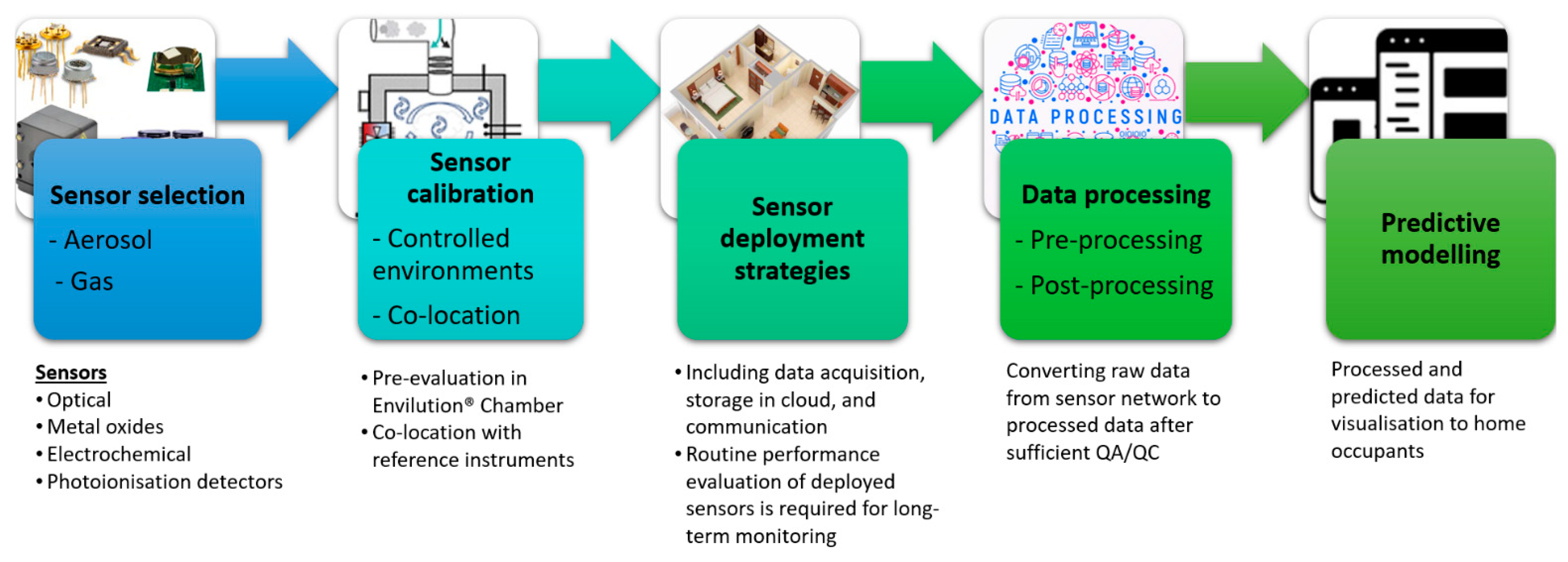
Table 1.
The unhealthy exposure thresholds defined for the common indoor and outdoor air pollutants [11,12,13].
| Pollutants | Indoor Air | Outdoor Air | References |
|---|---|---|---|
| Benzene (C6H6) [µg m−3] | Carcinogenic compounds, no safe level of exposure recommended risk of leukaemia estimated as 6 × 10⁻⁶ at 1 µg m−3, World Health Organisation (WHO). | 5 (annual) European Union (EU) 1.7 (annual) WHO | [13,14] |
| CO [mg m−3] | 100 (15 min–once per day) 35 (1 h–once per day) 10,000 (8 h) 7 (24 h) all from WHO. | 10 (max daily 8 h mean) EU 30 (1 h) WHO 10 (8 h) WHO | [13,14] |
| CO2 [ppm] | <1000 (hygienically harmless) 1000–2000 (elevated) >2000 (hygienically unacceptable) all from AIR. | 405 (by climate.gov, accessed on 21 March 2021) | [15] |
| HCHO [µg m−3] | 100 (30 min) WHO | N/A | [13] |
| Naphthalene [µg m−3] | 10 (annual) WHO | N/A | [13] |
| NO2 [µg m−3] | 200 (1 h) WHO 40 (annual) WHO | 200 (1 h) EU/WHO 40 (annual) EU/WHO | [13,14] |
| O3 [µg m−3] | N/A | 120 (max daily 8 h mean) EU 100 (8 h) WHO | [14,16] |
| PAH (benzo[a]pyrene) [µg m−3] | All indoor exposures relevant to health, lung cancer with risk of 8.7 × 10⁻⁸ at 1 µg m−3. | 1 (annual) EU 0.12 (annual) WHO | [13,14] |
| PM2.5 [µg m−3] | 10 (annual) WHO 25 (24 h) WHO | 10 (annual) WHO 25 (24 h) WHO 25 (annual) EU | [13,14,16] |
| PM10 [µg m−3] | 20 (annual) WHO 50 (24 h) WHO | 20 (annual) WHO 50 (24 h) WHO 40 (annual) EU 50 (24 h) EU | [13,14,16] |
| Tetrachloroethylene [µg m−3] | 250 (annual) | N/A | [13] |
| Trichloroethylene [µg m−3] | Carcinogenicity with risk of 4.3 × 10⁻⁷ at 1 µg m−3 | N/A | [13] |
| TVOCs a [mg m−3] | <0.3 (no hygienic objections) >0.3–1 (no relevant objections) >1–3 (some objections) >3–10 (major objections) >10–25 (not acceptable) | N/A | [17] |
Note: N/A refers to not available; AIR refers to German Committee on Indoor Guide Values, formerly known as “Ad-hoc AG”. a Total VOCs, defined by the International Organisation for Standardisation (ISO) 16000-6.
Table 2.
The current available air quality LCSs characteristics, advantages and disadvantages [39,40,42,43]. Examples of different deployed environmental and air pollution LCSs suggested for indoor environments are presented at the end of table.
| Sensor Technology | Known for | Summary of Pros and Cons |
|---|---|---|
| Electrochemical | NO2, SO2, O3, NO, CO, NH3 and VOCs 1 | √ Good sensitivity, from mg m−3 (potentiometric) to µg m−3 (amperometric). √ Fast response time (30–200 s). 2 √ Small in size (20 mm) and low power consumption (µW). √ Long-term stability with acceptable drift values (between 2% and 15% per year) reported for the commercial ECs. × Large in size, complicated, vulnerable to poisoning, and shorter life span (~1–3 years). × Highly sensitive to change in meteorology (temperature and RH variations) depending on electrolyte. 3 × Show cross-reactivity with similar molecule types. × More expensive than MOx gas sensors. |
| MOx | CO, CO2, H2, O3, NH3, NO, NO2, NOx, CH4, C3H8 and VOCs 4 | √ Good sensitivity, from mg m−3 to µg m−3 (ppb level) and relatively long lifetime (>5 years). √ Small in size (few millimetres) and long-lasting/light weight (few grams). √ Least power intensive (<1 W) – but higher than PIDs. × Results are affected by temperature and RH variations. × Long response time (>30 s; some cases 5–50 min), long stabilisation period before measurements (~24 h), and longer-term performance drift. × Poor recovery to achieve initial status under a change in experimental condition or exposure to a high concentration of target gases. × Output depends on the history of past inputs. × Instability over time. 5 |
| PID | VOCs 1 | √ Small in size with moderate price (approximately 400€ for a sensor to ~5000€ for a handheld device). √ Good sensitivity, down to mg m−3, some down to µg m−3. √ Limited temperature dependence and RH effects. √ Very fast (a few) response time. × Not selective: reacts to all VOCs that can be ionised by the UV lamp. Proper calibration and maintenance may be needed. × Significant signal drift. |
| Optical particle counter | PMs | √ Fast response time (in a second). √ Sensitivity in the range of 1 µg m−3. √ Able to identify the size of the particle in the size of PM10 and PM2.5. × Conversion from PM counts to PM mass with the theoretical model. × The measured signal depends on a variety of parameters such as particle shape, colour and density, RH, refractive index, etc. × Unable to detect ultrafine particles. 6 |
| Optical | CO and CO2 | √ Good sensitivity for CO2 (350–2000 ppm). √ Selectivity is good through characteristic CO2 IR spectra. √ Response time 20–120 s. √ Limited drift over time of the sensor calibration. × Need for correction for the effects of temperature, RH and pressure. |
| 1 Photoionisation detectors (PIDs) demonstrate a better sensitivity than electrochemical cells for volatile organic compounds (VOCs) (range from 100 ppb and 20 ppm). 2 Depend on the air temperature [40]. 3 The interference caused by temperature influence can be compensated. 4 MOx should not be used to measure low concentrations of VOCs in the presence of high concentrations of NO, NO2 or CO. MOx sensors are suitable when sensing VOCs, which are not detected by PIDs (e.g., many chlorofluorocarbons (CFCs)) [40]. 5 An empirical relation for drift or stability corrections have been suggested [40,44]. 6 No LCS is available that could detect ultrafine particles (<100 nm in diameter), because the optical systems are unable to detect <300 nm particles [42]. Note 1: Near real-time monitoring in indoor environments is required to capture the immediate incidents and to adopt precautionary and corrective measures, but not all the sensors discussed above are fast/immediate responsive enough to concentration changes. Currently, a reasonable average time among the deployed sensors is 30-s and/or 1-min averaging timestamp as per published studies in the literature. Besides, a balance should be maintained between sampling frequency and power source. Note 2: There are LCSs for other pollutants, such as Radon, NO, H2S, and SO2 which are not listed in here. Note 3: Here are some sensors that have been used in IAQ studies:
| ||
Table 3.
Specification of sensor-based product specifications (both single- and multiple-purpose units) reported by manufacturers available in the market that could be used for IAQ and/or personal indoor exposure monitoring systems. The authors highly suggest the buyers to check the up-to-date specifications of the sensors prior to selection and do not endorse any brand or a product.
| Single-Purpose Units Designed for IAQ | |||
| Sensor name | Pollutant | Technology | Specific Practical Features |
| Aeroqual S500 (OZU) | Can be used with a wide range of gas sensor heads (e.g., CO, CO2, O3, VOCs, PM2.5 and PM10). | A sensitive MOx that relies on the conductance of heated tungstic oxide (WO3). | Battery: Yes (12Vdc 2700 mA.h) Sampling mechanism: Air pump Sampling interval: N/S Environmental operating conditions –5 to 45 °C; up to 95% of RH Internal data storage/wireless communication: Yes/Yes Calibration: Zero and span calibration |
| AirAssure by TSI | Real-time measurements of PM2.5 mass concentrations. | Enable a light-scattering photometer that detects and measures PM2.5 between 5 and 300 µg m−3. | Power supply: Yes (24 V, 5 W max) Sampling mechanism: Air pump Sampling interval: N/S Environmental operating conditions: 10 to 30 °C; <65% Internal data storage/wireless communication: No/Yes Calibration: Pre-calibrated sensor with the National Institute of Standards and Technology (NIST) Statement of Conformance |
| AirBeam2 by HabitatMap | Measures PM1, PM2.5 and PM10, temp. and RH. | Use a light-scattering method to measure PMs. Particle sensor (Plantower PMS7003); RH sensor (Honeywell HIH-5030-001); Temp. sensor (Microchip MCP9700T-E/TT) | Battery: Yes (up to 10 h battery life) Power supply: Yes - micro universal serial bus (USB) port Sampling mechanism: Air pump Sampling interval: N/S Environmental operating conditions: N/S Internal data storage/wireless communication: No/Yes Calibration: Pre-calibrated by the manufacturer |
| Alphasense OPC- Particulate Monitor | Measures PM1, PM2.5 and PM10. Certified with ISO 9001:2015. | Use laser beams to detect particles from 0.38 micron to 17 micron in diameter. | Power supply: No battery, 175 mA Sampling mechanism: Air pump Sampling interval: Histogram period (1–30 s) Environmental operating conditions: up to 50 °C; up to 95% Internal data storage/wireless communication: Yes/No Calibration: Pre-calibrated by the manufacturer |
| AS-LUNG portable | Real-time measurements of PM1, PM2.5 and PM10 in µg m−3 as well as CO2 concentrations. | Use Plantower PMS3003 laser particle counter sensors, which come factory calibrated. | Battery: No (Yes for the station) Power supply: Yes, DC-5V Sampling mechanism: Air pump Sampling interval: N/S Environmental operating conditions: N/S Internal data storage/wireless communication: Yes/Yes Calibration: Pre-calibrated by the manufacturer |
| Cair | Detect dust particle concentration of a given size range in pcs ft−3. It measures VOC in ppm level, air temp. and RH. | Count particle via laser beams | Power supply: No battery, yes (USB 5 V) Sampling mechanism: Air pump Sampling interval: 1 min Environmental operating conditions: N/S Internal data storage/wireless communication: No/Yes Calibration: Pre-calibrated by the manufacturer |
| Cairsense micro-sensors | Offers a separate range of air quality gas sensors, including T, RH, NO2, NH3, CO, O3+NO2, NH3, H2S+CH4S, HCHO, SO2, PMs, and non-methane VOCs. | See Technical Data of each sensor kit for detailed specifications. | Battery: Yes Power supply: 5 VDC/500 mA Sampling mechanism: Air pump Sampling interval: 1, 15, and 60 min Environmental operating conditions: up to 40 °C; up to 100% Internal data storage/wireless communication: Yes/Yes Calibration: Pre-calibrated by the manufacturer |
| Dylos - DC1700-PM | Measures both PM2.5 and PM10 number (>0.5 µm and >2.5 µm) and mass concentrations interchangeably. | Use a true laser particle counter, where laser beams detect particles going past by their reflectivity. | Battery: Yes (up to 6 h of continuous use) Power supply: Yes Sampling mechanism: Air pump Sampling interval: Minimum for 1 min Environmental operating conditions: N/S Calibration: Pre-calibrated by the manufacturer |
| Eco Witt WH43 | Designed to provide real-time measurements of PM2.5 mass concentrations. | Use Honeywell HPM Series Particulate Sensor to detect/count particles using light-scattering between 0–999 µg m−3. | Battery: Yes Power supply: Yes (USB power cable) Sensor lifetime: 10 years for the Honeywell HPM Series PM2.5 sensor Sampling mechanism: Air pump Sampling interval: N/S Environmental operating conditions: N/S Internal data storage/wireless communication: No/Yes Calibration: Pre-calibrated by the manufacturer |
| Laser Egg | A handheld device that provides real-time measurements of PM2.5 and PM10. | Use light-scattering to measure particles between 0.3 and 10 micron within 10–100 ms in aerodynamic diameter. | Battery: Yes Battery Life: 8 h Power supply: DC 5 V (USB charging cable) Sampling mechanism: Air pump Sampling interval: N/S Environmental operating conditions: N/S Internal data storage/wireless communication: No/Yes Calibration: Pre-calibrated by the manufacturer |
| Micro Aeth | Model AE51 aethalometer, BC aerosol monitor that measures 0–1 mg BC m−3 | Measures the rate of change in absorption of transmitted light due to a continuous collection of aerosol deposit on T60 (Teflon coated glass filter). | Battery: Yes Power supply: Yes (5 V DC/0.5 A) Sampling mechanism: Internal pump up to 200 mL min−1 Sampling interval: 1, 10, 30, 60, or 300 s Environmental operating conditions: 0 to 40 °C Internal data storage/wireless communication: Yes/Yes Calibration: Pre-calibrated by the manufacturer |
| MicroPEM by RTI | A portable sensing device that measures PM2.5 and PM10. | It combines real-time nephelometry and integrated referee filter PM measurements. The device carries an impactor and a light-scattering particle detector. | Battery: Yes (up to 40 h of continuous operation) Power supply: Yes (120 V AC/60 Hz AC adapter to USB) Sampling mechanism: Pump (500 mL min−1) Sampling interval: 10 s Environmental operating conditions: N/S Internal data storage/wireless communication: Yes/Yes Calibration: Pre-calibrated by the manufacturer |
| Naneos - Partector | A portable, battery-powered instrument that measures the lung deposited surface area (LDSA) of nanoparticles. | Measures nanoparticle surface area based on a non-contact electrical detection principle. | Battery: Internal rechargeable Li:Ion battery (15 h) Power supply: USB charger (to either charge or run indefinitely) Sampling mechanism: Air pump (0.5 L min−1) Sampling interval: N/S Environmental operating conditions: N/S Internal data storage/wireless communication: Yes/No Calibration: Pre-calibrated by the manufacturer |
| POM * by 2B Technologies | Personal Ozone Monitor (POM) 4 ppb–10 ppm, Resolution 0.1 ppb | Absorption of ultraviolet light at 254 nm Baseline drift <2 ppb per day, <5 ppb per year Sensitivity drift <1% per day, <3% per year | Battery lifetime: 5–8 h Power supply: Yes Sampling mechanism: Air pump (0.75 L min−1) Sampling interval: 10 s, 0.1 Hz (Fast mode: 2 s, 0.5 Hz) Environmental operating conditions: up to 50 °C Internal data storage/wireless communication: Yes/Yes Calibration: Pre-calibrated by the manufacturer |
| PurpleAir PA-II (IAQ and OAQ) | An OPC, which measures PM1, PM2.5 and PM10 mass concentrations from the counts. | Use Plantower PMS5003 laser particle counter (maximum range ≥1000 μg m−3), where laser beams detect particles going past by their reflectivity. | Power supply: 5 V DC, 3 A Sampling mechanism: Air pump Sampling interval: N/S Environmental operating conditions: N/S Internal data storage/wireless communication: No/Yes Calibration: Pre-calibrated by the manufacturer |
| PurpleAir PA-I-Indoor | Use PMS1003 laser particle counters (maximum range ≥1000 μg m−3) where laser beams detect particles going past by their reflectivity. | Power supply: 5 V DC, 3 A Sampling mechanism: Air pump Sampling interval: N/S Environmental operating conditions: up to 60 °C; up to 99% Internal data storage/wireless communication: No/Yes Calibration: Pre-calibrated by the manufacturer | |
| Samyoung S&C SY-DS-DK3 | Designed to provide real-time measurements of PM2.5 mass concentrations. | The PM2.5 sensor provides mass concentration over 0.3 µm sized particles through Samyoung S&C’s proprietary optical structure with Infrared emitting diode. | Power supply: Yes Sensor lifetime: min. 5 years Sampling mechanism: Air pump Sampling interval: 2 s Environmental operating conditions: up to 65 °C; up to 95% Internal data storage/wireless communication: N/S Calibration: Pre-calibrated by the manufacturer |
| Sensirion - SPS30 Eval Kit | Real-time PMs mass/number concentrations. Mass concentration: PM1.0, PM2.5, PM4 and PM10 Number concentration: PM0.5, PM1.0, PM2.5, PM4 and PM10 | Based on laser scattering (1 to 1000 μg m−3) by using advanced particle size binning | Power supply: Yes Sensor lifetime: >8 years, operating continuously for 24 h/day Sampling mechanism: Air pump Sampling interval: 1 s Environmental operating conditions: 10 to 40 °C; 20% to 80% Internal data storage/wireless communication: N/S Calibration: Pre-calibrated by the manufacturer |
| Speck by Airviz | Detects fine PM (between 0.5 and 3.0 micron) in indoor environments. | Equipped with an optical sensor (DSM501A) that counts the number of particles per litre of air (ppl). It can estimate the particle mass per cubic meter of air (µg m−3). | Power supply: Micro USB, 5 V 500 mA Sampling interval: 5 s to 4 min (default 1 min) Environmental operating range: −10 ~ +65 °C; <95% Internal data storage/wireless communication: Yes/Yes Calibration: Pre-calibrated by the manufacturer by exposing to two controlled particle concentrations |
| Multipurpose units designed for IAQ | |||
| Sensor name | Pollutants | Technology | Specific Practical Features |
| +IQAir - AirVisual Pro | A handheld device that provides real-time measurements of PM (0.3–2.5 μm) and CO2 (400–10,000 ppm). | Use a light-scattering method to measure PMs. | Battery: Rechargeable Li:Ion (up to 4 h on a single charge) Screen Size: 5″ light-emitting diode (LED) Sampling mechanism: Air pump Sampling interval: N/S Operating temp.: 0 to 40 °C; 0 to 95% Internal data storage/wireless communication: No/Yes Calibration: Pre-calibrated by the manufacturer |
| Air Fruit | A handheld device that provides real-time measurements of PM2.5, CO2, temp. and RH. | Use light-scattering to measure PM2.5. PM2.5: 0~500 μg m−3 CO2: 0~10,000 ppm | Power supply: 5 V USB cable Sampling mechanism: Air pump Detection time interval: daytime 15 min / night 1 h Sampling interval: N/S Environmental operating conditions: up to 70 °C; <100% Internal data storage/wireless communication: No/Yes Calibration: Pre-calibrated by the manufacturer |
| Air Quality Egg V2 2020 | Used for measurements of CO2, SO2, CO, O3, PM (PM1, PM2.5 and PM10) and NO2 (not all together). Each set of sensors also monitors temp., pressure and RH. | Dual Plantower PMS5003 sensor ranges between 0.3 and 10 μm. | Power supply: No battery, 5 V USB or Micro-USB Sampling mechanism: Air pump Sampling interval: N/S Environmental operating conditions: up to 40 °C; up to 95% Sensor response time: Maximum of 30 s Sensor lifetime: 3 years Internal data storage/wireless communication: Yes/Yes Calibration: For gases, using previously calibrated electrochemical gaseous sensors |
| Airthings Wave Plus | A smart air quality monitor capable of measuring temp., RH, TVOCs, air pressure, radon and CO2. | Sensor specifications (except for CO2 which is NDIR) are not included in the product sheet. Settling time: TVOC ~7 days CO2 ~7 days | Battery: Yes, 2 AA 1.5 V Power supply: No Sampling mechanism: N/S (diffusion for radon) Sampling interval: 5 min Environmental operating conditions: 4 to 40 °C; <85% Internal data storage/wireless communication: No/Yes (Bluetooth or AirthingsSmartLink) Calibration: Pre-calibrated by the manufacturer |
| AirThinx IAQ | Real-time measurements of PM1, PM2.5 and PM10 in µg m−3. It also provides temp., RH, pressure, CO, CH2O and TVOC measurements. Holds Conformitè Europëenne (CE), Federal Communications Commission (FCC), PCS Type Certification Review Board (PTCRB) certificates. | Equipped with a factory calibrated Plantower PMS5003 laser particle counter. CO2: 0~3000 ppm PMs: 0~500 μg m−3 CH2O: 0~1 mg m−3 TVOC: 1~30 ppm of EtOH | Power supply: Yes (5 V DC) Sampling mechanism: Air pump Sampling interval: 1, 5, 10, 15, and 30 min Environmental operating conditions: up to 75 °C Internal data storage/wireless communication: No/Yes (incl. cellular) Calibration: Pre-calibrated by the manufacturer |
| Awair | Real-time measurements of temp., RH, CO2, PM2.5 and chemicals (VOC). It needs Wi-Fi for setup. | Senso specs: Temp. −40 to 125 °C RH 0 to 100% CO2 400–5000 ppm PM2.5: 0–1000 µg m−3 VOCs: 0–60,000 ppb | Battery: No Power supply: 5 V/2.0 A external power adapter Sampling mechanism: N/S Sampling interval: 5 min Environmental operating conditions: N/S Internal data storage/wireless communication: No/Yes Calibration: Pre-calibrated by the manufacturer |
| Blueair Aware | The Blueair Aware is a standalone air quality monitor to measure T (0 to 50 °C), RH (25% to 75%), CO2 (450 to 5000 ppb), PM2.5 (1 to 500 μg m−3), and TVOC (125 to 1000 ppb). | N/R | Power supply: Yes (Non-detachable USB cable) Sampling mechanism: Air pump Sampling interval: 5 min Environmental operating conditions: 0 to 50 °C; 5 to 95% Internal data storage/wireless communication: No/Yes Calibration: Pre-calibrated by the manufacturer |
| Edimax | The Edimax Edigreen Home sensor measures PM2.5 and PM10 in µg m−3, CO2, HCHO, TVOC, temp. and RH. | Use a Plantower PMS5003 laser particle counter, which comes factory calibrated. PM2.5/10: 0–500 μg m−3 PM10: 0–500 μg m−3 CO2: 400–2000 ppm TVOC: 0–1000 ppb HCHO: 0–1 mg m−3 | Power supply: Yes (USB power adapter) Sampling mechanism: Air pump Sampling interval: N/S Environmental operating conditions: 0 to 50 °C; 0 to 100% Internal data storage/wireless communication: No/Yes Calibration: Pre-calibrated by the manufacturer (CO2 and TVOC sensors require up to 72 h to self-calibrate after the installation). |
| Huma-i (HI-300A) | Advanced Portable Air Quality Monitor Indoor and Outdoor Measures temp., RH, CO2, VOC, PM1, PM2.5, and PM10. | CO2 (400~5000 ppm) VOC (0.000~10 ppm) PM1, PM2.5 and PM10 (0~1000 µg m−3) CE and FCC certification | Battery: Yes, built-in Li-polymer @ 650 mAh/3.7 V Power supply: AC 100/240 V, 50/60 HZ, USB-C Sampling mechanism: Air pump Sampling interval: N/S Environmental operating conditions: –10~60 ℃; 0~99% Internal data storage/wireless communication: Yes (90 days)/Yes Calibration: Pre-calibrated by the manufacturer |
| IDEAL AS10 | The IDEAL AS10 indoor air sensor measures the air composition, indoor climate and possible environmental impacts, all in real time. | It measures PM2.5 and PM10 (0–1000 μg m−3), VOCs (0–32,768 ppb), temp (–10 to +50 °C), RH (20–90%) and air pressure (20–110 hPa). | Battery: No Power supply: 5 V micro USB cable Sampling mechanism: N/S Sampling interval: 1 s Transmission interval: 60 s Environmental operating conditions: Up to 50 ℃; 20~90% Internal data storage/wireless communication: No/Yes Calibration: Pre-calibrated by the manufacturer valid for 24 months |
| Laser Egg +chemical or +CO2 | A handheld device that provides real-time measurements of temp., RH, PM2.5 and VOCs or CO2. | Use light-scattering to measure particles between 0.3 and 2.5 micron. | Battery: Yes Battery Life: 8 h Power supply: DC 5 V (USB charging cable) Sampling mechanism: Air pump Sampling interval: N/S Environmental operating conditions: N/S Internal data storage/wireless communication: No/Yes Calibration: Pre-calibrated by the manufacturer |
| Magnasci SRL - uRADMonitor A3 (HW105) | Measures 8 air quality parameters including PM2.5, CO2, VOC, HCHO, temp., RH, barometric pressure and Gamma/X-ray radiation. | Use laser scattering sensor to detect PMs; a NDIR sensor to measure CO2; an EC for HCHO, a Bosch BME 680 sensor for temp., RH, barometric pressure and VOC; and an S129BG Geiger Tube to detect gamma and X-ray radiation. | Battery: No Power supply: 6–28 V Sampling mechanism: Air pump for active flow Sampling interval: N/S Environmental operating conditions: up to 85 °C, up to 100% Internal data storage/wireless communication: No/Yes Calibration: Pre-calibrated by the manufacturer |
| SainSmart - Pure Morning P3 | Measures PM2.5, HCHO, CO2, air temp. (in °C) and RH (%). | Equipped with a Plantower PMS5003 laser particle counter. | Battery: No Power supply: Yes (5 V) Sampling mechanism: Air pump Sampling interval: N/S Environmental operating conditions: N/S Internal data storage/wireless communication: No/Yes Calibration: Pre-calibrated by the manufacturer |
| Temtop M2000 | Measures real-time reading of HCHO, PM2.5, PM10, CO2, temp. and RH. | PM2.5 range: 0~999 μg m−3 PM10 range: 0~999 μg m−3 CO2 range: 0~5000 ppm HCHO range: 0~5 mg m−3 | Battery: Yes Power supply: 5 V DC Sampling mechanism: Air pump Sampling interval: N/S Environmental operating conditions: up to 50 °C; <90% Internal data storage/wireless communication: Yes/No Calibration: Pre-calibrated by the manufacturer |
| uHoo | Carries eight dedicated sensors for VOCs (10–10,000 ppb), PM2.5 (0–200 µg m−3), CO (0–1000 ppm), CO2 (400–10,000 ppm), O3 (10–10,000 ppb), temp. (–40 to 85 °C), RH (0 to 100%) and air pressure (300–1100 mbar). | Battery: No Power supply: Yes, 5 V DC Sampling mechanism: Air pump Sampling interval: N/S Internal data storage/wireless communication: No/Yes Calibration: Pre-calibrated by the manufacturer | |
* Designated by US EPA as a Federal Equivalent Method (FEM: EQOA-0815-227). Note 1: Sensors’ lifetime of the reviewed kits is not reported in the technical documents. Note 2: N/S and N/R stand for not specified and not reported, respectively.
Table 4.
Some recent LCS deployments indoors across the world.
| Pollutants/Range of Operation | Sensor Type | Room Size | Reference Instrument | Sensor Placement/ Country | Sampling Frequency | Correlation Factor R2/Agreement | Duration | References |
|---|---|---|---|---|---|---|---|---|
| PM1, PM2.5, PM10 | PM-Model-II particle counters (Plantower PMS3003) | 88 m2 | Particle monitor (Thermo Scientific Model FH 62 C14) | An apartment in Beijing | 1 min resolution | 79% of the spatiotemporal variation based on a regression model | 10 days | [81] |
| PM1, PM2.5, PM10 | Dylos DC1100 Pro and Plantower PMS sensor (AirU) | Two homes, 306.6 m2 and 140 m2 | GRIMM, DustTrak, and MiniVol | Two households in Salt Lake City, USA | 1 min | See various R2 in the manuscript | One-week calibration, several weeks for sampling | [82] |
| PM2.5 and PM10 from 21 common residential sources | Air Quality Egg 2018; IQAir AirVisual Pro (AVP); Awair 2nd Edition; Kaiterra Laser Egg; PurpleAir Indoor; and Ikair | N/R | Grimm Mini Wide-Range Aerosol Spectrometer Model 1371 | N/R | 5 min | R2 ≥ 0.83 | 48 h | [83] |
| CO (0-29), CO2 (0-3600), PM10/2.5 (0-1) and VOC (0-46) * | Aeroqual Series 500 with different sensor heads. gas-sensitive electrochemical (GSE), NDIR, laser particle counter, and PID types | Floor area of merely 9.3 m2 | Not applicable | Subdivided unit (SDU) in Hong Kong | 60, 120, 5, and 30 sec | No significant correlation between indoor and outdoor pollutants in case of CO (3.58%), PM10 (0.96%), and PM2.5 (7.11%). | 48 h in each SDU in the summer of 2018 | [84] |
| Noise (35–120 dB), T (0–50 °C), RH (0–100%), CO (0–1000 ppm), CO2 (0–5000 ppm), NO (0–20 ppm), NO2 (0–20 ppm) and PM2.5 (0.38–17 μm) | Netatmo Weather Station, Onset Temperature, Alphasense (COB4, NOB4, NO2B43F, and OPC-N2), and Harvard miniPEM | In a residential building | RTI MicroPEM for PM only (5 min avg.) | Boston, MA, USA | 1 min | Carried out only for PM2.5 (Lab (TSI SidePak™ AM510): R2 = 0.47; field (RTI MicroPEM): R2 = 0.83) | Multiple 1-week sessions | [71] |
| CO, NO2, NO, O3, PM2.5 (PAM, Model AS520) | 4-electrode ECs (Great Notley, UK): CO-A4 (for CO), NO2-A43F (for NO2), NO-A4 (for NO), and Ox-A431 (for O3). For PM: a miniaturised OPC (OPC-N2, Alphasense) | A living room | BLUME instrumentation uses chemiluminescence to measure NO2 and NO, UV absorption for O3, non-dispersive infrared absorption for CO, and particle light-scattering for PM2.5 (model EDM180, Grimm Aerosol Technik, Ainring, Germany). | The indoor instrument was placed into the home’s living room, which was either adjacent to the back garden or separated from it by a room in between. | Maximum: 1 Hz. Minimum: 20 sec (PM). | For the inorganic gases (0.92 < R2 < 0.96) for PM2.5 (R2 = 0.64) | Simultaneous indoor pollutant measurements in residential buildings in Berlin, Germany. Instruments measured one week per location. | [85] |
| Ammonia (1–500 ppm), CH4 (>1000 ppm), C3H8 (>1000 ppm), C4H10 (>1000 ppm), CO (1–1000 ppm), Ethanol (10–500 ppm), H2 (1–1000 ppm), NO2 (0.05–10 ppm) | MOx sensors (MICS series) | Real-time IAQ monitoring in a home using iAir | N/R | Guarda, Portugal | 30 sec | N/R | N/R | [86] |
| CO and PM2.5 | HAPEX and TZOA-R for PM2.5 EL-USB-C for CO | 1 m from an indoor fireplace and 0.6 m above the ground | DustTrak DRX (Model 8534) BGI/Mesa Labs pump (Model BGI4004) Q-Trak (Model 7575) | Non-smoking private single-family house/Spain | 5 min | R2 up to 85 | 5 days | [87] |
| CO and PM2.5 | HAPEX (PM2.5) and EL-USB-C (CO) | Main living area at least at 1 m above the ground | SKC pump (Model Universal PCXR8) | 4 households located in 4 villages/India March-April 2016 | 5 min | N/R | 1 week | [87] |
| PM2.5 (25 µg m−3), tVOC (300 ppb), CO2 (1300 ppm), T (40 °C), and RH (60%) | Foobot kit | An occupied bedroom (floor area 10.5 m2) of a modern flat | GrayWolf TG-502 TVOC, IQ-410, and PC-3016A | Glasgow, UK | 5 min | A significant agreement with the GrayWolf T (rs = 0.83–0.87) RH (rs = 0.94–0.95) tVOC (rs = 0.83–0.87) PM2.5 (rs = 0.79–0.87) | 81 h 25 min (from 28 August 23:50 LT to 1 September 2017 11:25 LT) | [88] |
| PM, CO, O3, NO2, noise, temp. and RH | A dust sensor (Sharp, Model DN7C3CA006, Osaka, Japan) A 4-electrode CO sensor (Alphasense, Model CO-B4 with sensor board 000-01SB-02, Essex, UK) A 4-electrode oxidizing gas sensor (Alphasense, model OX-B431 with sensor board 000-01SB-02, Essex, UK) A temp. and RH sensor (Adafruit, model AM2302, NY, USA) A custom-built noise level sensor | DataRAM 1500 Aerosol Monitor (Thermo Fisher Scientific., pDR, Shoreview, MN, USA) for PM Q-Trak Plus 8552 (TSI Inc., Shoreview, MN, USA) for CO, POM (2B Technologies Inc., PO3M, Boulder, CO, USA) for O3 A sound level meter (NTi Audio, SLM, Schaan, Liechtenstein) for noise, | Within the fabrication area of a manufacturing facility | 5 min | 0.98 to 0.99 for particle mass densities up to 300 µg m−3 0.99 for CO up to 15 ppm. 0.98 for the oxidizing gas sensor (NO2) over the sensitive range from 20 to 180 ppb. 1% between 65 and 95 dBA. | Three months | [89] | |
| PM | Wireless PM sensor, Sharp GP2Y1010AU0F | Approximately 29 m2 of floor area | TSI Sidepak AM 150 (TSI Inc., Minnesota, USA) | 2 kitchens in Raipur, India | Sidepak 1 Hz and sensors 0.25 Hz | 0.71 | Multiple days at the two households | [35] |
| Light (0.1 to 40,000 Lux), T (−55–80 °C), RH (0–100%), CO2 (0–10,000 ppm) | TAOS TSL2561, Onset HOBO (NTC thermistor, Sensirion SHT15), SenseAir K-30 | IAQ in an educational building | N/R | Two locations at Illinois Institute of Technology in Chicago, IL | 1 min | N/R | 1 week | [33] |
1 Automatically control building climate control systems (air purifiers, kitchen hoods, bathroom or whole house fans, operable windows, or dampers in the mechanical room), when measured pollutant levels are higher than acceptable levels. * Concentration values are in mg m−3. Note: N/R represents not reported.
Table 5.
A summary of recent IAQ modelling studies that use various machine learning techniques for the prediction of IAQ parameters. Studies carried out in offices, schools and commercial buildings are excluded as their layouts could be different from residential buildings.
Table 5.
A summary of recent IAQ modelling studies that use various machine learning techniques for the prediction of IAQ parameters. Studies carried out in offices, schools and commercial buildings are excluded as their layouts could be different from residential buildings.
| Input to the Model | Model Output | Environment, Location, Date, Time | Model | Correlation | Recommendations | Reference |
|---|---|---|---|---|---|---|
| Time, in/out temp. and RH | Temp. and RH | A test house (147.8 m2 × 3 m) in Finland | Artificial neural networks or ANN (non-linear autoRegressive with eXternal input (NNARX) model and genetic algorithm were employed to construct networks) | Correlation coefficients 0.998 and 0.997 for temp. and RH | Three-layer feed-forward ANN is capable of predicting any nonlinear relations even in a complex situation where (i) some impact factors are still unclear and (ii) some important information is unavailable. | [175] |
| Resident activities | CO2 | Two smart apartments and a smart workplace, Washington State University, Pullman, WA, USA | Naïve Bayes, ANN and Decision tree | N/S | The decision tree algorithm did perform best in many examined cases. | [176] |
| Indoor temp. and RH | CO2 | 8 apartments (4 bedrooms and 6 living rooms) located in Kuopio, Finland, from May to October 2011. Measurements were taken every 10 s. | ANN (based on multilayer perceptron network) | R2 ≤ 0.39 ± 0.02 | The prediction of CO2 is difficult, if it is based only on measurements of RH and temp. | [168] |
| Temp., internal PM2.5 sources, window opening | PM2.5 | Dwelling (single-storey flats in England during October to May) | ANN (feed-forward) | R2 between 0.84 to 0.90 | ANN is able to accurately predict IAQ from a reduced set of input variables. | [177] |
| Temp. and RH | CO2 | Two rooms named as R203 and R204 of Smart Home | Decision tree regression/random forest | Accuracy of 46.25 ppm | It is possible to use the Random Forest method with sufficient accuracy in CO2 estimation on the basis of the internal and external temp./RH, the time and date as the input parameters. | [178] |
| Particle deposition parameters | PM2.5 | N/R | ANN (multilayer Perceptron) | N/R | ANN gives an average relative error of <5% | [179] |
| PM2.5, PM10, CO2, temp., and RH | Indoor airborne culturable bacteria | Data were measured in various buildings in Baoding, a city that suffers from PM2.5 pollution in China. | General regression neural network (GRNN) | N/R | A machine learning-based method can estimate the concentration of indoor airborne culturable bacteria. A well-trained GRNN model can help to quickly acquire the estimated concentration. | [180] |
| Ambient PM2.5 with 10 and 80 min of lag time | PM2.5 | Indoor and ambient PM2.5 in 13 households in Beijing, China. | Exponential regression | R2~0.87 | The PM2.5 concentrations can be predicted based on ambient measurements. The overall exposure would be overestimated without taking indoor air concentrations into consideration. | [181] |
| Temp. and RH | CO2 | In a room for almost a week (starting from 11 February 2015, to 18 February 2015) in Mons, Belgium | ANN (multilayer Perceptron) | <17 ppm difference on average to actual CO2 value | Open-loop and five-steps-ahead prediction networks had better MSE performances, higher sensitivity and specificity values vs. open- and closed-loop models. The CO2 concentration data are always needed to obtain acceptable predictions. | [166] |
| One dependent variable and 87 potential predictor variables | PM2.5 | 7-day PM2.5 measurements inside the homes of pregnant women from January 2014 to December 2015 in Ulaanbaatar, Mongolia | Multiple linear regression and random forest regression | Multiple linear regression (R2 = 50.2%) and random forest regression (R2 = 48.9%) | The improved performance of blended multiple linear regression/random forest regression models in predicting indoor air pollution. | [164] |
| PM10, PM2.5, CO2, temp., and RH | PM1 | Real-time daily IAQ monitoring in 10 households during March 2014 to July 2014, India. | Multiple linear regression | R2 = 0.81–0.98 | Multiple linear regression models were found to perform satisfactorily as indicated by 0.92 < index of agreement < 0.99 and 0.81 < R2 < 0.98. | [182] |
| Ambient PM2.5 and questionnaire-elicited information | PM2.5 | Daily average of PM2.5 during 3 consecutive days in summer and winter for 116 households in Hong Kong | Linear mixed regression | R2 = 0.61 by cross-validation | The fitted linear mixed-effects model is moderately predictive for the observed indoor PM2.5. | [183] |
Publisher’s Note: MDPI stays neutral with regard to jurisdictional claims in published maps and institutional affiliations. |
© 2021 by the authors. Licensee MDPI, Basel, Switzerland. This article is an open access article distributed under the terms and conditions of the Creative Commons Attribution (CC BY) license (https://creativecommons.org/licenses/by/4.0/).
Share and Cite
MDPI and ACS Style
Omidvarborna, H.; Kumar, P.; Hayward, J.; Gupta, M.; Nascimento, E.G.S. Low-Cost Air Quality Sensing towards Smart Homes. Atmosphere 2021, 12, 453. https://0-doi-org.brum.beds.ac.uk/10.3390/atmos12040453
AMA Style
Omidvarborna H, Kumar P, Hayward J, Gupta M, Nascimento EGS. Low-Cost Air Quality Sensing towards Smart Homes. Atmosphere. 2021; 12(4):453. https://0-doi-org.brum.beds.ac.uk/10.3390/atmos12040453
Chicago/Turabian StyleOmidvarborna, Hamid, Prashant Kumar, Joe Hayward, Manik Gupta, and Erick Giovani Sperandio Nascimento. 2021. "Low-Cost Air Quality Sensing towards Smart Homes" Atmosphere 12, no. 4: 453. https://0-doi-org.brum.beds.ac.uk/10.3390/atmos12040453
Note that from the first issue of 2016, this journal uses article numbers instead of page numbers. See further details here.