
Lattice Boltzmann Method-Based Simulations of Pollutant Dispersion and Urban Physics


1
Aix Marseille Univ, CNRS, Centrale Marseille, M2P2 UMR 7340, 13451 Marseille, France
2
Univ Lyon, CNRS, INSA-Lyon, Université Claude Bernard Lyon 1, CETHIL UMR5008, F-69621 Villeurbanne, France
*
Author to whom correspondence should be addressed.
Atmosphere 2021, 12(7), 833; https://0-doi-org.brum.beds.ac.uk/10.3390/atmos12070833
Submission received: 30 May 2021
/
Revised: 18 June 2021
/
Accepted: 22 June 2021
/
Published: 28 June 2021
(This article belongs to the Special Issue High Performance Computing Serving Atmospheric Transport & Dispersion Modelling)
Abstract
:Mesocale atmospheric flows that develop in the boundary layer or microscale flows that develop in urban areas are challenging to predict, especially due to multiscale interactions, multiphysical couplings, land and urban surface thermal and geometrical properties and turbulence. However, these different flows can indirectly and directly affect the exposure of people to deteriorated air quality or thermal environment, as well as the structural and energy loads of buildings. Therefore, the ability to accurately predict the different interacting physical processes determining these flows is of primary importance. To this end, alternative approaches based on the lattice Boltzmann method (LBM) wall model large eddy simulations (WMLESs) appear particularly interesting as they provide a suitable framework to develop efficient numerical methods for the prediction of complex large or smaller scale atmospheric flows. In particular, this article summarizes recent developments and studies performed using the hybrid recursive regularized collision model for the simulation of complex or/and coupled turbulent flows. Different applications to the prediction of meteorological humid flows, urban pollutant dispersion, pedestrian wind comfort and pressure distribution on urban buildings including uncertainty quantification are especially reviewed. For these different applications, the accuracy of the developed approach was assessed by comparison with experimental and/or numerical reference data, showing a state of the art performance. Ongoing developments focus now on the validation and prediction of indoor environmental conditions including thermal mixing and pollutant dispersion in different types of rooms equipped with heat, ventilation and air conditioning systems.
1. Introduction
The capability to accurately predict urban physics and environmental quality for citizens via numerical simulation is nowadays a critical challenge, since it is a key tool for designing future optimized and sustainable urban areas. Such predictive models should account for a very broad range of physical mechanisms, ranging from large-scale meteorological effects to very small scale unsteady fluctuations of physical quantities such as temperature, air velocity, pressure, humidity, etc.
Among the different interacting physical phenomena occurring in the atmosphere at the meso- and microscales are orographic effects, land sea breeze, urban heat islands, deep convection, thunderstorms, convection, thermals, building wakes and turbulence (see Figure 1 in Schlünzen et al. [1]). Mesoscale atmospheric flows that develop in the boundary layer or microscale flows that develop in urban areas are thus very complex, especially due to multiscale interactions, multiphysical couplings, land and urban surface thermal and geometrical properties and turbulence.
Accurately predicting these different atmospheric phenomena and their underlying physical mechanisms is challenging. It is even more the case in the urban roughness sublayer due to the intricate patterns of cities, generally composed of heterogeneous and dense layouts of numerous buildings and trees, as well as various types of surfaces, heat and moisture sources. However, accurately predicting these flows in cities is of the utmost importance, especially as urban air flows are determining pollutant dispersion, pedestrian wind comfort, and structural and thermal loads on buildings.
Therefore, a key feature of predictive numerical models is the capability to handle realistic full scale configurations (including geometrical details and physical mechanisms at play) via high-fidelity unsteady simulation techniques well suited for turbulent flows. Large eddy simulations (LESs [2]) have appeared as a promising numerical approach for that purpose, whose main limitation is related to the simulation complexity and numerical cost [3,4]. To alleviate this problem, Lattice Boltzmann Methods (LBMs [5,6]) have recently been identified as one of the most efficient approaches for “revolutionnary computational fluid dynamics (CFD)” [7] since they allow for a drastic reduction in (i) the computational time compared to classical CFD approaches based on the Navier–Stokes equations and (ii) the preprocessing step including the volumic mesh generation thanks to the coupled use of embedded Cartesian grids and immersed boundary conditions techniques.
The efficiency of LBM-based solvers to handle full scale urban flow simulations has been demonstrated by several authors. As an example, they have been used recently to simulate the flow in a km area of Tokyo to evaluate the gust index at pedestrian level [8] and the turbulence statistics [9]. These simulations were carried out in a complex geometry thanks to the use of Cartesian grids and the immersed boundary conditions strategy that permit drastically reducing the preprocessing cost. Thanks to its high efficiency in terms of parallel computing, the LBM is an attractive method for implementation on Graphic Processing Units (GPUs), which reduce the computational cost. The use of the LBM for implementing GPUs allows real time simulations of the flow over a build area [10] and the dispersion of a pollutant inside Oklahoma City [11] to be achieved with quite good accuracy. The efficiency of the LBM compared to a Navier–Stokes (NS) approach has been analysed in the case of the cross flow through an open window in an isolated cubical building. The comparison of the velocity field inside the building shows a good accuracy of both NS-LES and LBM-LES simulations compared to experimental data and the LBM simulation on GPU was up to 700 times faster than the NS simulations [12,13].
The goal of the present paper is to illustrate and summarize an innovative CFD LES approach for the simulation of atmospheric and urban flows, developed in the framework of the ProLB software [14,15] and based on the LBM. Already used to study the aerodynamics of vehicles and airfoils [16,17,18], the approach was adapted to deal with atmospheric and urban physics problems. Thanks to its formulation and the treatment of boundary conditions, the approach is computationally effective. It is thus possible to perform efficient but detailed and high-fidelity simulations of complex built environments with multiscale interactions and multiphysical couplings, in order to study a large scope of atmospheric and urban physics problems.
To illustrate the ability of the developed LBM-LES approach to study mesoscale and urban microscale atmospheric flows, including transport and dispersion processes, the paper is organized as follows. First, Section 2 synthesizes the main numerical aspects of the developed method. Then, Section 3, Section 4 and Section 5 summarize recent developments and validated studies performed using the hybrid recursive regularized (HRR) collision model for the simulation of complex or/and coupled turbulent atmospheric flows, including a micrometeorological model, with different applications. In particular:
- Section 3 reviews four applications of the developed method to the prediction of convective humid air flows with condensation with increasing meteorological likeness: a double diffusive Rayleigh Bénard convection (Section 3.1), rising two- and three-dimensional moist thermal bubbles (Section 3.2) and a shallow cumulus convection (Section 3.3).
- Section 4 reviews three use cases focusing on pollutant dispersion, considering different geometrical or physical complexity levels: neutral gas dispersion in a street canyon without or with tree planting effects (Section 4.1), neutral gas dispersion behind an isolated building without or with unstable thermal stratification (Section 4.2) and neutral or dense gas dispersion in a complex realistic urban environment (Section 4.3).
- Lastly, Section 5 reviews the validation and study of velocities (Section 5.1 and Section 5.3) and pressure distribution on building facades (Section 5.2 and Section 5.4) in a complex urban environment including high-rise buildings, with uncertainty quantification towards a more relevant assessment of pedestrian wind comfort and wind loads on urban buildings.
To conclude, Section 6 discusses the ongoing developments, especially regarding indoor dispersion problems with thermal and moving people effects, and Section 7 closes the present paper by summarizing the main findings of the different studies performed, highlighting the benefit of the current approach to support the development of fast response models and decision making.
2. The HRR-LBM-WMLES Numerical Model for Atmospheric Flows
This section summarizes the main elements of the developed LB-based numerical model. More details about the general LBM can be found in Krüger et al.’s work [5].
2.1. Generalities about LBM
The LBM mainly aims at simulating the macroscopic behaviour of fluids. However, as compared to the macroscopic description of the flow underlying common Navier–Stokes-based approaches, the LBM is based on a mesoscopic description of the flow. The fluid dynamics is simulated through streaming and collision steps based on the lattice Boltzmann equation:
where is a set of discrete velocities, usually a D3Q19 for three-dimensional problems (3 dimensions, 19 discrete velocities), is the discrete distribution function, and is the collision operator, i.e., the source term representing the redistribution of induced by collision. From this lattice Boltzmann equation, we can see that in practice only the first order neighbours are used in the algorithm, which permits increasing the parallel computation efficiency and allows the LBM to be faster than classical Navier–Stokes approaches.
Multiscale expansions show that the three-dimensional weakly compressible Navier–Stokes equations can be recovered to the second order by the LBM.
2.2. Key Features of the Present Lattice Boltzmann Method
Based on the general LBM framework, different developments were made in the ProLB solver to deal more efficiently with atmospheric and urban problems. In particular, the collision term was estimated using a regularized BGK model with a hybrid recursive procedure [19] as follows:
where , is the nonequilibrium part of the distribution function computed from the projection of distribution function on Hermite polynomials and is the nonequilibrium part of distribution functions approximated by finite differences. This procedure allows for both improved robustness as compared to usual BGK or MRT collision models and accuracy for large scale simulations, including urban and atmospheric flows.
Different forcing mechanisms (e.g., buoyancy, Earth rotation, etc.) can also be taken into account in the model following Guo et al. [20]. In particular, buoyancy forces (), due to differences in gas composition or temperature, can be modeled using a usual Boussinesq approach, as follows:
with:
where C is the concentration, is the reference concentration that is equal to 0, is the expansion coefficient of concentration, T is the temperature, is the reference temperature and is the expansion coefficient of temperature. Note that thermal buoyant flows can also be modeled thanks to the perfect gas law. Several other external forcings such as mesoscale or Coriolis effects can also be taken into account.
The domain boundaries are integrated using the cut cell method, which enables complex geometries to be modeled while substantially reducing the preprocessing costs (see Feng et al.’s work [21] for details), and a synthetic eddy method (SEM, [22]) was developed to generate inlet turbulence [23].
Since the LBM exhibits the same turbulent closure problems as the Navier–Stokes-based methods, classical subgrid models and wall models (WMs) for atmospheric flow simulations (including neutral, convective and stable cases) are used in the present solver, leading to the definition of the present HRR-LBM-WMLES tool for atmospheric flow simulation. Details are omitted here for the sake of brevity and can be found in Feng et al.’s work [24].
The developed approach also relies on a hybrid strategy to address more complex problems than purely aerodynamic problems, such as dispersion or thermal problems. This approach does not consider multidistributions, but the mass and momentum conservation equations are solved using the LBM, while the scalar transport equations are solved using a usual finite volume/finite difference method for the sake of efficiency. The corresponding temporal and spatial discrete coordinates are the same as the ones used for the LBM. Thus, it is possible to consider only one additional unknown per additional equation and optimize the numerical efficiency of the model.
3. Application of the Present HRR-LBM-WMLES to Convective Humid Boundary Layers with Cloud Formation
This section reviews different use cases studied to finally address large scale buoyant meteorological flows accounting for cloud dynamics thanks to a condensation scheme. More details can be found in Feng et al.’s work [25,26].
For these applications, the potential temperature () is defined as:
where is the air gas constant per mass unit, is the averaged mass heat capacity, is the reference pressure at ground and is the height-dependent reference state pressure.
The air was assumed as a mixture of liquid water (mass fraction ), water vapour (mass fraction ) and dry air (mass fraction ), the rate of phase change was assumed to be infinitely fast, and the two phases were assumed to be in thermo-chemical equilibrium. The vapour and liquid water were modeled following Equations (8) and (9).
where is a source term (typically the condensation) and is the water fraction diffusivity coefficient.
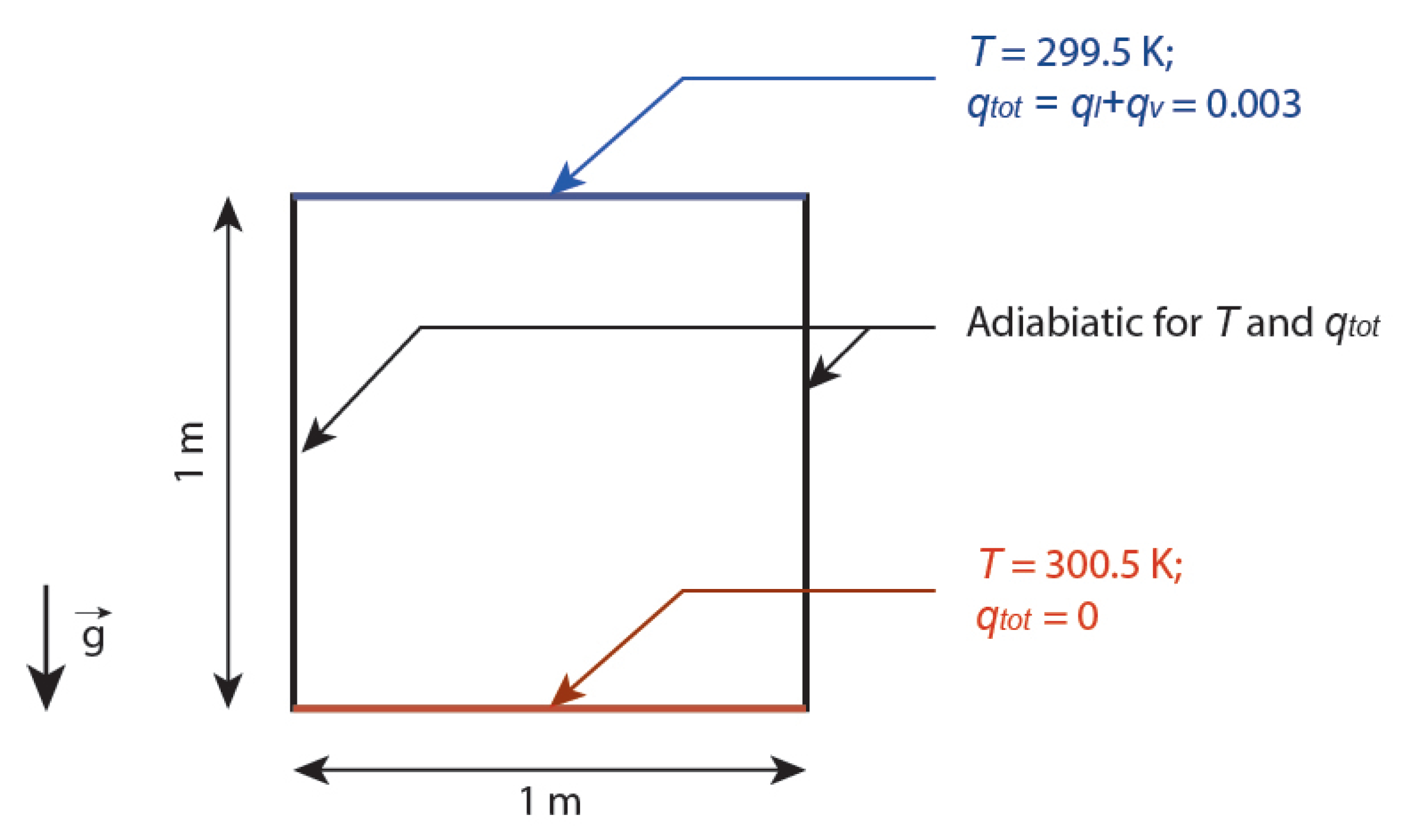
3.1. Double Convective Rayleigh-Bénard with Humid Air
The first validation case aims at validating the capability of the method to capture buoyancy effects, including both temperature and humidity gradients. It addresses the flow in a 2D square domain with temperature and humidity differences between its bottom and top boundaries as shown in Figure 1. Two Rayleigh numbers of and as well as two grids with or half and or half were considered. Condensation was neglected and details of the model settings can be found in Feng et al.’s work [25].
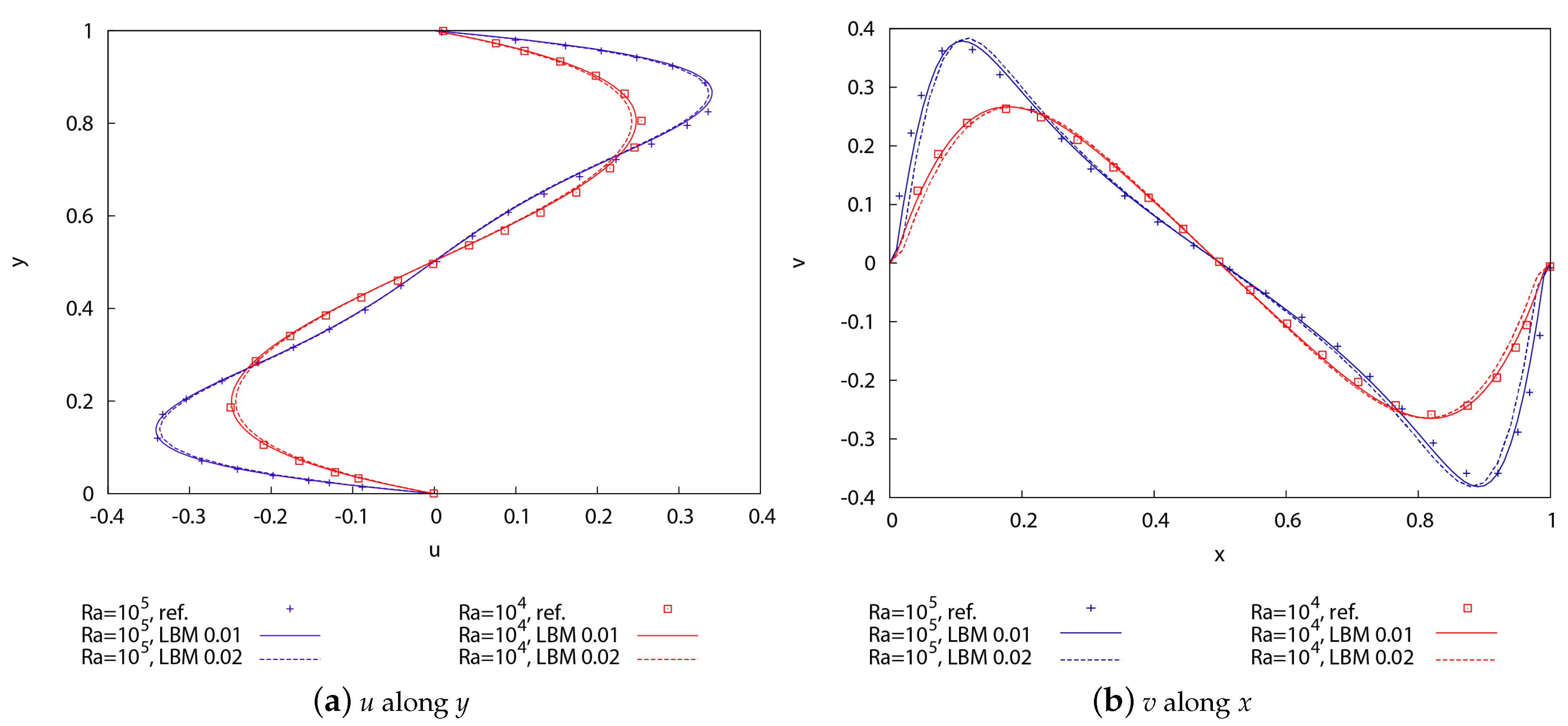
HRR-LBM simulation results were compared to the reference solution of Ouertatani et al. [27], which used a finite volume method discretized using the QUICK scheme in the momentum equation, and a second order central difference scheme in the energy equation, with a nonuniform grid of points.
The comparison between the simulated and reference velocity profiles along the domain midlines (Figure 2), as well as local Nusselt number through the hot wall, potential temperature and total water humidity contours when the steady state had been achieved (not shown here), highlights a good performance of the developed HRR-LBM.
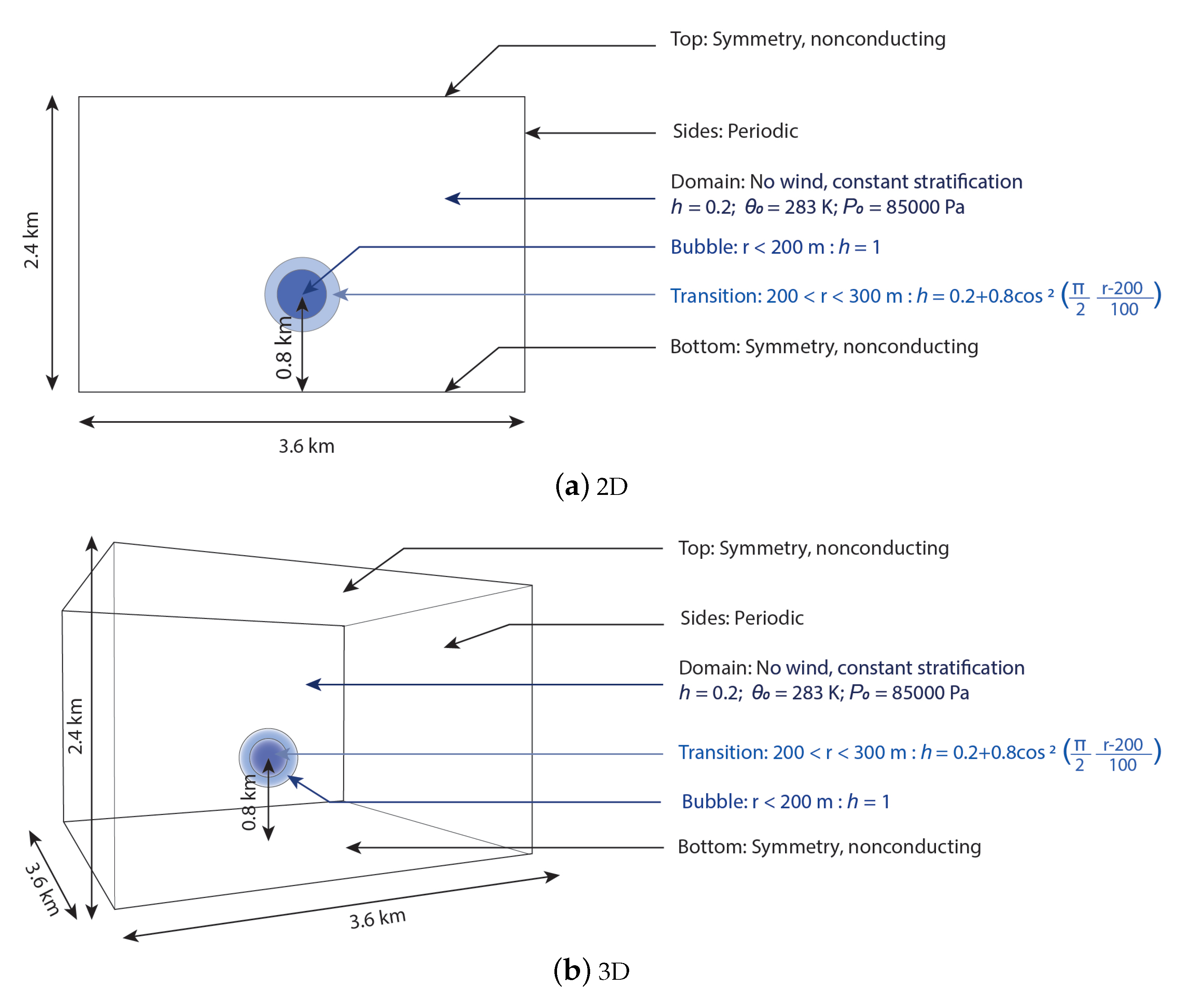
3.2. 2D and 3D Rising Moist Bubbles
The second and third validation cases focus on a 2D and a 3D moist bubbles rising in a 2D or a 3D rectangular domain as shown in Figure 3. In both cases, the domain height was and the domain width was .
In the 2D configuration, a uniform grid with and was used, while in the 3D configuration a nonuniform grid with finest and was considered. Other model settings can be found in Feng et al.’s work [25]. 2D simulations were performed for physical time and the results were compared to reference data at 3, 5 and . 3D simulations were run for physical time and the results were compared to reference data at 2, 4 and .
HRR-LBM simulation results were compared to benchmark solutions, which used a multidimensional positive definitive advection transport algorithm and an anelastic solver with a grid in 2D configuration and on a grid with a finest grid spacing in 3D configuration [28,29].
Regarding the 2D bubble, HRR-LBM and reference results were compared in terms of highest vertical position of the 20% maximum contours and vertical fluid velocity at the top central position of the interface at different times (Table 1). As in the reference study, the HRR-LBM results show the rising and expansion of the moist bubble as the phase changes. HRR-LBM results are thus generally in good agreement with the reference data except for the highest vertical position of the 20% maximum contours and the vertical fluid velocity at the top central position of the interface, especially at , which could be explained by the Boussinesq and not the aneleastic approximation used in the current study.
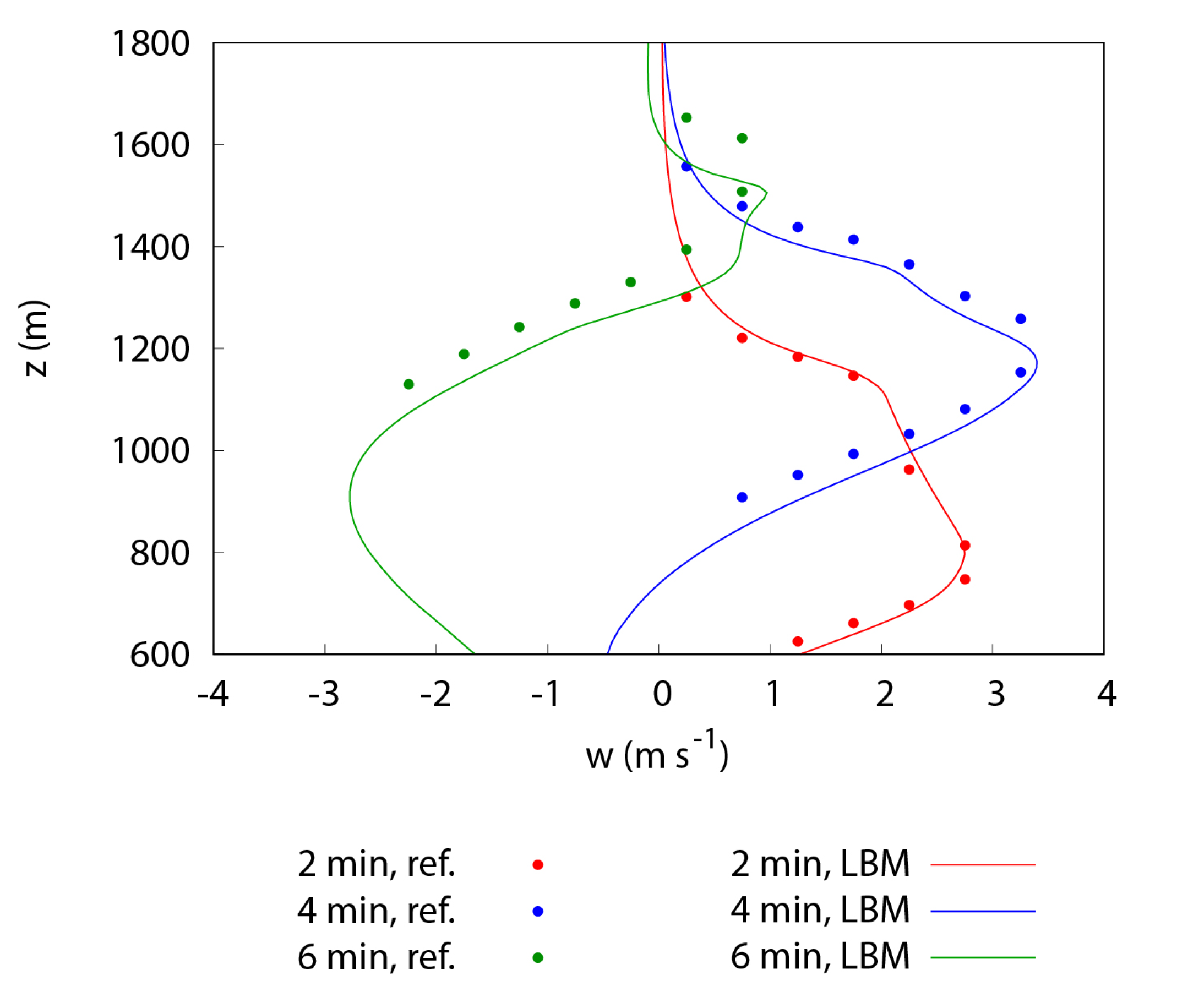
Regarding the 3D case, the good performance of the HRR-LBM model was highlighted by the comparison of the vertical velocity profiles along the midline of the domain (Figure 4) as well as liquid humidity profiles and the liquid and vapour contours (not shown).
3.3. Atmospheric Cloud Formation
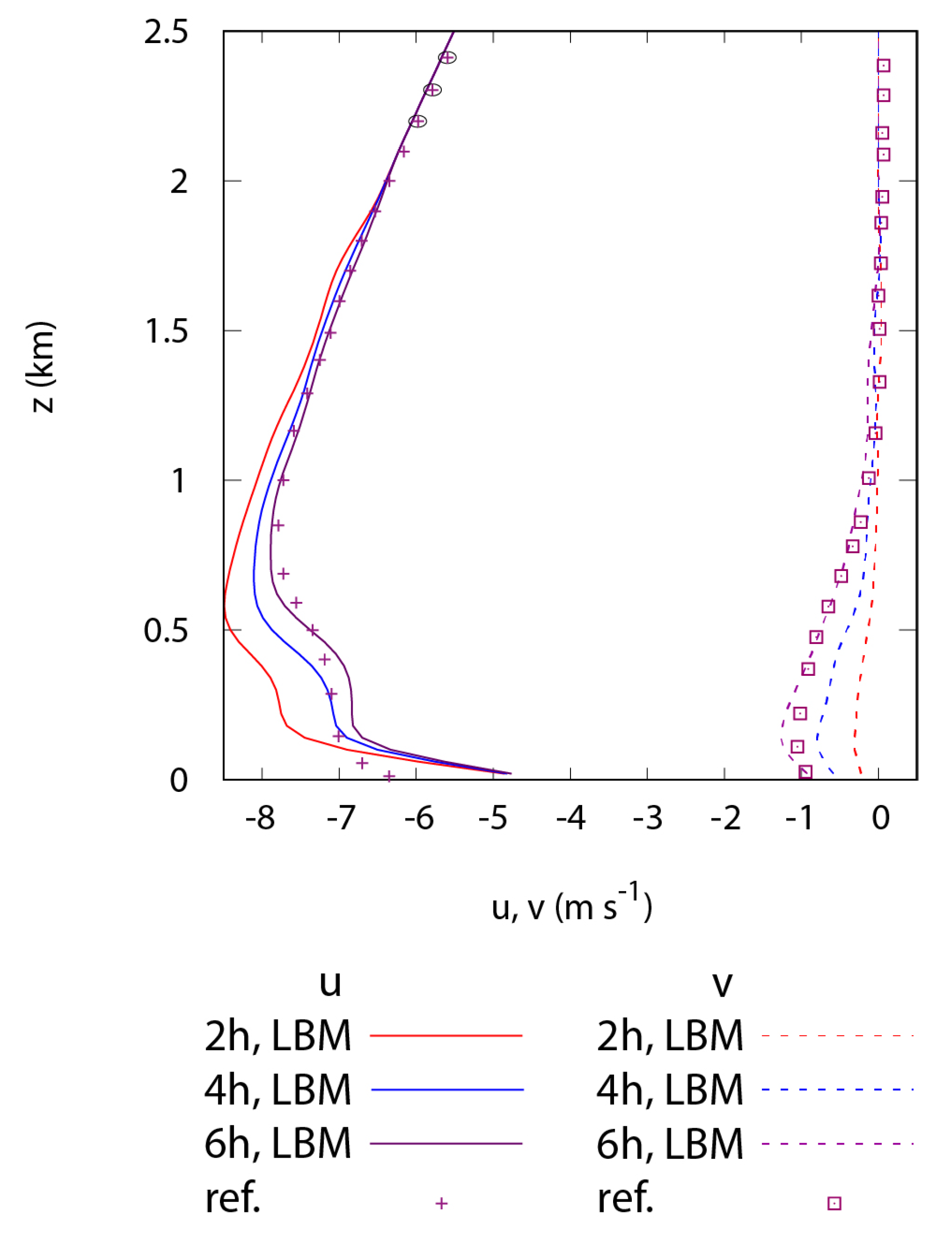
Finally, the fourth validation case addresses a convective atmospheric boundary layer case with a shallow cumulus formation to assess the capability of the HRR-LBM-WMLES model to predict the moist thermodynamics and its interactions with meteorological flows. The configuration refers to the model intercomparison case of the Barbados Oceanographic and meteorological Experiment (BOMEX). The considered domain is a long and high square-based domain with temperature and humidity surface fluxes and underwent an altitude-dependent geostrophic wind. Table 2 gives the related initial conditions.
For this configuration, HRR-LBM-WMLES simulations considered a grid with . The Monin Obukhov similarity theory was used as the surface model of the horizontal momentum components, temperature and humidity, and additional sources terms were added to the model to represent the large scale effects that cannot be included in LES. Details of the model settings can be found in Feng et al.’s work [24,25].
Simulations were run for physical time and statistics were computed on .
The comparison of HRR-LBM and reference results of Siebesma et al. [30] in terms of profiles of mean velocity (Figure 5), potential temperature, vapour and liquid water (not shown) highlights a good performance of the developed HRR-LBM-WMLES model, as the different atmospheric layers (mixed, conditionally unstable and inversion, from the ground upwards) and the instantaneous formation of the cloud are well captured.
Hence, the hybrid LBM-based atmospheric numerical model, including the HRR collision model with forcing terms, and a finite volume method for temperature and water transport equation appear well suited to predict atmospheric humid convection with cloud formation, even considering large scale sources.
4. HRR-LBM-WMLES Application to Urban Pollutant Dispersion
This section reviews different case studies performed to assess the performance and the benefits of the proposed approach regarding the prediction of outdoor urban pollutant dispersion. Geometric complexity (trees, urban patterns) and buoyancy effects (pollutant or thermals) were especially studied.
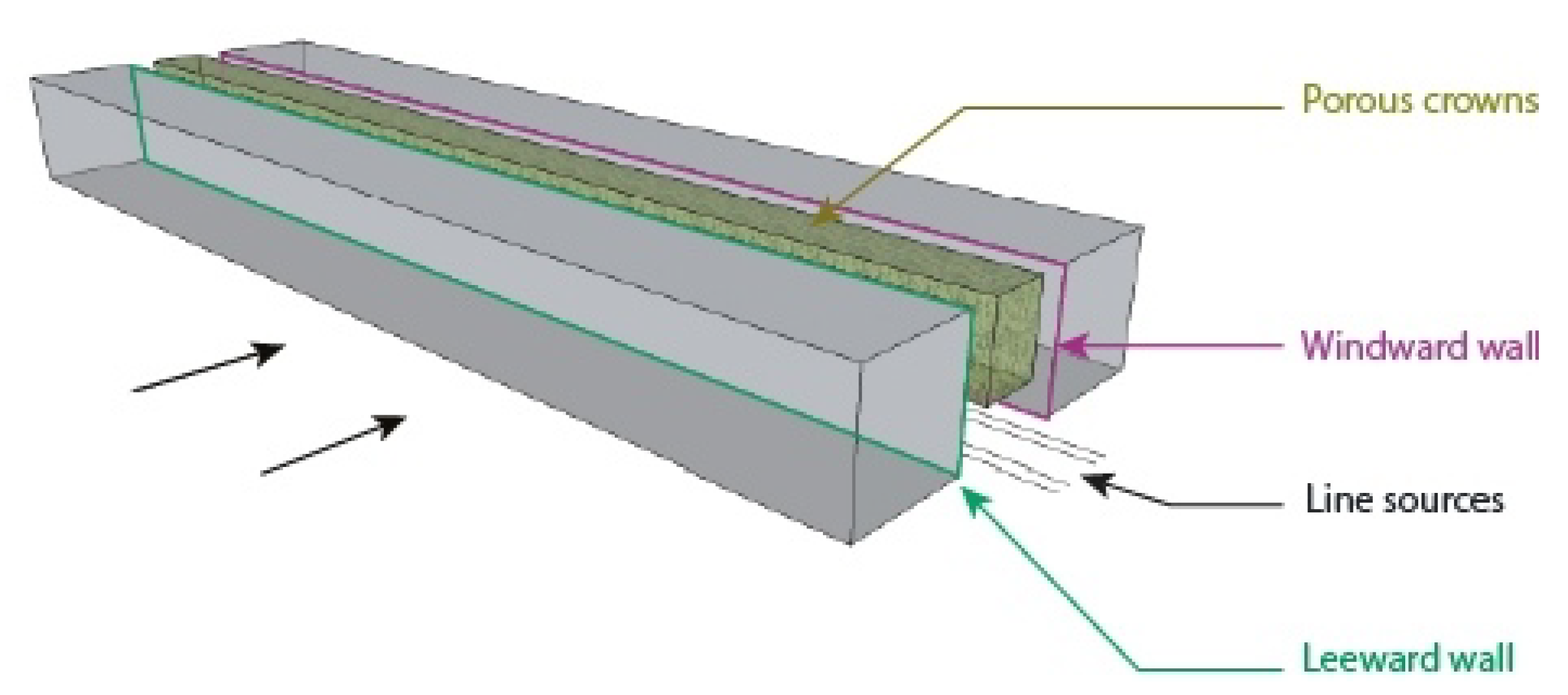
4.1. Dispersion in a Street Canyon Including Tree Planting
A first validation study deals with dispersion of neutral traffic such as pollutant emissions in an ideal street canyon planted or not along a centred row of more or less dense tree crowns ( and , respectively) and undergoing a perpendicular wind (Figure 6).
The drag force () induced by porous media is modeled via a Forchheimmer formulation, as follows:
where is the drag force coefficient and is the ratio of porous media immersed in the volume cell.
Simulations were performed at reduced scale (1:150, ) as in the reference experiment [31], with a domain of and the street canyon located from the inlet. Table 3 gives the different boundary conditions. Accounting for = 0.00125 m, s and five refinement levels, the total number of grid points was . Simulations were run on 240 cores for physical time, with the last being kept for postprocessing. Details can be found in Merlier et al.’s work [32].
Quantitative (Table 4) and qualitative (not shown) comparisons of experimental and numerical mean concentrations on the leeward and windward walls of the street canyon highlight a state of the art performance of the HRR-LB model as compared to other reference studies.
Table 4 especially shows that the global statistical performance indicators generally match the acceptance criteria suggested by Chang and Hanna [33]. Nonetheless, the results show a better agreement between numerical and experimental concentrations on the leeward wall, where the concentration is higher than on the windward wall, and for less dense tree crowns ( and 80 m). The analysis of concentration distributions on walls also highlights higher concentrations on the streamwise symmetry plane as in the reference experiment.
In addition, thanks to high-fidelity unsteady simulations, the analysis of concentration statistics at different locations in the street canyon highlighted that high peaks of concentration can occur notably in the presence of dense tree crowns, which could be particularly harmful for short time exposure problems.
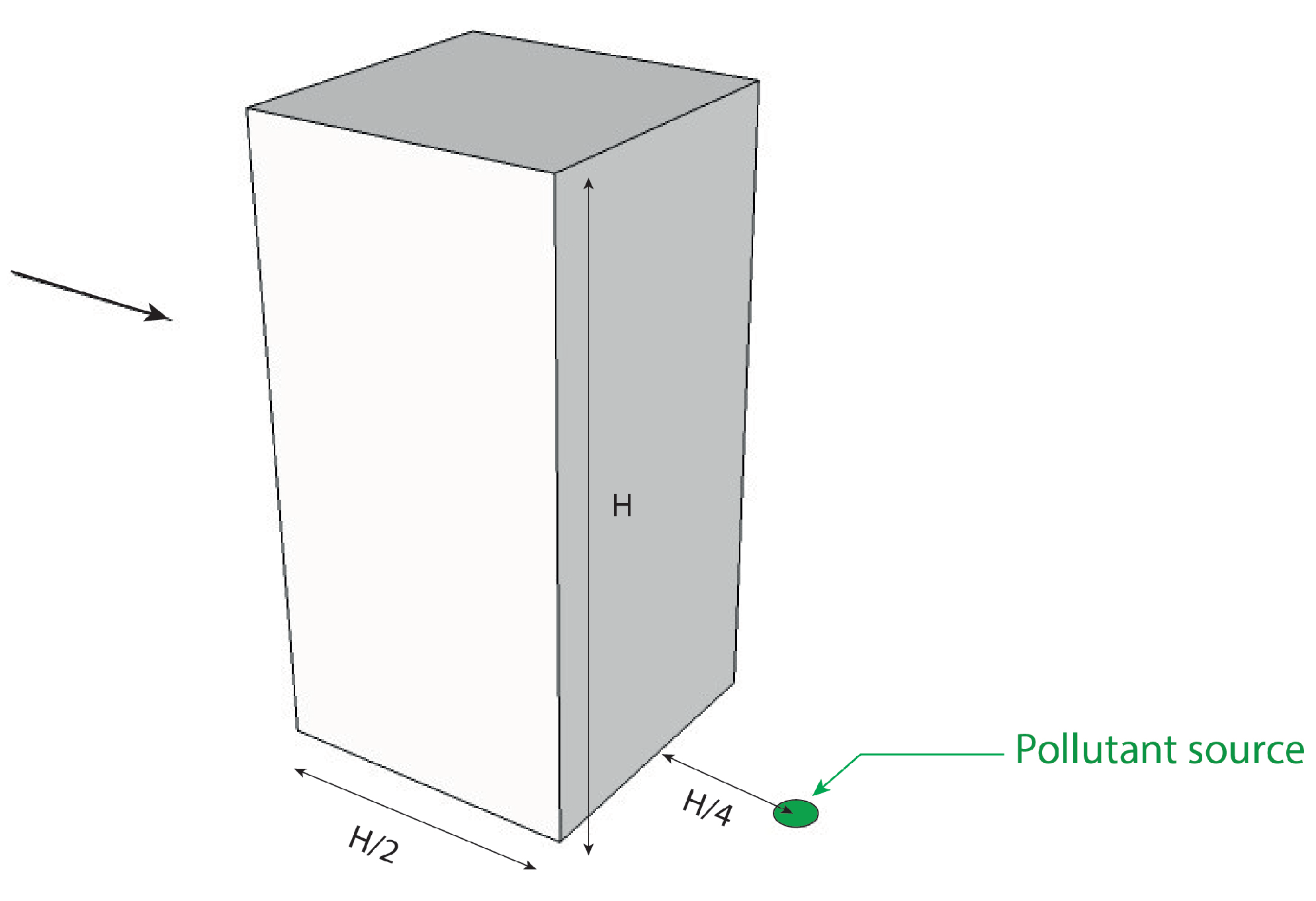
4.2. Dispersion behind a Building under Unstable Stratification
A second validation study deals with the dispersion of a gas released from a ground source just downwind of an isolated building located in an unstable boundary layer (Figure 7).
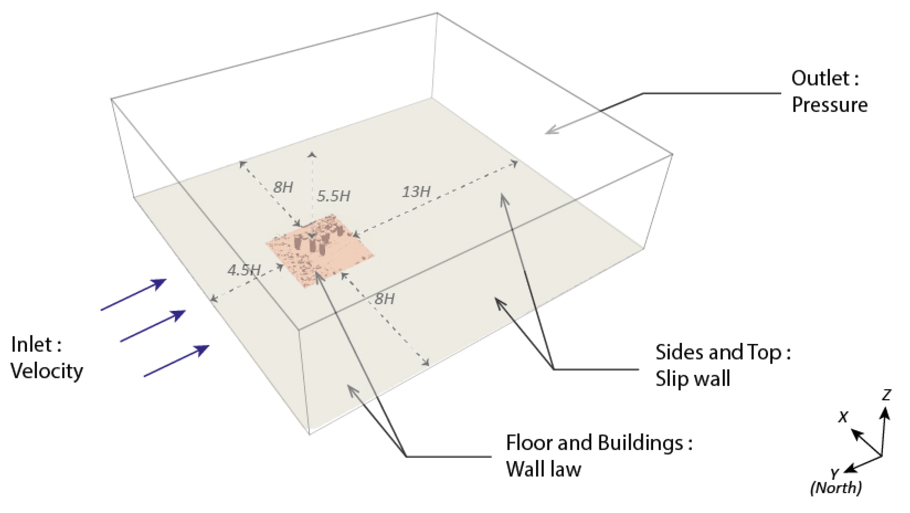
Simulations were performed at a reduced scale () as in the reference study [34], with a domain of according to AIJ guidelines [35], the building being located , and from the inlet, lateral and top domain boundaries, respectively. Table 5 gives the corresponding boundary conditions. Accounting for , s and five refinement levels for the coarse grid case and , s and six refinement levels for the medium grid case, the total number of grid points was for coarse grid and for the medium grid. Simulations were carried out on 28 or 56 cores for physical time, the last being kept to compute the statistics.
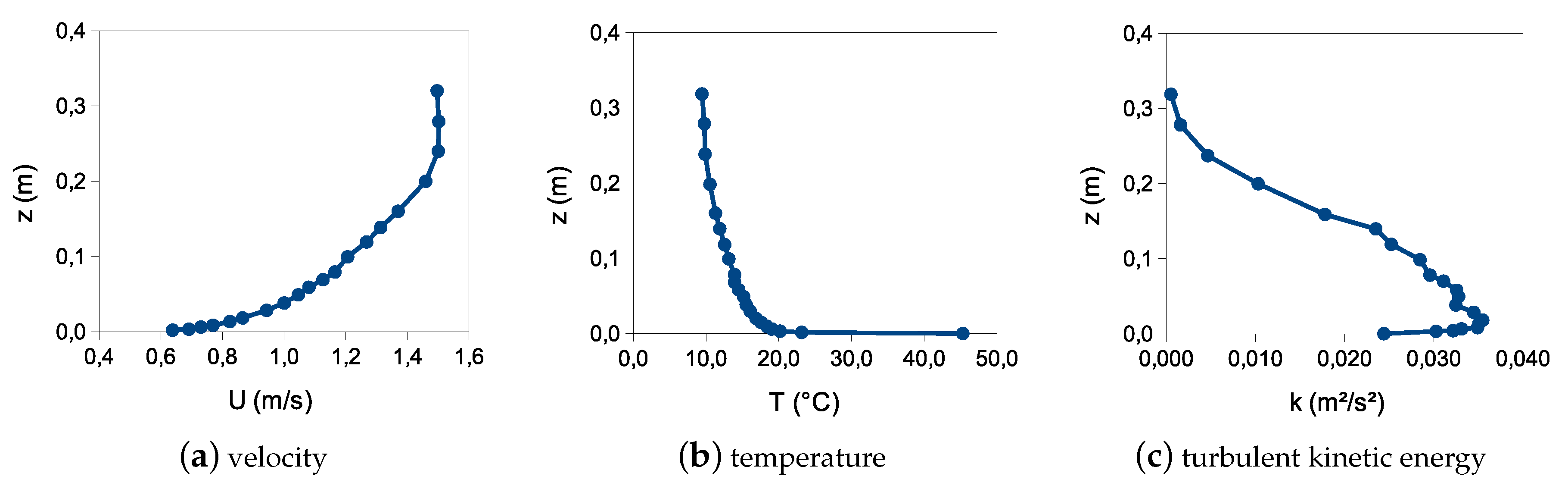
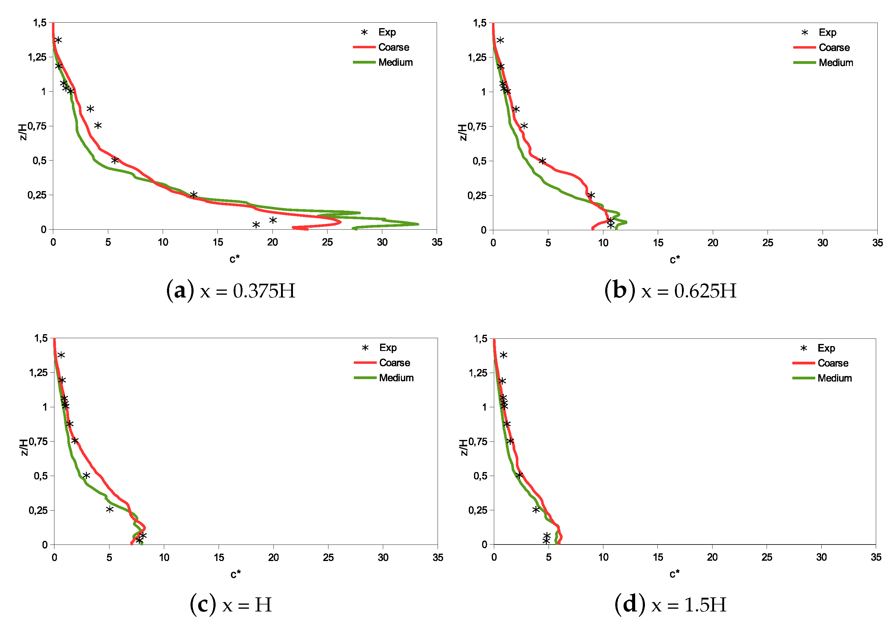
The pollutant source with a diameter of is located downstream the building. A gas flux of with a temperature of was imposed. The inflow velocity, temperature and turbulent kinetic energy were interpolated from experimental data provided in the TPU database [36] and are plotted in Figure 8.
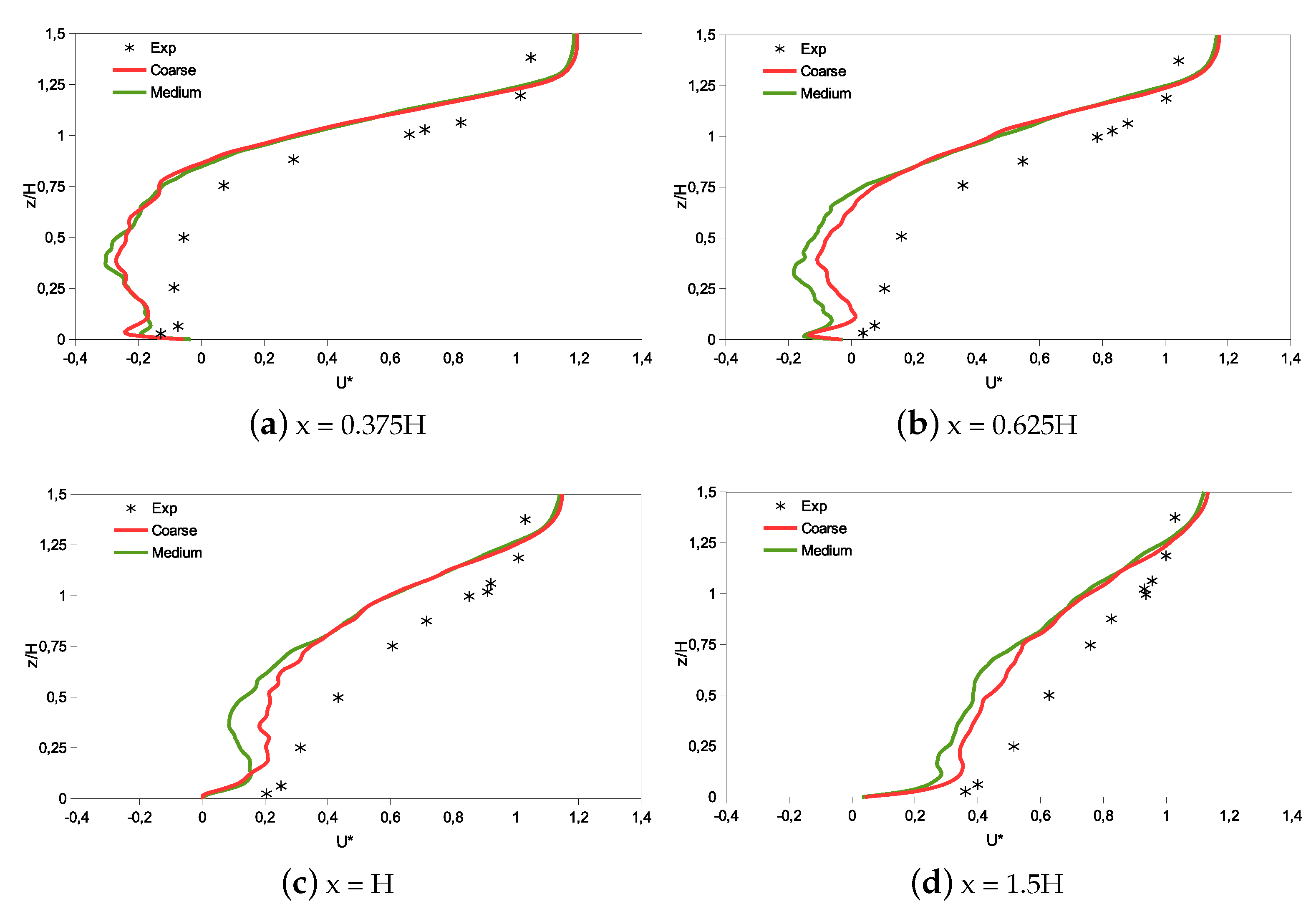
The velocity, temperature and concentration of tracer gas were compared to experimental data at four different locations downstream of the building. Velocity was normalized with the reference velocity at building height (), the temperature was normalized using floor temperature ( and the difference between floor temperature and temperature at building height () and the concentration was normalized by release gas flux, building height and reference velocity ().
Figure 9 and Figure 10 present the comparison of the HRR-LBM results obtained with a coarse and medium grid with the experimental data of Yoshie et al. [37]. A good agreement was obtained for concentration field downstream of the building and the present results are more accurate than other literature LES simulations related to the same case [34,38]. A fairly good agreement was found for streamwise velocity profiles downstream of the building, although velocity is generally underestimated compared to experimental data.
4.3. Dispersion of Neutral and Dense Gas in an Urban Area
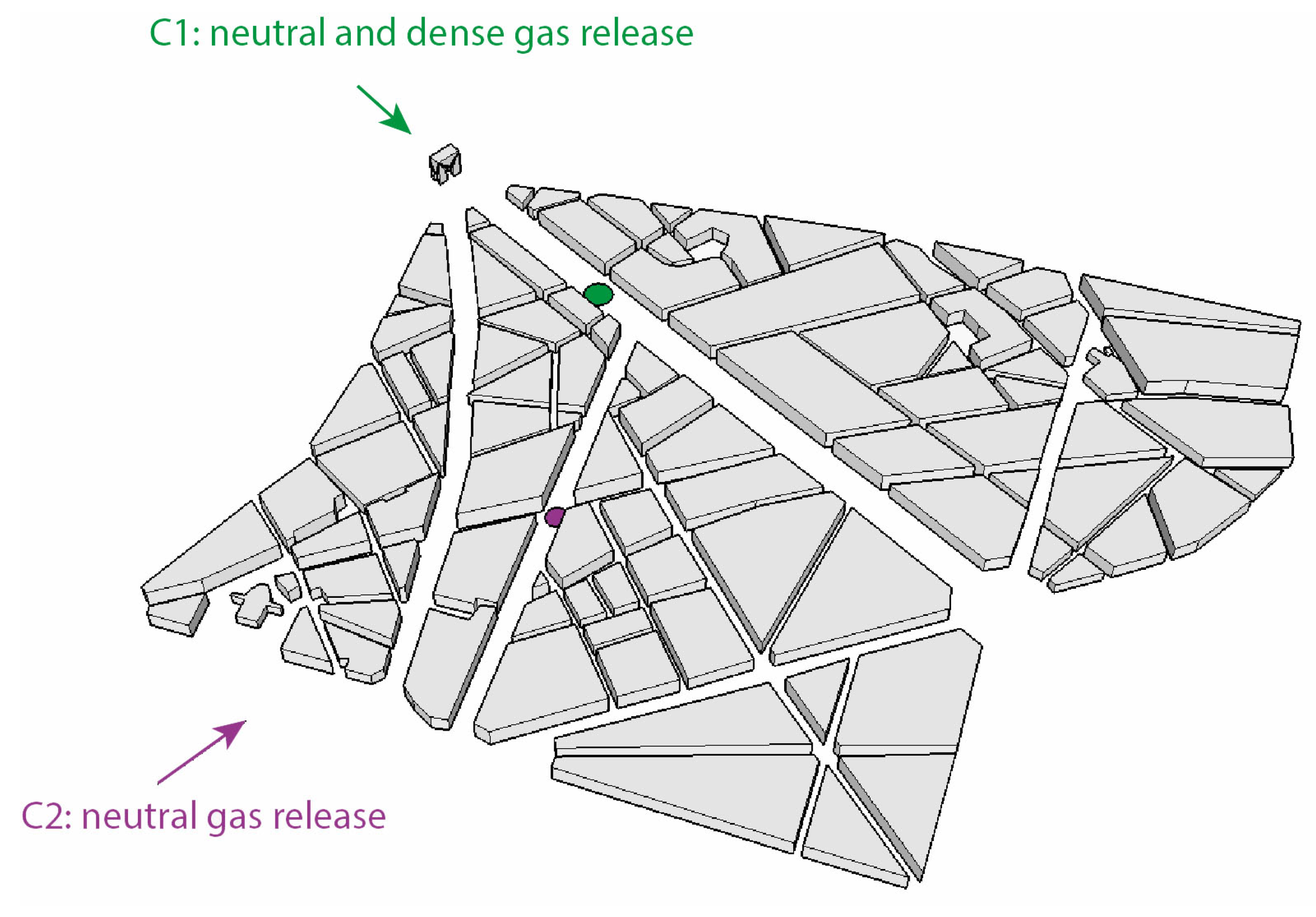
A third validation study deals with the dispersion of neutral and dense gas from a ground source in a realistic urban environment. Two different source locations and wind incidences (C1: neutral and dense gas emitted in a rather channeled flow in a large avenue, C2: neutral gas emitted in a surround built crossroad, see Figure 11) are considered.
Simulations were performed at reduced scale (1:350, ) as in the reference experiment [39], with a domain of 8.75 (C1) or 9.5 (C2) , with the model located from the inlet of the domain. Table 6 gives the different boundary conditions.
Accounting for m and s with six refinement levels, the total number of grid points was (C1) or (C2). Simulations were run on about cores for physical time and statistics were computed over . More details can be found in the work of Merlier et al. [40].
The performance indicators given in Table 7 for concentration at street level highlight a good performance of the model, especially for configuration 2.
Results match the different acceptance criteria for urban dispersion models suggested in the work of Hanna and Chang [41], although the dense gas configuration shows a worse, but still acceptable, accuracy. Indeed, the analysis of the spatial distribution of concentration (not shown) highlights that:
- The neutral gas emitted in the channeled flow is carried mainly in the main street by the prevailing flow and progressively mixes upwards;
- The dense gas emitted in the channeled flow follows a rather circular and flat dispersion all around the source;
- The dispersion of the neutral gas emitted in the crossroad is notably vertical due to the presence of the obstacles built upstream and downstream.
The comparison of the HRR-LBM and reference vertical as well as horizontal concentration profiles above the canopy (not shown) are generally also satisfactory regarding both the mean and the standard deviation of concentration levels. These results suggest that the dynamics of dispersion processes are well reproduced by the model. Being capable of providing the temporal statistics of velocity and concentration, the developed approach appears well suited to support the design of fast response models.
5. HRR-LBM-WMLES-Based Urban Wind Prediction with Application to Pedestrian Wind Comfort and Building Wind Loads under Uncertainty
A next step toward an improved reliability of numerical simulations for realistic full scale urban applications is the capability to account for uncertainties that appear in the prescription of the atmospheric conditions, instantaneous wind conditions, surface roughness, pollutant source features, etc. The variability of the numerical solution with respect to uncertain parameters must be quantified in order to provide users with useful information, since a single fully deterministic solution is meaningless in such problems. To this end, efficient techniques for Uncertainty Quantification (UQ) must be used. A challenging issue is that most existing UQ techniques require the use of a significant number of samples, each sample being currently an unsteady high-fidelity LES of the case under consideration. Therefore, adequate UQ methods must be defined that minimize the number of required simulations while preserving the accuracy of the uncertainty propagation in the results. Such a method, the c-APK method, was developed by Margheri and Sagaut [42] with application to urban flow simulations in complex areas.
The c-APK method will not be detailed here for the sake of brevity, and the reader is referred to Margheri and Sagaut [42] for details. Nonetheless, to highlight two additional applications of the c-APK method, this section reviews two validation studies and two projected applications related to the prediction of urban air flows with UQ: pedestrian wind comfort and wind loads on buildings. The configuration studied for the projected applications is a new hypothetical tower located in a complex and dense urban area.
5.1. Prediction of Mean Flow Field in a Complex Urban Environment
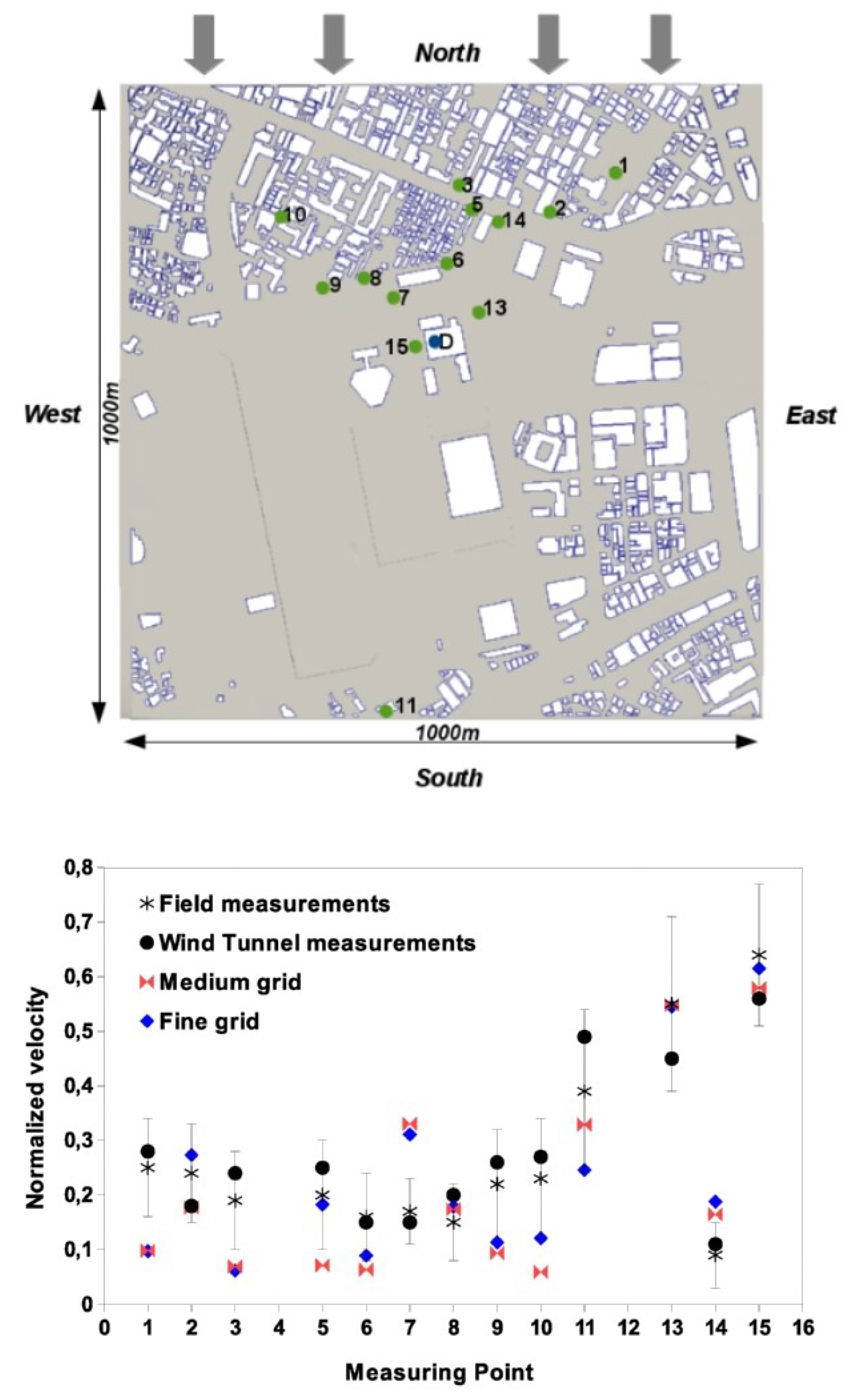
The first validation study focuses on a full scale urban area of Tokyo, which includes an area of low-rise buildings upstream a cluster of towers. Simulations were performed at full scale, considering , to evaluate the performance of the model at a realistic Reynolds number, as both full scale and reduced scale data are provided in the reference experimental data [43]. More precisely, the configuration studied corresponds to the case F of the open source Architectural Institute of Japan’s database, which gathers full scale and wind tunnel measurements, wind tunnel tests corresponding to the 1977 full scale measurements campaign.
Figure 12 details the different model dimensions and boundary conditions used for the simulations.
Accounting for and with seven refinement levels, the total number of grid points was for the finest grid (respectively, , , six refinement levels and grid points for medium grid). Simulations were run on 504 cores (240 for medium grid) for physical time, the last being kept for postprocessing. More details can be found in the work of Jacob and Sagaut [44].
The HRR-LBM and reference mean velocities reported in Figure 13 at high and for different locations in the area of interest evidence a good performance of the developed model and also for mean velocity.
5.2. Prediction of Surface Pressure on a High-Rise Building
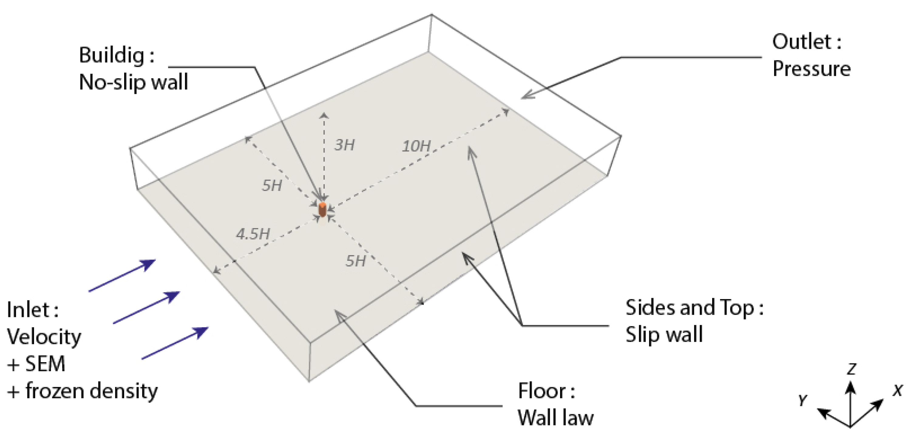
To evaluate the accuracy of the developed approach also on building surface quantities before coupling the HRR-LBM-WMLES tool with a UQ technique, a second validation study was extensively carried out at a reduced scale isolated high-rise building (1:300, ), for which detailed measurement data of velocity and pressure on the model surface are available [45]. Figure 14 details the different model dimensions and boundary conditions, which included an extension of the original incompressible SEM to reconstruct the inlet turbulence in the current LBM framework, given the importance of the turbulent inflow properties dynamically studying wind loading on isolated structures.
With m and s and six refinement levels, the total number of grid points was . More details can be found in the work of Buffa et al. [23].
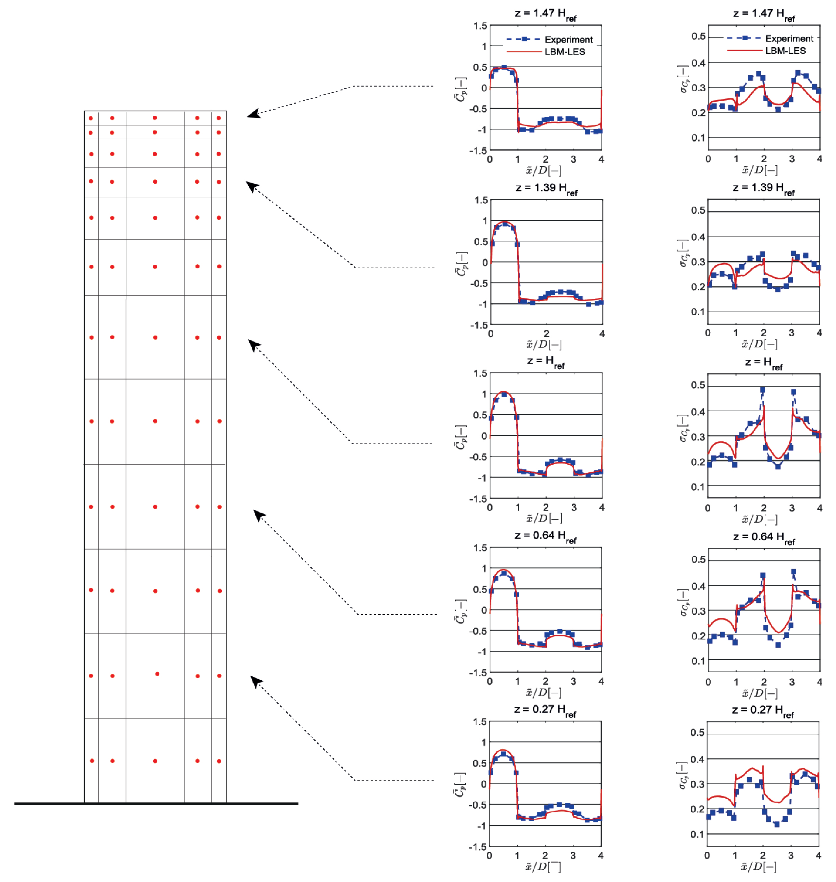
The comparison of mean and standard deviation values of pressure coefficients at the building surface for the different faces of the building and at different heights (Figure 15) shows a very satisfactory match for all the tested data, especially for the mean value. Experimental and simulated data were also extensively compared in terms of spectral analysis and local instantaneous pressure maxima (not shown), showing the reliability of the developed approach for wind load prediction.
5.3. Wind Comfort Assessment with Uncertainty Quantification
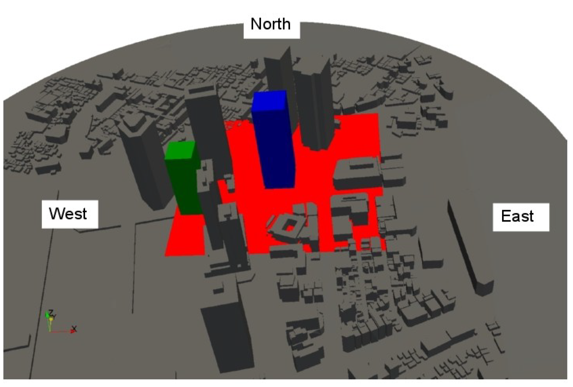
Thanks to the possibilities offered by the developed dynamic model, pedestrian wind comfort at street level () was studied considering Melbourne criteria [46] in an area of inside Shinjuku area as shown in red in Figure 16.
The domain used in this study is the same as in Section 5.1. Simulations were run on physical time and the statistics were computed over the last hour. As described by Jacob and Sagaut [44], two buildings were added in Shinjuku area: one in the middle of the area (in blue in Figure 16) for wind comfort assessment and one (in green in Figure 16) for the study of Section 5.4. The case presented by Jacob and Sagaut [44] with the wind coming from the north is here considered as the reference sample for the UQ analysis, and several other samples have been considered by changing the velocity magnitude by a factor () and wind direction with an angle around the north direction (). A set of 57 simulations have been performed for this study permitting to estimate first the sensitivity of the mean velocity field to and and to compute the mean value of mean velocity at pedestrian level using the c-APK method.
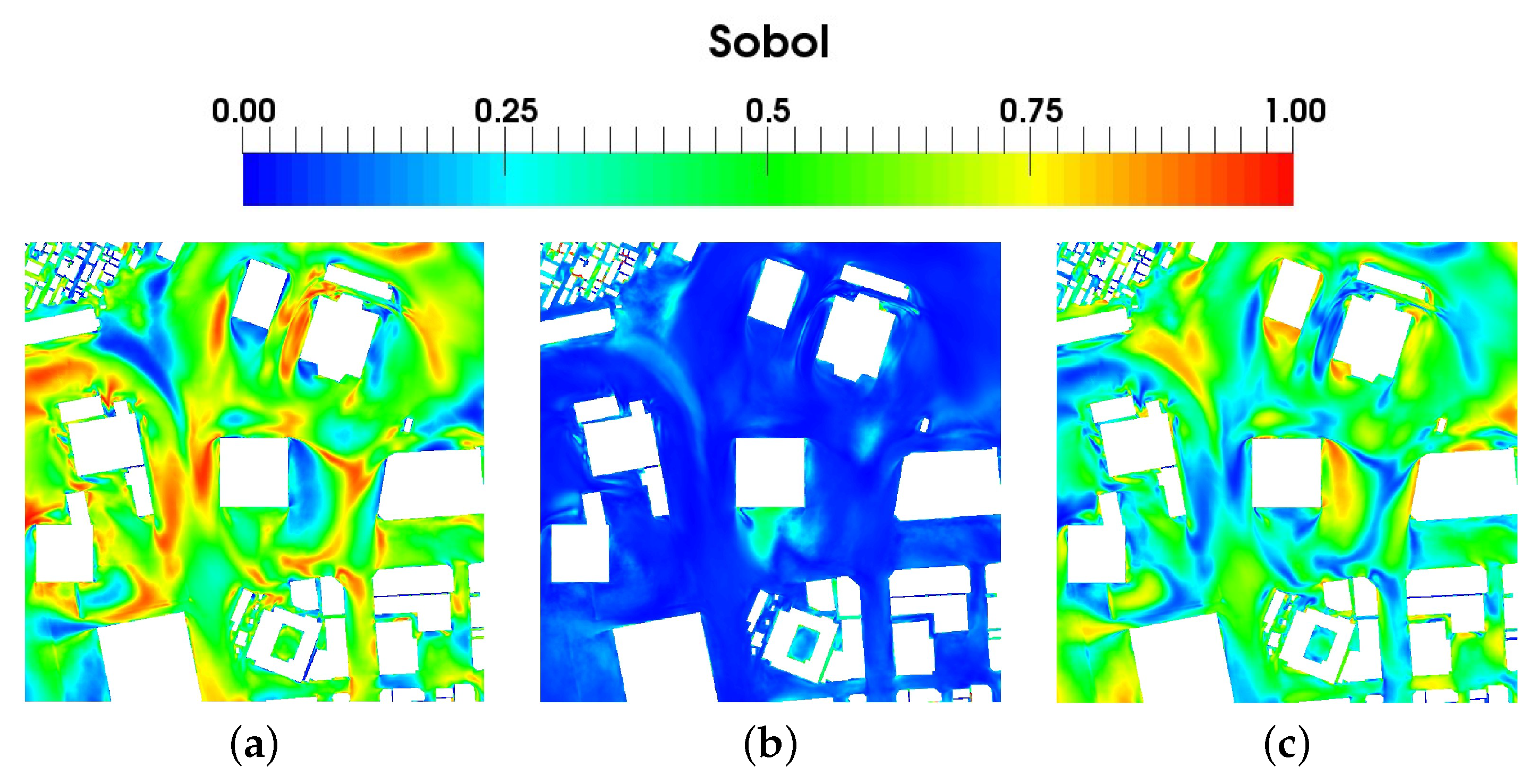
Figure 17 shows the Sobol indices obtained for the mean velocity field at the pedestrian level, which permits quantification the influence of each parameter on the global variance of the system. The results highlight that the inflow velocity magnitude is generally the main influential parameter in most locations in the area of interest. In some locations, wind direction has a large contribution on the variance, especially in areas that can be located in wake for some inflow directions.
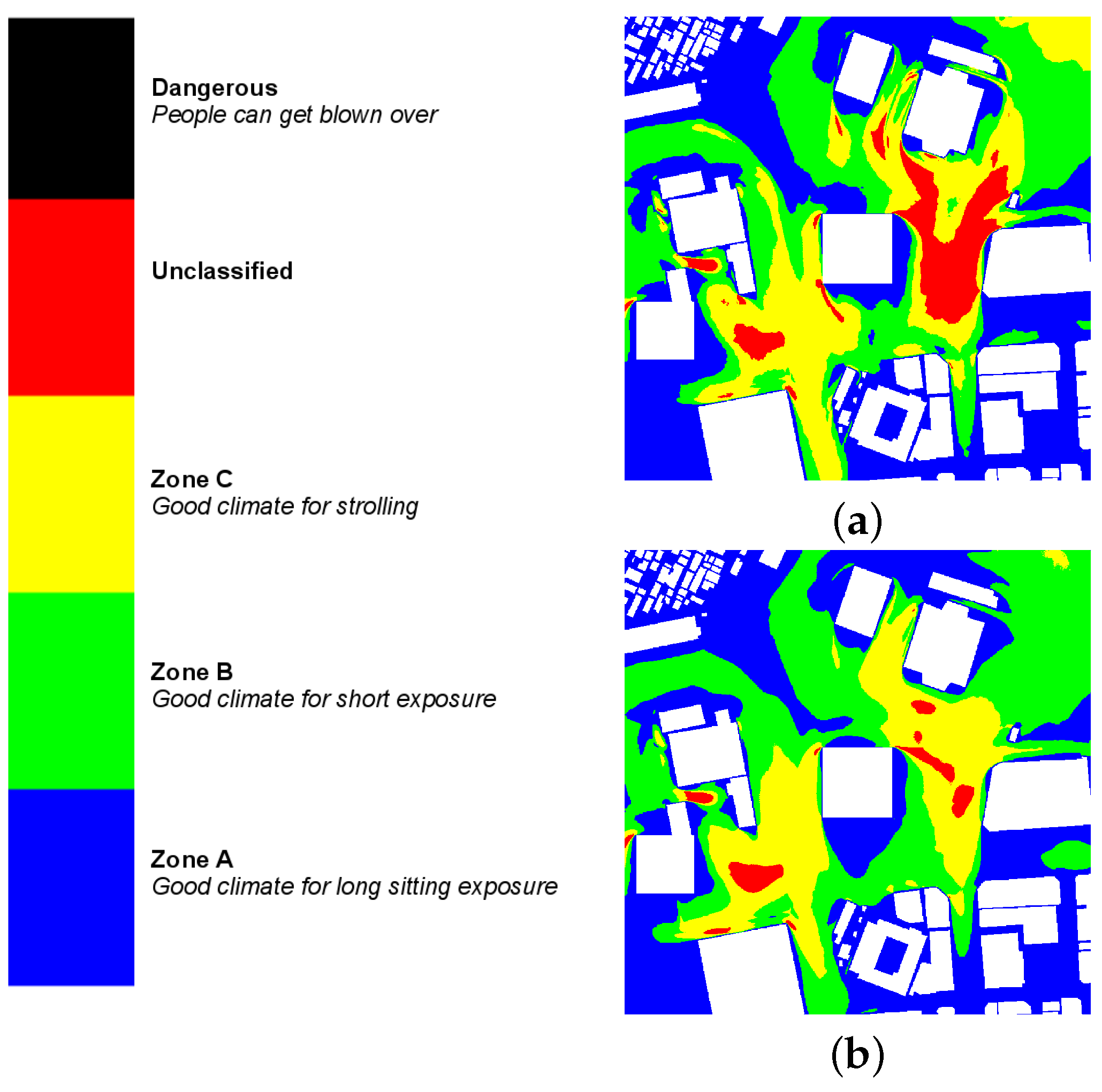
Figure 18 shows the classification obtained following the Melbourne criteria using the data of the reference sample (, ) and the mean data obtained from the 57 samples. The results highlight that by using the c-APK output, a large part of the area is located in Zones A, B and C where pedestrian comfort can be considered as good, whereas a part of the area is unclassified (here the pedestrian comfort is not so good) using only the reference sample.
5.4. Prediction of Structural Wind Loads with Uncertainty Quantification
The same configuration as in Section 5.3 was considered to study pressure distribution on the facades of the hypothetical building (green building in Figure 16) for further applications to the prediction of structural wind loads. The analysis is based on the same set of simulations changing the inflow velocity magnitude and direction.
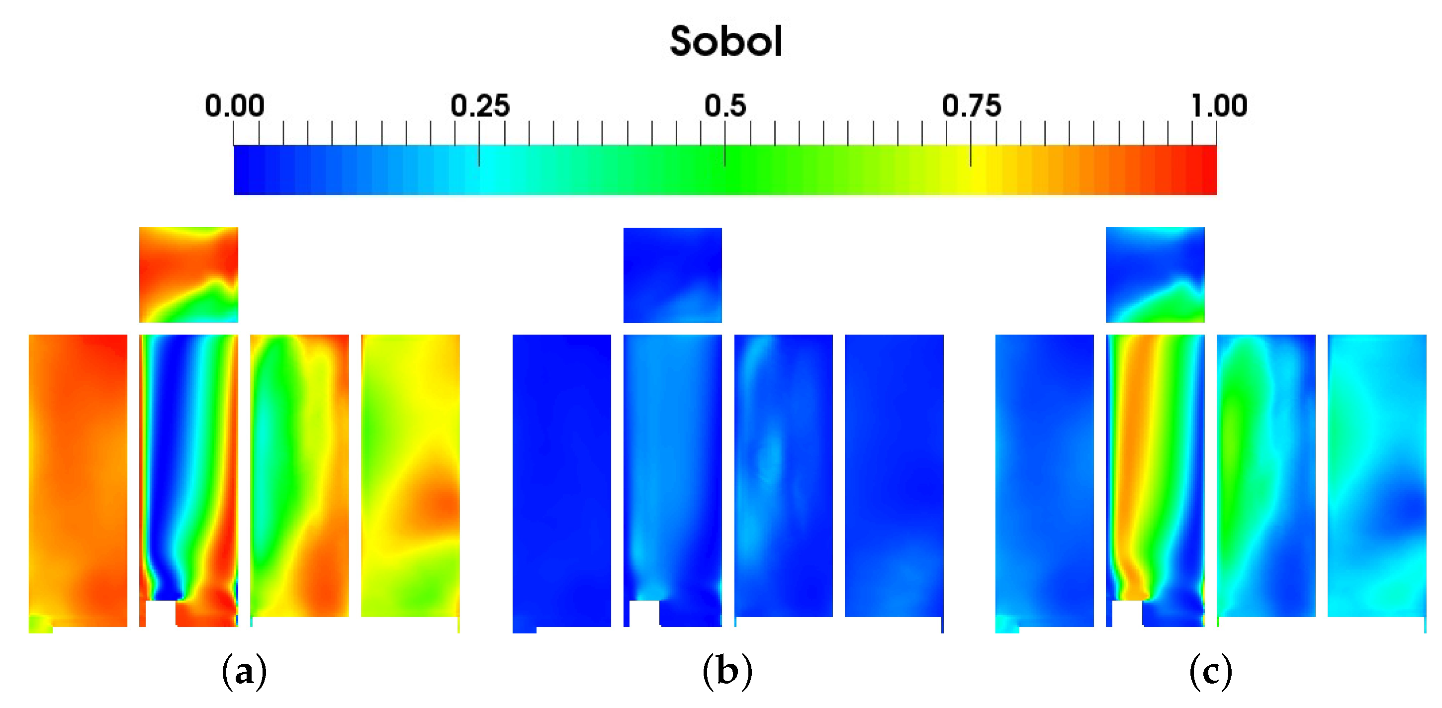
The Sobol indices plotted on the different building faces in Figure 19 highlight that the inflow velocity magnitude is the most influential parameter on the pressure distribution on the building faces, except on a part of the north face, where the wind direction appears to influence pressure values more than the wind velocity magnitude.
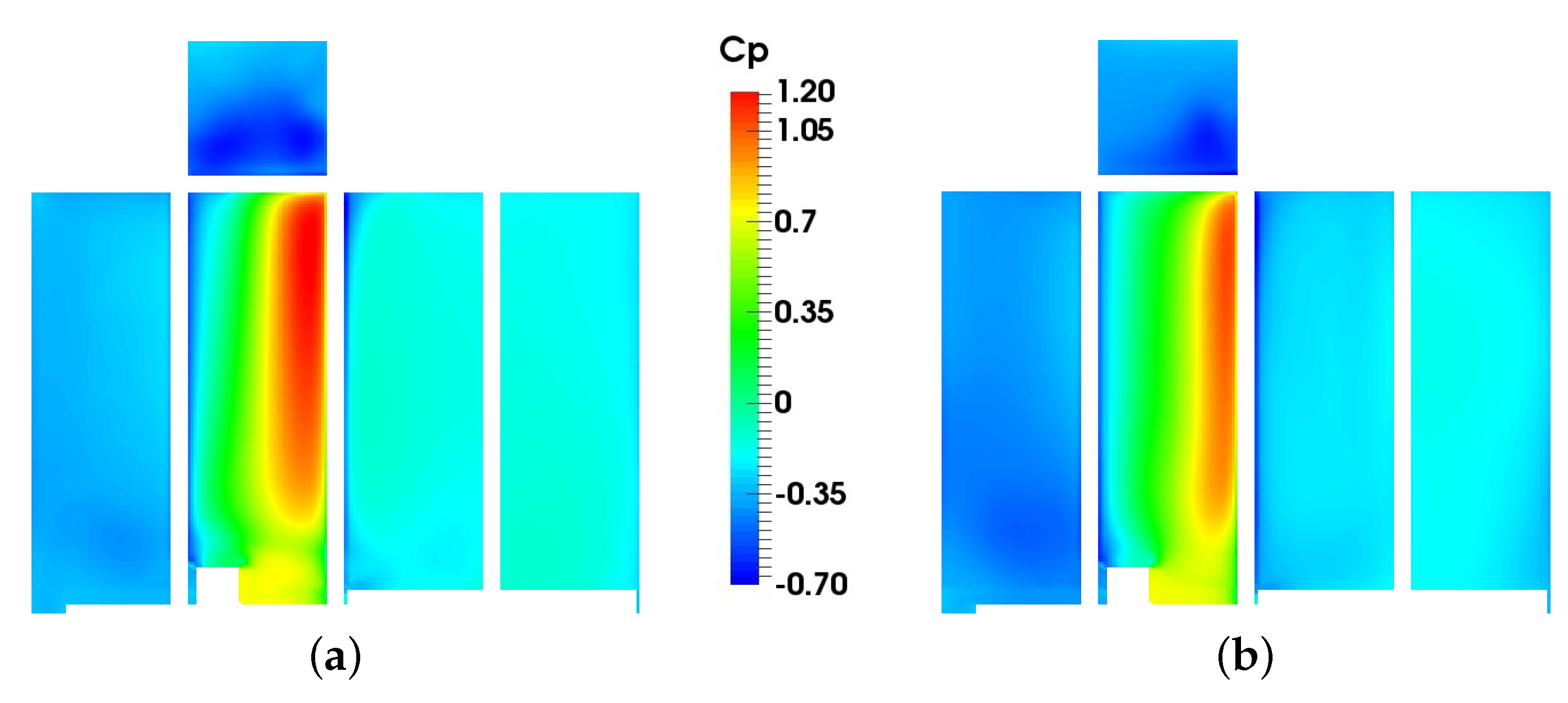
This is explained by the fact that a large part of the north face is located in a wake area when the flow is coming from the northeast direction, whereas it is directly exposed to inflow wind when it comes from the northwest direction. The second order term is very low compared to the others and does not significantly contribute to the global variance of the pressure on building faces. Figure 20 presents the pressure coefficients obtained in the case of the reference sample (, ) on the different building faces and the pressure coefficients computed from the average pressure given by the c-APK analysis. Few differences were observed on top, east, west and south faces, whereas the estimated pressure coefficient was lowered by the c-APK analysis on the north face compared to the reference sample.
This result suggests that uncertainties on the inflow wind should be accounted for in urban simulations since it has an impact on the dynamics of the flow around high-rise buildings and on the related surface quantities.
6. Indoor Pollutant Dispersion with Thermal and Moving Body Effects
Another step toward the numerical simulation of realistic full scale configuration is the use of high-fidelity CFD for evacuation problems. In such cases, human agents present in the domain under consideration may have an effect on the pollutant dispersion because they trigger some physical mechanisms (mixing induced by the wakes of moving persons, natural convection due to the heat release by persons, breathing effects, etc.), leading to the definition of a two-way coupling problem. In such a problem, the behaviour of human agents has a direct influence on the flow, but it is governed by their responses to external parameters, which result from the conjunction of physical (e.g., heat) and psychological parameters. Therefore, a more complex level of modeling is required that couples classical physical CFD to psychological and behavioural models.
The present HRR-LBM-WMLES model has been coupled with a Social Force Model (SFM) [47,48,49,50] that allows us to evaluate individual human displacement, taking into account some psychological effects, and therefore to account for the effect of crowd evacuation on pollutant dispersion. The trajectories of people leaving a room are evaluated using SFM, then the drag force of each person is added into LBM equation using the actuator line method (ALM) [51] to account for the effect of human motion on the fluid, leading to the occurrence of wakes.
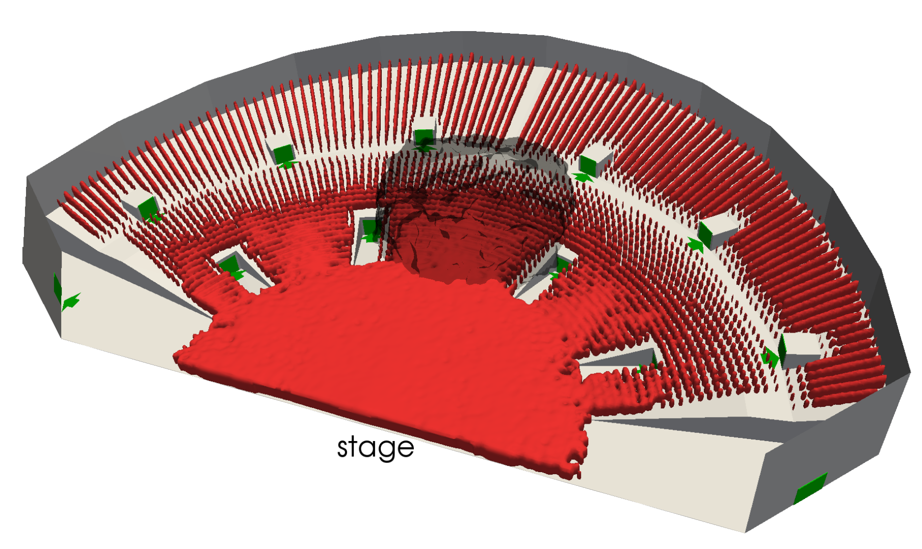
An application of this coupled method is shown here. It is related to an evacuation scenario inside a concert hall [52]. This hall (with dimensions ) contains 12 exits, indicated in green in Figure 21, and is initially occupied by 6026 persons. The concert hall is equipped with ventilation systems located on the room ceiling that allow for the balancing of the heat release of the persons in the concert hall.
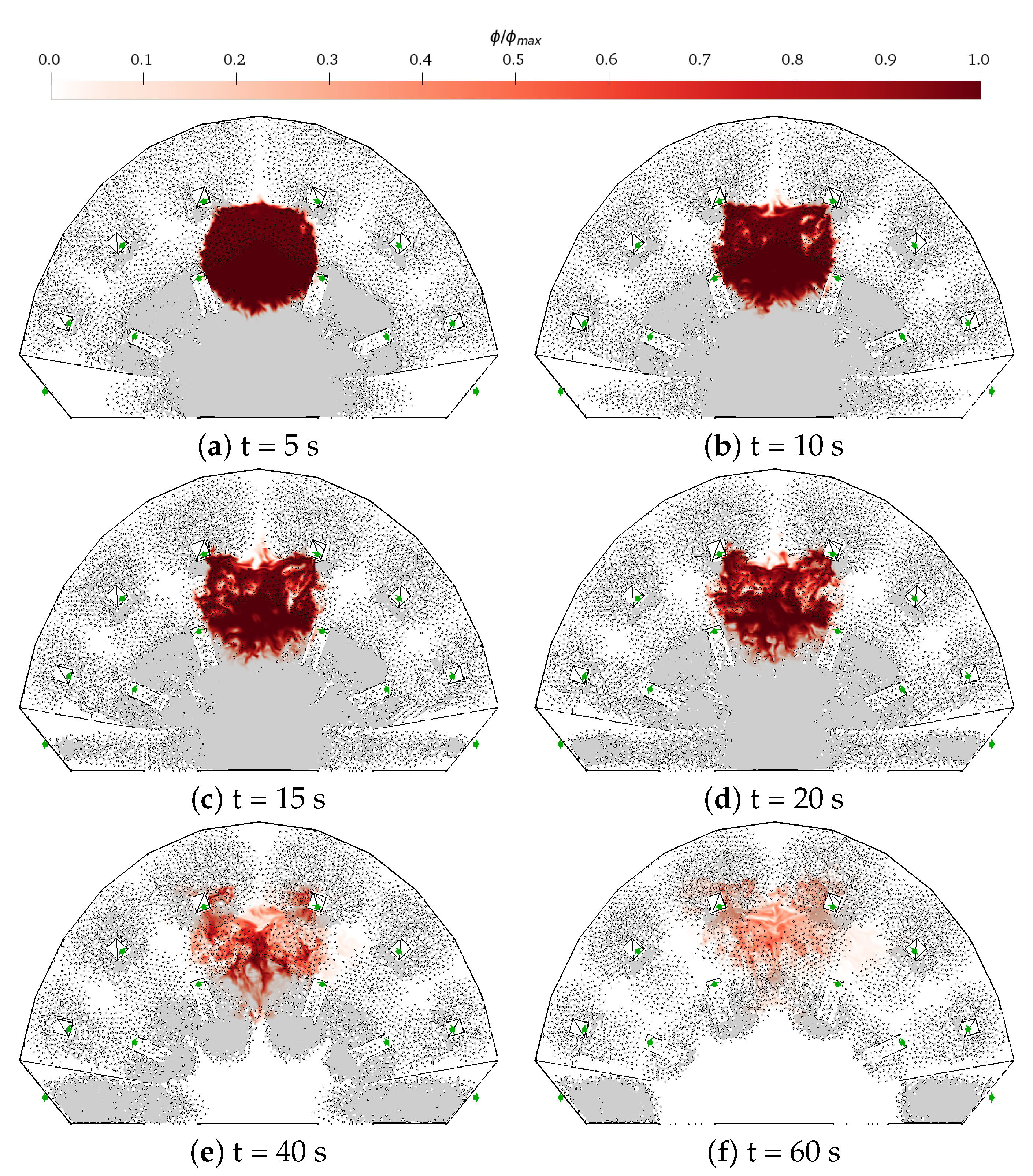
We consider an instantaneous pollutant release from a cloud with a diameter in the centre of the concert hall, as shown in Figure 21. Evacuation starts at the same time as pollutant release and are necessary to allow all the people inside the concert hall to exit.
The pollutant field at human head level obtained at several times is displayed in Figure 22. We can see here that the pollutant is advected inside persons wake from the initial cloud to the two central upper exits. Pollutant dispersion towards the other exits is not significant since people leaving the concert all through these exits were not initially located inside the cloud.
7. Concluding Remarks
The versatility and efficiency of the HRR-LBM-WMLES approach for atmospheric flow simulations, urban physics and pollutant transport prediction have been illustrated by a broad range of applications including humidity effects with phase changes and evacuation prediction with coupling to a social force model.
The main advantages of the present approach are its efficiency in terms of computational time, which is due to the explicit nature of the lattice Boltzmann method, the compactness of the underlying stencil, and the preprocessing time which is drastically reduced thanks to the use of embedded uniform grids along with an immersed boundary approach to handle complex fully arbitrary geometries.
In all cases, a very satisfactory agreement with reference data (if they exist) is reported, demonstrating the accuracy of the simulation tool. The coupling with the c-APK method for uncertainty quantification was also illustrated, showing that the HRR-LBM-WMLES tool is fast enough to allow for the use of UQ tools in complex full scale configurations.
Hence, thanks to its reliability—highlighted through the different validation studies—relevance—highlighted by the different physical analyses carried out—and its computational efficiency—induced by its numerical properties—the developed method appears very to be promising to support the design of fast response models and urban decision making.
Author Contributions
Conceptualization, J.J., L.M., F.M. and P.S.; methodology, J.J., L.M., F.M. and P.S.; software, J.J.; validation, J.J., L.M. and F.M.; formal analysis, J.J., L.M. and F.M.; writing—original draft preparation, J.J. and L.M.; writing—review and editing, F.M. and P.S.; supervision, P.S.; project administration, P.S. All authors have read and agreed to the published version of the manuscript.
Funding
This research received no external funding.
Institutional Review Board Statement
Not applicable.
Informed Consent Statement
Not applicable.
Data Availability Statement
Not applicable.
Acknowledgments
Centre de Calcul Intensif d’Aix-Marseille is acknowledged for granting access to its high-performance computing resources. This work was granted access to the HPC resources of TGCC/CINES under the allocation 2021-A0092A07679 made by GENCI.
Conflicts of Interest
The authors declare no conflict of interest.
Abbreviations
The following abbreviations are used in this manuscript:
| CFD | Computational Fluid Dynamics |
| LES | Large Eddy Simulation |
| LBM | Lattice Boltzmann Method |
| SEM | Synthetic Eddy Method |
| BGK | Bhatnagar Gross Krook |
| MRT | Multiple Relaxation Time |
| HRR | Hybrid Recursive Regularized |
| WMLES | Wall Model Large Eddy Simulation |
| QUICK | Quadratic Upstream Interpolated Scheme for Convective Kinematic |
| c-APK | centered Anova POD Kriging |
| UQ | Uncertainty Quantification |
| NS | Navier Stokes |
| ALM | Actuator Line Model |
References
- Schlünzen, K.H.; Grawe, D.; Bohnenstengel, S.I.; Schlüter, I.; Koppmann, R. Joint modelling of obstacle induced and mesoscale changes—Current limits and challenges. J. Wind Eng. Ind. Aerodyn. 2011, 99, 217–225. [Google Scholar] [CrossRef]
- Sagaut, P. Large Eddy Simulation for Incompressible Flows: An Introduction; Springer Science & Business Media: Berlin/Heidelberg, Germany, 2006. [Google Scholar]
- Blocken, B. 50 years of Computational Wind Engineering: Past, present and future. J. Wind Eng. Ind. Aerodyn. 2014, 129, 69–102. [Google Scholar] [CrossRef]
- Blocken, B. LES over RANS in building simulation for outdoor and indoor applications: A foregone conclusion? In Building Simulation; Springer: Berlin/Heidelberg, Germany, 2018. [Google Scholar]
- Krüger, T.; Kusumaatmaja, H.; Kuzmin, A.; Shardt, O.; Silva, G.; Viggen, E. The Lattice Boltzmann Method. Principles and Practice; Springer: Berlin/Heidelberg, Germany, 2017. [Google Scholar]
- Chen, S.; Doolen, G.D. Lattice Boltzmann method for fluid flows. Annu. Rev. Fluid Mech. 1998, 30, 329–364. [Google Scholar] [CrossRef] [Green Version]
- Slotnick, J.; Khodadoust, A.; Alonse, J.; Darmofal, D.; Gropp, W.; Lurie, E.; Mavriplis, D. CFD Vision 2030 study: A path revolutionnary computational aerosciences. NASA-CR 2014, 2014, 218178. [Google Scholar]
- Ahmad, N.H.; Inagaki, A.; Kanda, M.; Onodera, N.; Aoki, T. Large-eddy simulation of the gust index in an urban area using the lattice Boltzmann method. Bound.-Layer Meteorol. 2017, 163, 447–467. [Google Scholar] [CrossRef]
- Inagaki, A.; Kanda, M.; Ahmad, N.H.; Yagi, A.; Onodera, N.; Aoki, T. A numerical study of turbulence statistics and the structure of a spatially-developing boundary layer over a realistic urban geometry. Bound.-Layer Meteorol. 2017, 164, 161–181. [Google Scholar] [CrossRef]
- Lenz, S.; Schönherr, M.; Geier, M.; Krafczyk, M.; Pasquali, A.; Christen, A.; Giometto, M. Towards real-time simulation of turbulent air flow over a resolved urban canopy using the cumulant lattice Boltzmann method on a GPGPU. J. Wind Eng. Ind. Aerodyn. 2019, 189, 151–162. [Google Scholar] [CrossRef]
- Onodera, N.; Idomura, Y.; Hasegawa, Y.; Nakayama, H.; Shimokawabe, T.; Aoki, T. Real-Time Tracer Dispersion Simulations in Oklahoma City Using the Locally Mesh-Refined Lattice Boltzmann Method. Bound.-Layer Meteorol. 2021, 179, 187–208. [Google Scholar] [CrossRef]
- King, M.F.; Khan, A.; Noakes, C. Coupled indoor/outdoor airflow simulation comparing ANSYS Fluent with a GPU-based lattice Boltzmann model for urban environments. In Proceedings of the Indoor Air 2015, Philadelphia, PA, USA, 22 July 2018. [Google Scholar]
- King, M.F.; Khan, A.; Delbosc, N.; Gough, H.L.; Halios, C.; Barlow, J.F.; Noakes, C.J. Modelling urban airflow and natural ventilation using a GPU-based lattice-Boltzmann method. Build. Environ. 2017, 125, 273–284. [Google Scholar] [CrossRef]
- CS. ProLB. 2021. Available online: http://www.prolb-cfd.com/ (accessed on 28 May 2021).
- M2P2. LaBS. 2021. Available online: http://www.m2p2.fr/valorisation-6/transfert-technologique-labs-3202.htm (accessed on 28 May 2021).
- Wilhelm, S.; Jacob, J.; Sagaut, P. An explicit power-law-based wall model for lattice Boltzmann method—Reynolds-averaged numerical simulations of the flow around airfoils. Phys. Fluids 2018, 30, 065111. [Google Scholar] [CrossRef] [Green Version]
- Wilhelm, S.; Jacob, J.; Sagaut, P. A new explicit algebraic wall model for LES of turbulent flows under adverse pressure gradient. Flow Turbul. Combust. 2021, 106, 1–35. [Google Scholar] [CrossRef]
- Cai, S.G.; Degrigny, J.; Boussuge, J.F.; Sagaut, P. Coupling of turbulence wall models and immersed boundaries on Cartesian grids. J. Comput. Phys. 2021, 429, 109995. [Google Scholar] [CrossRef]
- Jacob, J.; Malaspinas, O.; Sagaut, P. A new hybrid recursive regularised Bhatnagar–Gross–Krook collision model for Lattice Boltzmann method-based large eddy simulation. J. Turbul. 2018, 19, 1051–1076. [Google Scholar] [CrossRef] [Green Version]
- Guo, Z.; Zheng, C.; Shi, B. Discrete lattice effects on the forcing term in the lattice Boltzmann method. Phys. Rev. E 2002, 65, 046308. [Google Scholar] [CrossRef]
- Feng, Y.; Guo, S.; Jacob, J.; Sagaut, P. Solid wall and open boundary conditions in hybrid recursive regularized lattice Boltzmann method for compressible flows. Phys. Fluids 2019, 31, 126103. [Google Scholar]
- Jarrin, N.; Benhamadouche, S.; Laurence, D.; Prosser, R. A synthetic-eddy-method for generating inflow conditions for large-eddy simulations. Int. J. Heat Fluid Flow 2006, 27, 585–593. [Google Scholar] [CrossRef] [Green Version]
- Buffa, E.; Jacob, J.; Sagaut, P. Lattice-Boltzmann-based large-eddy simulation of high-rise building aerodynamics with inlet turbulence reconstruction. J. Wind Eng. Ind. Aerodyn. 2021, 212, 104560. [Google Scholar] [CrossRef]
- Feng, Y.; Miranda-Fuentes, J.; Guo, S.; Jacob, J.; Sagaut, P. ProLB: A lattice Boltzmann solver of large-eddy simulation for atmospheric boundary layer flows. J. Adv. Model. Earth Syst. 2021, 13, e2020MS002107. [Google Scholar] [CrossRef]
- Feng, Y.; Boivin, P.; Jacob, J.; Sagaut, P. Regularized lattice Boltzmann simulation of humid air with application to meteorological flows. Phys. Rev. E 2019, 100, 023304. [Google Scholar] [CrossRef] [PubMed] [Green Version]
- Feng, Y.; Mirand-Fuentes, J.; Jacob, J.; Sagaut, P. Hybrid Lattice Boltzmann model for atmospheric flows under anelastic approximation. Phys. Fluids 2021, 33, 036607. [Google Scholar] [CrossRef]
- Ouertatani, N.; Ben Cheikh, N.; Ben Beya, B.; Lili, T. Numerical simulation of two-dimensional Rayleigh–Bénard convection in an enclosure. Comptes Rendus Mécanique 2008, 336, 464–470. [Google Scholar] [CrossRef]
- Grabowski, W.W.; Clark, T.L. Cloud–Environment Interface Instability: Rising Thermal Calculations in Two Spatial Dimensions. J. Atmos. Sci. 1991, 48, 527–546. [Google Scholar] [CrossRef]
- Grabowski, W.W.; Clark, T.L. Cloud-Environment Interface Instability: Part II: Extension to Three Spatial Dimensions. J. Atmos. Sci. 1993, 50, 555–573. [Google Scholar] [CrossRef]
- Siebesma, A.P.; Bretherton, C.S.; Brown, A.; Chlond, A.; Cuxart, J.; Duynkerke, P.G.; Jiang, H.; Khairoutdinov, M.; Lewellen, D.; Moeng, C.H.; et al. A Large Eddy Simulation Intercomparison Study of Shallow Cumulus Convection. J. Atmos. Sci. 2003, 60, 1201–1219. [Google Scholar] [CrossRef]
- KIT. CODASC: Concentration Data of Street Canyons—Karlsruhe Institute of Technology, Laboratory of Building & Environmental Aerodynamics. Available online: http://www.windforschung.de/CODASC.htm (accessed on 28 August 2017).
- Merlier, L.; Jacob, J.; Sagaut, P. Lattice-Boltzmann Large-Eddy Simulation of pollutant dispersion in street canyons including tree planting effects. Atmos. Environ. 2018, 195, 89–103. [Google Scholar] [CrossRef] [Green Version]
- Chang, J.C.; Hanna, S.R. Air quality model performance evaluation. Meteorol. Atmos. Phys. 2004, 87, 167–196. [Google Scholar] [CrossRef]
- Zhou, X.; Ying, A.; Cong, B.; Kikumoto, H.; Ooka, R.; Kang, L.; Hu, H. Large eddy simulation of the effect of unstable thermal stratification on airflow and pollutant dispersion around a rectangular building. J. Wind Eng. Ind. Aerodyn. 2021, 211, 104526. [Google Scholar] [CrossRef]
- Tominaga, Y.; Mochida, A.; Yoshie, R.; Kataoka, H.; Nozu, T.; Yoshikawa, M.; Shirasawa, T. AIJ guidelines for practical applications of CFD to pedestrian wind environment around buildings. J. Wind Eng. Ind. Aerodyn. 2008, 96, 1749–1761. [Google Scholar] [CrossRef]
- TPU Database. Flow and Concentrations around an Isolated Building (Wind Tunnel). Available online: http://www.wind.arch.t-kougei.ac.jp/info_center/pollution/Non-Isothermal_Flow.html (accessed on 28 April 2021).
- Yoshie, R.; Jiang, G.; Shirasawa, T.; Chung, J. CFD simulations of gas dispersion around high-rise building in non-isothermal boundary layer. J. Wind Eng. Ind. Aerodyn. 2011, 99, 279–288. [Google Scholar] [CrossRef]
- Bazdidi-Tehrani, F.; Gholamalipour, P.; Kiamansouri, M.; Jadidi, M. Large eddy simulation of thermal stratification effect on convective and turbulent diffusion fluxes concerning gaseous pollutant dispersion around a high-rise model building. J. Build. Perform. Simul. 2019, 12, 97–116. [Google Scholar] [CrossRef]
- FFI. MODITIC Project. 2016. Available online: https://www.ffi.no/no/Forskningen/totalforsvar/MODITIC/Sider/moditic.aspx (accessed on 28 June 2018).
- Merlier, L.; Jacob, J.; Sagaut, P. Lattice-Boltzmann large-eddy simulation of pollutant dispersion in complex urban environment with dense gas effect: Model evaluation and flow analysis. Build. Environ. 2019, 148, 634–652. [Google Scholar] [CrossRef]
- Hanna, S.; Chang, J. Acceptance criteria for urban dispersion model evaluation. Meteorol. Atmos. Phys. 2012, 116, 133–146. [Google Scholar] [CrossRef]
- Margheri, L.; Sagaut, P. A hybrid anchored-ANOVA-POD/Kriging method for uncertainty quantification in unsteady high-fidelity CFD simulations. J. Comput. Phys. 2016, 324, 137–173. [Google Scholar] [CrossRef]
- Tominaga, Y.; Yoshie, R.; Mochida, A.; Kataoka, H.; Harimoto, K.; Nozu, T. Cross Comparisons of CFD Prediction for Wind Environment at Pedestrian Level around Buildings. In Proceedings of the Sixth Asia-Pacific Conference on Wind Engineering, APCWE-VI, Seoul, Korea, 12–14 September 2005. [Google Scholar]
- Jacob, J.; Sagaut, P. Wind comfort assessment by means of large eddy simulation with lattice Boltzmann method in full scale city area. Build. Environ. 2018, 139, 110–124. [Google Scholar] [CrossRef] [Green Version]
- Sheng, R.; Perret, L.; Calmet, I.; Demouge, F.; Guilhot, J. Wind tunnel study of wind effects on a high-rise building at a scale of 1:300. J. Wind Eng. Ind. Aerodyn. 2018, 174, 391–403. [Google Scholar] [CrossRef]
- Melbourne, W. Criteria for environmental wind conditions. J. Ind. Aerodyn. 1978, 3, 241–249. [Google Scholar] [CrossRef]
- Helbing, D. A mathematical model for the behavior of pedestrians. Behav. Sci. 1991, 36, 298–310. [Google Scholar] [CrossRef]
- Helbing, D.; Molnar, P. Social force model for pedestrian dynamics. Phys. Rev. E 1995, 51, 4282. [Google Scholar] [CrossRef] [PubMed] [Green Version]
- Helbing, D.; Farkas, I.J.; Molnar, P.; Vicsek, T. Simulation of pedestrian crowds in normal and evacuation situations. Pedestr. Evacuation Dyn. 2002, 21, 21–58. [Google Scholar]
- Yu, W.; Johansson, A. Modeling crowd turbulence by many-particle simulations. Phys. Rev. E 2007, 76, 046105. [Google Scholar] [CrossRef] [PubMed] [Green Version]
- Martínez-Tossas, L.A.; Churchfield, M.J.; Meneveau, C. Optimal smoothing length scale for actuator line models of wind turbine blades based on Gaussian body force distribution. Wind Energy 2017, 20, 1083–1096. [Google Scholar] [CrossRef]
- Marlow, F.; Jacob, J.; Sagaut, P. A multidisciplinary model coupling Lattice-Boltzmann-based CFD and a Social Force Model for the simulation of pollutant dispersion in evacuation situations. Submitted.
Figure 1.
Configuration of the double convective Rayleigh-Bénard.

Figure 2.
Reference and simulated velocity profiles along the midlines for the double Rayleigh-Bénard convection.
Figure 2.
Reference and simulated velocity profiles along the midlines for the double Rayleigh-Bénard convection.

Figure 3.
Configurations of the rising moist thermal bubbles.

Figure 4.
Reference and simulated vertical velocity profiles along the midline for the 3D moist bubble at 3 different times.
Figure 4.
Reference and simulated vertical velocity profiles along the midline for the 3D moist bubble at 3 different times.

Figure 5.
Reference and simulated profiles of mean velocity for the shallow cumulus convection case.
Figure 5.
Reference and simulated profiles of mean velocity for the shallow cumulus convection case.

Figure 6.
Configuration of street canyon with tree planting case.

Figure 7.
Configuration of the isolated building located in an unstable boundary layer case.

Figure 8.
Inlet profiles for the isolated building located in an unstable boundary layer.

Figure 9.
Comparisons of normalized pollutant concentrations at different positions downstream of the building.
Figure 9.
Comparisons of normalized pollutant concentrations at different positions downstream of the building.

Figure 10.
Comparisons of normalized streamwise velocity at different positions downstream of the building.
Figure 10.
Comparisons of normalized streamwise velocity at different positions downstream of the building.

Figure 11.
Configuration of the urban area dispersion case.

Figure 12.
Configuration of Shinjuku area case.

Figure 13.
Reference and simulated mean velocities for the Shinjuku area case. Medium grid results are in red; fine grid results are in blue.
Figure 13.
Reference and simulated mean velocities for the Shinjuku area case. Medium grid results are in red; fine grid results are in blue.

Figure 14.
Configuration of the isolated high-rise building case.

Figure 15.
Reference and simulated pressure coefficients for the isolated high-rise building case.

Figure 16.
Integration of the new hypothetical buildings in the Shinjuku urban area.

Figure 17.
Sobol indices of the mean velocity computed from c-APK model for (a) index, (b) index and (c) index.
Figure 17.
Sobol indices of the mean velocity computed from c-APK model for (a) index, (b) index and (c) index.

Figure 18.
Visualization of the different wind comfort zones following (a) Melbourne criteria based on the reference data (, ) and (b) Melbourne criteria based on the UQ data.
Figure 18.
Visualization of the different wind comfort zones following (a) Melbourne criteria based on the reference data (, ) and (b) Melbourne criteria based on the UQ data.

Figure 19.
Sobol indices of the mean pressure on building walls computed from c-APK model for (a) index, (b) index and (c) index. The building faces are presented here, from left to right, in the order east, north, west and south, with the top face on top of the figure.
Figure 19.
Sobol indices of the mean pressure on building walls computed from c-APK model for (a) index, (b) index and (c) index. The building faces are presented here, from left to right, in the order east, north, west and south, with the top face on top of the figure.

Figure 20.
Pressure coefficients obtained on the building faces for (a) the reference sample (, ) and (b) the c-APK average over the 57 samples. The building faces are presented here, from left to right, in the order east, north, west and south, with the top face on top of the figure.
Figure 20.
Pressure coefficients obtained on the building faces for (a) the reference sample (, ) and (b) the c-APK average over the 57 samples. The building faces are presented here, from left to right, in the order east, north, west and south, with the top face on top of the figure.

Figure 21.
Configuration of the concert hall simulation. The exits are marked in green and the person initial positions of people are indicated in red.
Figure 21.
Configuration of the concert hall simulation. The exits are marked in green and the person initial positions of people are indicated in red.

Figure 22.
Visualisation of pollutant field at head level at different time step in case of an evacuation of a concert hall (person locations are indicated in grey).
Figure 22.
Visualisation of pollutant field at head level at different time step in case of an evacuation of a concert hall (person locations are indicated in grey).


Table 1.
Highest vertical location of the 20% maximum contour () and vertical fluid velocity at the top central position of the interface () at 3, 5 and .
Table 1.
Highest vertical location of the 20% maximum contour () and vertical fluid velocity at the top central position of the interface () at 3, 5 and .
| Physical Time | Variables | HRR-LBM (2 eq.) | [28] |
|---|---|---|---|
| (m) | 1128 | 1194 | |
| (m s) | 1.60 | 1.59 | |
| (m) | 1278 | 1363 | |
| (m s) | 1.21 | 1.21 | |
| (m) | 1374 | 1468 | |
| (m s) | 0.56 | 0.72 |
Table 2.
Initial conditions set for the shallow cumulus convection case.
| Height (m) | (g kg) | (K) | u (m s) | v (m s) |
|---|---|---|---|---|
| 0 | 17.0 | 298.7 | −8.75 | 0 |
| 520 | 16.3 | 298.7 | ||
| 700 | −8.75 | |||
| 1480 | 10.7 | 302.4 | ||
| 2000 | 4.2 | 308.2 | ||
| 3000 | 3.0 | 311.85 | −4.61 | 0 |
Table 3.
Model settings for the street canyon dispersion case.
| Domain dimensions (m) | |
| Reference height (m) | |
| Reference velocity () | 4.65 |
| Inlet | Imposed velocity and turbulent intensity values |
| Outlet | Imposed pressure value |
| Top boundary condition | Slip wall |
| Lateral boundary condition | Slip wall |
| Ground boundary condition | Wall law |
| Building boundary condition | Wall law |
Table 4.
Quality metrics for the street canyon. References according to Chang and Hanna [33].
Table 4.
Quality metrics for the street canyon. References according to Chang and Hanna [33].
| Case | FAC2 | FB | RNMSE |
|---|---|---|---|
| Target | 1 | 0 | 0 |
| Tolerance | >0.5 | <1.2 | |
| m | 0.9 | −0.1 | 0.3 |
| m | 0.7 | 0.1 | 0.4 |
| m | 0.4 | 0.2 | 0.5 |
Table 5.
Model settings for the isolated building located in an unstable boundary layer case.
| Domain dimensions () | |
| Reference height () | 0.16 |
| Reference velocity () | 1.37 |
| Inlet | Imposed velocity, temperature and turbulent kinetic energy (Figure 8) |
| Outlet | Imposed pressure |
| Top boundary condition | Slip Wall |
| Lateral boundary condition | Slip Wall |
| Ground boundary condition | Wall model with imposed temperature () |
| Building boundary condition | Wall model with imposed temperature () |
Table 6.
Model settings for the urban area dispersion case.
| Domain Dimensions () | or |
| Reference height () | 0.078 |
| Reference velocity () | 1 |
| Inlet | Imposed velocity |
| Outlet | Imposed pressure value |
| Top boundary condition | Slip wall |
| Lateral boundary condition | Wall law |
| Ground boundary condition | Wall law |
| Building boundary condition | Wall law |
Table 7.
Quality metrics for the urban area dispersion case. References according to Hanna and Chang [41].
Table 7.
Quality metrics for the urban area dispersion case. References according to Hanna and Chang [41].
| Case | FAC2 | FB | NMSE |
|---|---|---|---|
| Target | 1 | 0 | 0 |
| Tolerance | ≥0.3 | ≤6 | |
| C.1, neutral gas | 0.46 | −0.14 | 0.54 |
| C.1, dense gas | 0.38 | 0.47 | 0.62 |
| C.2, neutral gas | 0.55 | −0.01 | 0.23 |
Publisher’s Note: MDPI stays neutral with regard to jurisdictional claims in published maps and institutional affiliations. |
© 2021 by the authors. Licensee MDPI, Basel, Switzerland. This article is an open access article distributed under the terms and conditions of the Creative Commons Attribution (CC BY) license (https://creativecommons.org/licenses/by/4.0/).
Share and Cite
MDPI and ACS Style
Jacob, J.; Merlier, L.; Marlow, F.; Sagaut, P. Lattice Boltzmann Method-Based Simulations of Pollutant Dispersion and Urban Physics. Atmosphere 2021, 12, 833. https://0-doi-org.brum.beds.ac.uk/10.3390/atmos12070833
AMA Style
Jacob J, Merlier L, Marlow F, Sagaut P. Lattice Boltzmann Method-Based Simulations of Pollutant Dispersion and Urban Physics. Atmosphere. 2021; 12(7):833. https://0-doi-org.brum.beds.ac.uk/10.3390/atmos12070833
Chicago/Turabian StyleJacob, Jérôme, Lucie Merlier, Felix Marlow, and Pierre Sagaut. 2021. "Lattice Boltzmann Method-Based Simulations of Pollutant Dispersion and Urban Physics" Atmosphere 12, no. 7: 833. https://0-doi-org.brum.beds.ac.uk/10.3390/atmos12070833
Note that from the first issue of 2016, this journal uses article numbers instead of page numbers. See further details here.