Article

Effects of Climatic and Soil Data on Soil Drought Monitoring Based on Different Modelling Schemes

1
Institute of Geography, Masaryk University, 61137 Brno, Czech Republic
2
Global Change Research Institute of the Czech Academy of Sciences, 60300 Brno, Czech Republic
3
Department of Agrosystems and Bioclimatology, Mendel University in Brno, 61300 Brno, Czech Republic
4
Czech Hydrometeorological Institute, 61667 Brno, Czech Republic
*
Author to whom correspondence should be addressed.
Submission received: 27 May 2021 / Revised: 12 July 2021 / Accepted: 12 July 2021 / Published: 15 July 2021
(This article belongs to the Section Biosphere/Hydrosphere/Land–Atmosphere Interactions)

Abstract

:
Satisfactory requirements for the spatial resolution of climate and the influences of soil data in defining the starting points, endings, and the intensities of droughts have become matters of discussion in recent years. The overall inclusiveness of the modelling tools applied is also frequently discussed. In this light, five model setups (MSs) of the daily SoilClim water balance model were developed and tested for the Czech Republic (CR) in the 1961–2020 period. These included two versions of the SoilClim model, two sets of soil data, and two sets of climatic data at different spatial resolutions. MS1–MS4 were based on local, spatially-interpolated data from meteorological stations (500 × 500 m resolution), while MS5 was developed for global drought monitoring, based on the coarser ERA5-Land reanalysis (0.1° × 0.1°). During the 1961–2020 period, all the MSs indicated strong, statistically significant increases in the occurrence of 10th-percentile soil drought in the April–June season; however, trends remained largely non-significant for the remainder of the year. Variations among MS1–MS4 demonstrate that the range of soil property input data affects results to a lesser extent than different modelling schemes. The major simplification of the model grid in MS5 still led to an acceptable conformity of results, while the non-conformities disclosed may be explained by differences between meteorological inputs. Comparison with the Palmer Drought Severity Index (PDSI) confirmed that the SoilClim model depicts the variability of soil drought occurrence in greater detail, while PDSI tends to highlight the most severe events. The discussion arising out of the study centers around model uncertainties and the expression of soil drought episodes in different MSs.

1. Introduction

Soil moisture is a fundamental physical variable related to the mass and energy balance between land surface and atmosphere (e.g., [1]). At annual and greater time-scales, soil moisture is closely related to the balance between precipitation and evapotranspiration, while at daily to monthly time-scales the roles of other factors, such as soil properties affecting water-holding capacity and infiltration, become more important [1,2]. Since soil moisture is a key factor for plant growth and plant production, its investigation has become a fundamental part of drought monitoring systems at regional (e.g., [2]), continental (e.g., [3]), and worldwide (e.g., [4,5,6]) scales. Systems of monitoring soil moisture over large areas have been developed (e.g., [7]), but for most regions, in-situ observation networks remain inadequate if compared with precipitation measurements [1]. Soil-moisture modelling may provide an alternative, overcoming the lack of observations sufficiently spatially distributed and extended over time, and providing a spatially consistent method accessible to long-term analyses, and thus the study of drought climatology.
In the central European region, “Interdrought”, a multi-indicator drought-monitoring and forecasting system featuring high spatial resolution (500 × 500 m) and daily updates, was launched in 2014 [8]. The core tool of this system was based on the SoilClim water balance model, first introduced by Hlavinka et al. [9]. It has been used since 2014 in the Czech Drought Monitor System (CDMS) for monitoring and forecasting agricultural drought and its impacts [2]. In previous years, values calculated by SoilClim were employed for investigations of soil moisture trends over the Czech Republic from 1961 to 2012 [10] and for discussion of the drivers of soil drying [11]. Řehoř et al. [12] used the SoilClim model for an analysis of the regional effects of synoptic situations on soil drought in the 1961–2017 period. In a further contribution, Řehoř et al. [13] investigated soil drought with regard to circulation types in a west–east transect over the Czech and Slovak Republics for the 1961–2019 period.
A great deal of experience has been accumulated since the first version of the SoilClim model. Progressive modifications have been made to it and new routines incorporated, together with a new approach to available soil-water holding capacity featuring two resolutions: 500 × 500 m for national drought monitoring and 0.1° × 0.1° for global drought. These advances are currently deployed operationally at both national and global scales. The new SoilClim setups (in terms of routines implemented and input data) provide a unique opportunity to explore critical questions related to the influence of particular modelling schemes, soil input data and weather data (source and resolution) upon regional soil drought estimates.
The current study uses the area of the Czech Republic (further, CR) as a case study region to test hypotheses that have wider implications for drought monitoring (by testing the influences of model complexity and climate/soil data resolution). Further, it addresses the areal extent and temporal variability of historical soil-drought events using five different setups of the SoilClim model. It is hypothesized herein that the prime factors determining reported drought onset, severity, and duration are climatic conditions, soil characteristics, model formulation, climate data, and soil data resolution (in that order). The second hypothesis tested is that the main drought events within the period tested will be identified regardless the method used, while partial differences between model setups are expected to be found and further analyzed. Section 2 describes the climate and soil data used, and presents the methods applied in particular versions of the SoilClim model. Section 3 addresses the areal extent and temporal variability of soil droughts, annual variations, individual episodes of soil drought and relative soil saturation in the CR in terms of the five model setups. Section 4 discusses the results obtained with respect to different model setups and presents them in the broader context. Section 5 summarizes the main results of the study.

2. Materials and Methods
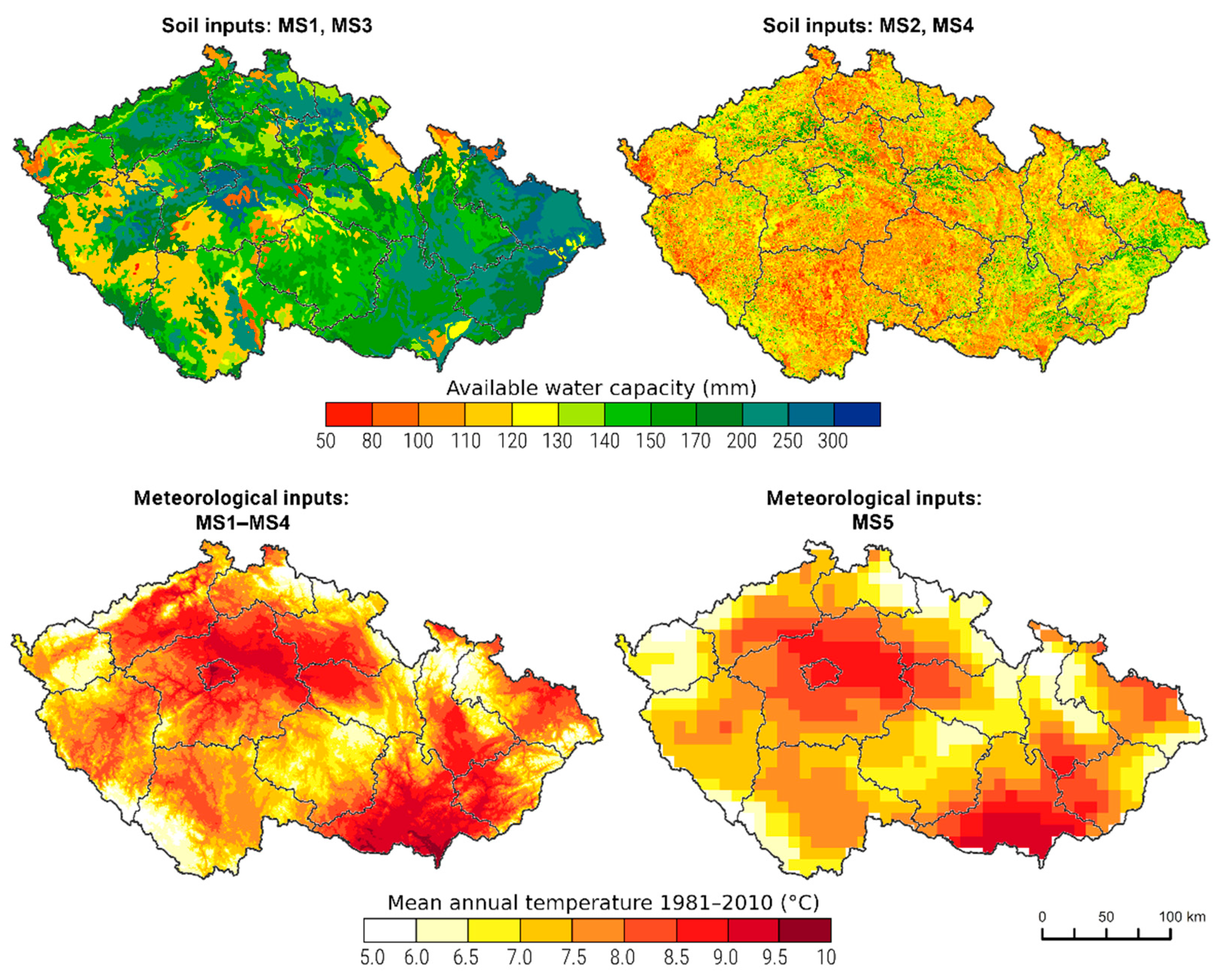
2.1. Study Area

This study was conducted for the territory of the CR, a state located in central Europe. The CR has a total area of 78,866 km2, with altitudes ranging from 115 to 1603 m (mean altitude 390 m asl). In terms of land-use structure, agricultural land cover takes up more than half of the territory (53.3%) with arable land accounting for 37.2%, permanent grasslands for 13.0%, and other agricultural land for 3.1% [14]. More than a third of the CR (33.9%) is covered by commercial forests, followed by built-up area (10.7%). Bodies of water take up 2.1% of the country.

2.2. Soil Moisture Model and Model Setups

The SoilClim water balance model [9] was employed to simulate soil moisture and quantify drought. The volumetric soil moisture was converted to “relative soil saturation” (AWR), in which 100 represents field capacity and 0 stands for wilting point. Five model setups (MS1–MS5) were employed herein for calculation of the soil moisture relevant to operational application of drought monitoring at national to global scales (Figure 1). A detailed overview presenting the differences between the MS setups 1–5 appears in Table A1, Appendix A.
MS1 lay at the core of soil moisture modelling during 2014–2020 within CDMS. The MS1 setup is based on a two-layer (0.0–0.4 m and 0.4–1.0 m) soil-water balance-bucket approach. The soil moisture in these layers is the result of the relationship between inflow and outflow water-balance components. The inflow components consist of infiltration of water from precipitation and snowmelt, while the outflow results from evapotranspiration and deep percolation. The evapotranspiration routines are based on a single-crop coefficient (Kc) approach [15] with modifications described by Hlavinka et al. [9]. At the heart of these modifications is the dynamically changing crop coefficient as a function of growing degree days (GDD). The parameterization of Kc and root depth is based on the Corine land cover map (CLC 2006; version 12/2009) with a grid resolution of 100 × 100 m. Percolation from a soil layer occurs whenever the water content exceeds field capacity, while a partial percolation is also factored for water content below field capacity; the latter allows for the effect of macropores [9]. While percolation from the top layer consists of an inflow of water to the bottom layer, percolation from the bottom layer is considered as water loss from the entire system (i.e., deep percolation). The available water capacity (AWC)—the difference between field capacity and wilting point—was estimated in MS1 through combination of parameters from the soil-type map by Tomášek [16] and detailed physical characteristics of the soil from 1073 pits, collected as part of the Czech National Soil Survey (for more details see [10]). The water-holding capacity was calculated on the assumption of a 1.0-m-deep soil profile unless the database indicated a shallower soil depth. The input meteorological variables included daily minimum and maximum air temperatures (Tmin, Tmax, °C), daily mean vapor pressure (e, kPa), daily sum of global radiation (Rg, MJ m−2), daily mean wind speed (u, m s−1), and daily precipitation total (P, mm) in the form of gridded data at a resolution of 500 × 500 m, all based on Czech Hydrometeorological Institute (CHMI) station observations. Daily climatological observations were subject to thorough quality control and homogenization [17] and were spatially interpolated on the basis of regression kriging using terrain features (e.g., altitude, slope) as predictors.
The MS2 setup was based on a modelling scheme nearly identical to that of MS1. The only difference lay in AWC; in MS2, this was based on a new dataset provided by the Research Institute for Soil and Water Conservation [18], and on topsoil physical properties for Europe from the LUCAS 2015 topsoil dataset [19]. Differences between these two AWC versions appear in Figure 2.
In contrast to MS1 and MS2, setups MS3 and MS4 were based on a different modelling scheme, applying four soil layers in the SoilClim model (0.0–0.1, 0.1–0.4, 0.4–1.0, and 1.0–3.0 m) and also a deeper root system (Table A1). Further, while the inflow components of water balance are identical to those of MS1 and MS2, the outflow components of MS3 and MS4 feature a number of differences. Firstly, the evapotranspiration is based on the dual Kc approach, in which evaporation (from soil and interception) and transpiration are addressed separately. Secondly, percolation is approached in the same way as in MS1 and MS2, but partial percolation is not allowed for in the deepest layer. This rests on the assumption that, soil water content from the lowest layer cannot decrease below field capacity when there is no water uptake by roots. Thirdly, runoff based on a curve number approach [20] is implemented in MS3 and MS4, thus reducing infiltration as a response to precipitation rate, curve number, slope, and antecedent soil moisture in the topsoil. Finally, in contrast to MS1 and MS2, MS3 and MS4 assume dynamically changing root depth in field crops, proportional to the dynamics of Kcb driven by GDD. The input data for MS3 are identical to those for MS1, while the input data for MS4 are identical to those for MS2.
The MS5 setup, used for global drought monitoring, was of an almost identical model structure to that of MS3 and MS4, but Kcb was not a function of GDD, but of leaf area index (LAI), as adopted from ERA5-Land reanalysis data. For MS5, the meteorological data input consisted of the Climate reanalysis ERA5-Land available at a spatial resolution of 0.1° × 0.1° from 1981 until the present. The production of ERA5-Land is based on the tiled ECMWF Scheme for Surface Exchanges over Land incorporating land surface hydrology (H-TESSEL). To monitor its simulated land fields, ERA5-Land inputs ERA5 atmospheric variables (temperature and air humidity), “atmospheric forcing”, while ERA5 features a coarser reanalysis available at a resolution of 0.25° × 0.25°. Thus, while observations are not used directly in the production of ERA5-Land, they exert an indirect influence through atmospheric forcing from ERA5-Land, which assimilates a vast quantity of in-situ and satellite observations. The input air temperature, air humidity, and pressure used to run ERA5-Land were corrected to allow for altitude differences between the grid of the forcing and the higher resolution grid of ERA5-Land, using what is known as “lapse rate correction”. Since ERA5-Land is available in hourly time steps, the data were aggregated into daily values for the SoilClim model. The original inputs from ERA5-Land were precipitation, temperature at 2 m, dew-point temperature at 2 m, wind speed at 10 m, and incoming short-wave radiation. The derived daily values required for the SoilClim model were the same as those for MS1–MS4 and were recomputed into the required variables and units from ERA5-Land. In addition, LAI for high and low vegetation categories from ERA5-Land and the associated high vegetation and low vegetation cover fractions were considered (in contrast to MS1–MS4, in which CLC 2006 was employed) to simulate canopy height, root depth, and transpiration, together with the ERA5-Land orography for the purpose of surface runoff simulation. An example of differences between MS1–MS4 and MS5, in terms of mean annual temperature input, appears in Figure 2.

2.3. Methods

Comparison of drought anomalies between the SoilClim model setups was enabled by converting the AWR data calculated from SoilClim values into percentiles of the 1961–2010 period, created individually for every grid point, date, and soil profile. In order to address actual soil drought, values below the 10th percentile were also involved. The selection of 10th-percentile drought is in conformity with its use in US Drought Monitoring since 1995 [21,22] and in CDMS [2,8], as well as with several publications addressing the same limit (e.g., [12,13]). The gridded data were then aggregated for the entire CR, using the percentage of grid points fulfilling the 10th-percentile drought condition for every day. The aggregated time series were applied in selection of soil-drought episodes from the MS1–MS4 series according to the three following criteria:
(i)
During a drought episode, at least 75% of grid points over the territory of the CR had to report a 10th-percentile drought on at least one day.
(ii)
The onset of the episode occurred when at least 50% of the grid points reported 10th-percentile drought; it ended when the figure dropped below 50%.
(iii)
A decline to below 50% of grid points reporting 10th-percentile drought of up to 5 days was not counted as interruption of the drought episode.
The areal extent and temporal variability of soil droughts in the 1961–2020 period was analyzed in terms of the MS1–MS4 results, with particular emphasis on their differences. MS5, with data reaching back to only 1981, was not included in this part of the study. Long-term variability was characterized by linear trends and similarities between MS1–MS4 characterized by Pearson correlation coefficients and paired t-tests. Their statistical significance was evaluated at a significance level of 0.05. Inter-annual variability in differences among MS1–MS4 was further analyzed in terms of the annual cycle of AWR in the 0–40 cm and 40–100 cm soil layers.
A simpler and more widely-used drought index, the Palmer Drought Severity Index (PDSI), after Palmer [23], was selected for comparisons with the SoilClim model results. In general, PDSI is based on the supply-and-demand concept of the water balance equation and thus incorporates antecedent precipitation, moisture supply, and demand at the surface. The version of self-calibrated PSDI [24] employed was modified to estimate surface demand, using a reference evapotranspiration calculated according to Penman-Monteith method as formulated by Allen et al. [15]. The soil parameters were set on the basis of the same database as that described for MS2 and MS4 [18]. The PDSI series were calculated on 500 × 500 m grids, using the same database as that for the MS1–MS4 calculations. Monthly PDSI values were converted into 10th-percentile values and then compared with soil drought series, calculated for the purposes of simplification from the MS4 setup, which uses the same soil inputs and the more advanced version of the model algorithm (Table A1).
MS4 and MS5 were employed to compare high-resolution and low-resolution setups for the 1981–2020 period. MS4 was selected as the most recent setup, currently used in CDMS, while MS5 was developed as the first lower-resolution version of SoilClim for monitoring global drought. Long-term variability in MS4 and MS5 was characterized by linear trends and Pearson correlation coefficients (significance level 0.05).
In the main, the results of the analysis are presented for non-standard seasons: January–March (JFM), April–June (AMJ), July–September (JAS), and October–December (OND). This choice of non-standard seasons was made to establish continuity with many previous studies conducted for the summer (April–September) and winter (October–March) half-years (e.g., [12,13]), and those that worked directly with those seasons (e.g., [11,25]). Moreover, they correspond closely to the annual AWR cycle in the CR.
The Pearson correlation coefficient was used to characterize degrees of similarity among different soil drought series calculated by the SoilClim model setups. The paired t-test was used to establish the significance of differences in pairs of these series. Linear trends were also calculated, and their significance was evaluated by t-test at a significance level of 0.05. Trends of the soil drought series were also assessed by Mann-Kendall test at a significance level of 0.05.

3. Results

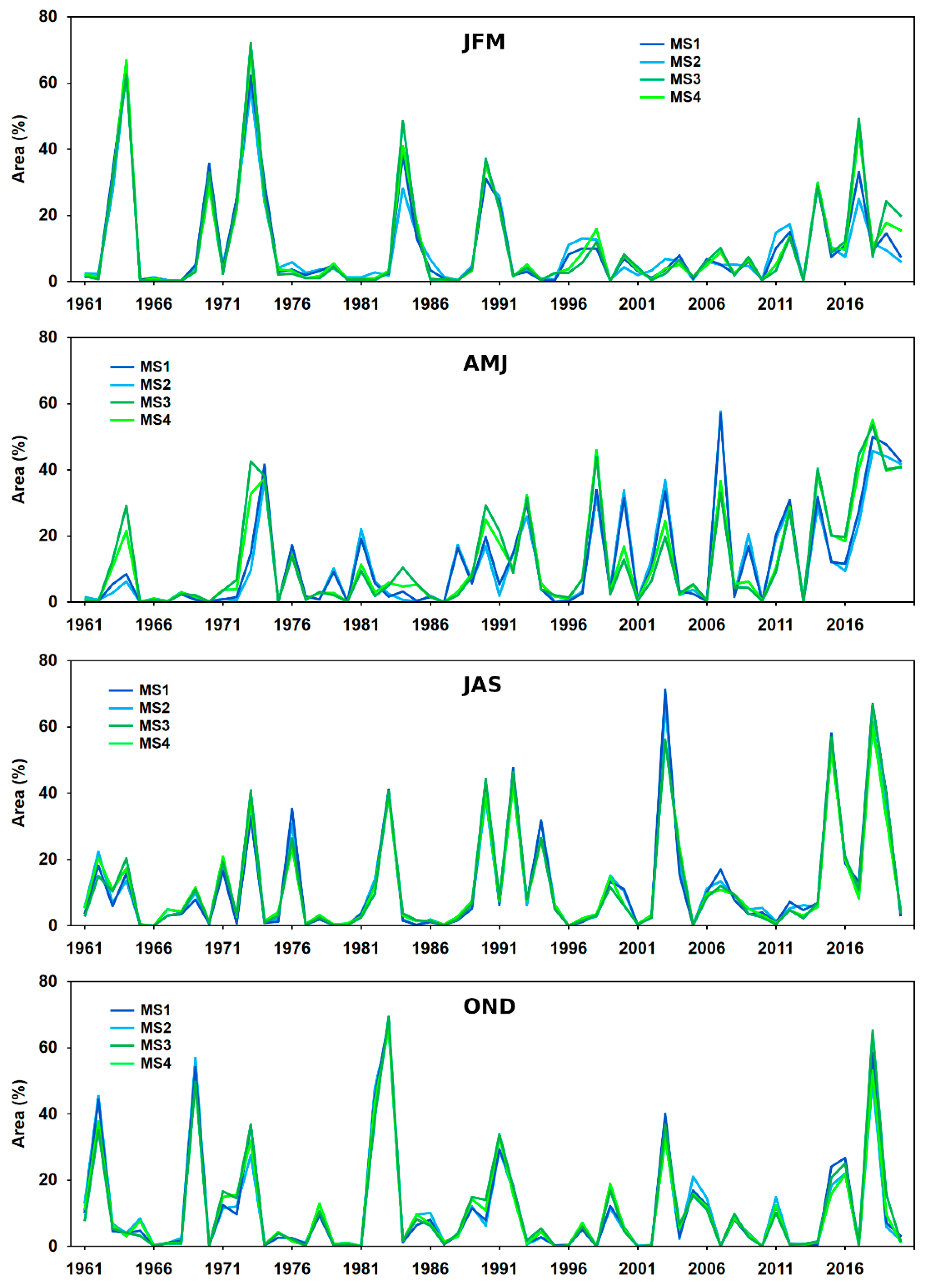
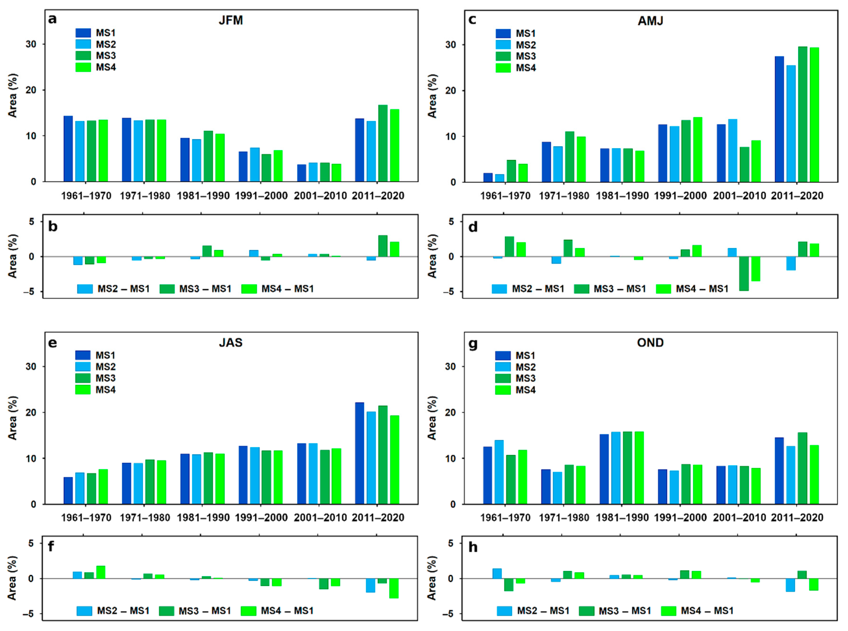
3.1. Areal Extent and Temporal Variability of Soil Drought

The areal extent and temporal variability of soil droughts in the CR according to MS1–MS4 SoilClim model setups, expressed as mean percentages of the grid points with 10th-percentile drought in JFM, AMJ, JAS, and OND in the 1961–2020 period in the 0–100 cm soil layer, appears in Figure 3. Close agreement among the four setups in the occurrence of individual drought episodes, especially in JAS and OND, is apparent, but episodes sometimes differ in terms of severity, largely in JFM and AMJ, in which MS3 and MS4 indicate larger areas of drought in certain cases.
Figure 3 shows that the main drought episodes (exceeding an extent of 40% of the CR territory) in JFM occurred in 1964, 1973, 1984, and 2017. In 2017, MS3 and MS4 suggest considerably larger areas affected than those that appear in MS1 and MS2. In AMJ, a far higher concentration of the main drought episodes occurs in the second half of the 1961–2020 period; the main episodes occurred in 1973–1974, 1998, 2007, 2014, and 2017–2020. In JAS, such episodes occurred in 1983, 1990, 1992, 2003, 2015, and 2018, while in OND they took place in 1962, 1969, 1982–1983, 2003, and 2018.
Fluctuations of areas with 10th-percentile soil drought shown at annual resolution (Figure 3) may be aggregated into decadal values, as demonstrated in Figure 4. The differences among the four setups are at their lowest for JAS and OND, while in JFM and especially AMJ, there are well-expressed differences between the MS1–MS2 and MS3–MS4 pairs and some other differences beyond this division. The last decade, 2011–2020, is characterized by the highest extent of soil drought (particularly for AMJ and JAS), except in OND.
Correlation analysis of the soil drought series yields statistically significant Pearson correlation coefficients, exceeding 0.90, among all four model setups for all seasons investigated. Pairs consisting of one MS1–MS2 setup and one MS3–MS4 setup have slightly lower correlation coefficients, sometimes below 0.95 for JMF and AMJ. On the other hand, MS1–MS2 and MS3–MS4 pairs exhibit coefficients of up to 0.99. Application of the paired t-test to pairs of soil drought series yields no statistically significant differences.
Linear trends in areas exhibiting 10th-percentile soil drought (Table 1) are all slightly negative and statistically non-significant in JFM, lower for MS1 and MS2 than for MS3 and MS4. In AMJ, all trends are positive and statistically significant, with values exceeding 4.0%/10 years in MS1 and MS2 or around 3.5%/10 years in MS3 and MS4. All trends are positive in JAS, but only that of MS1 is statistically significant. All trends are statistically non-significant in OND, with values ranging from –0.61 to 0.21%/10 years. The significance of the Mann-Kendall test is consistent with the significance of linear trends in all cases.

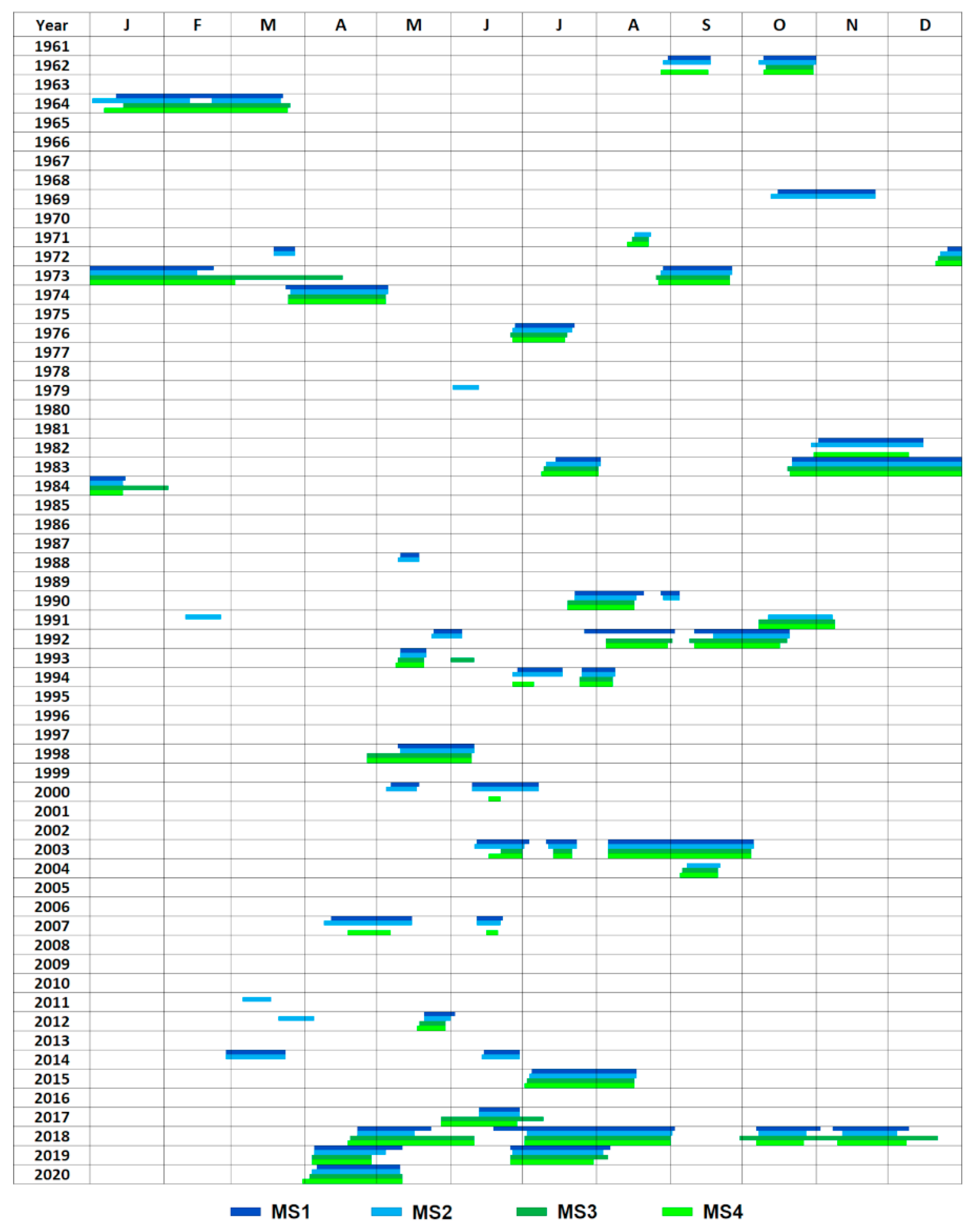
3.2. Episodes of Soil Drought

The temporal variability of 10th-percentile soil drought episodes within individual years in the 1961–2020 period appears in Figure 5, categorized by the first four SoilClim model setups. In JFM and OND, drought episodes generally occurred more often before 1990, and were longer and less frequent than in April–September. On the other hand, in JAS, and particularly in AMJ, drought episodes were much more frequent after 1990, with a marked concentration at the end of the period analyzed. This corresponds with the trends presented in Section 3.1, although it appears even more distinct here. The four SoilClim model setups agree largely upon the existence of individual drought episodes, although their beginnings and ends often differ. In addition, some episodes, particularly in JFM and AMJ, appear in only some of the model setups (e.g., in April–May 2007 and March 2014).
Table 2 presents detailed information on the numbers of days within soil drought episodes and their percentage agreement for individual model setups. JFM returns the lowest number of days of soil drought episodes, ranging from 160 to 207. Further, there is a high degree of disparity in percentage agreement among individual pairs of setups, which varies from 58.9 to 94.4%. In AMJ, there are between 295 and 365 days within drought episodes, with slightly higher numbers for MS1 and MS2. The variation range of percentage agreement is also very high (45.6–82.3%) and the MS1–MS2 and MS3–MS4 pairs show significantly higher percentage agreement (73.7–82.3%) than the other pairs (45.6–67.2%). JAS contains the highest number of days within drought episodes, ranging from 403 to 438 days (and also the highest percentage agreement, ranging from 81.1 to 94.5%). This is followed by the percentage agreement in OND, which ranges from 66.6 to 94.0%; however, the numbers of days are far lower (240–290).

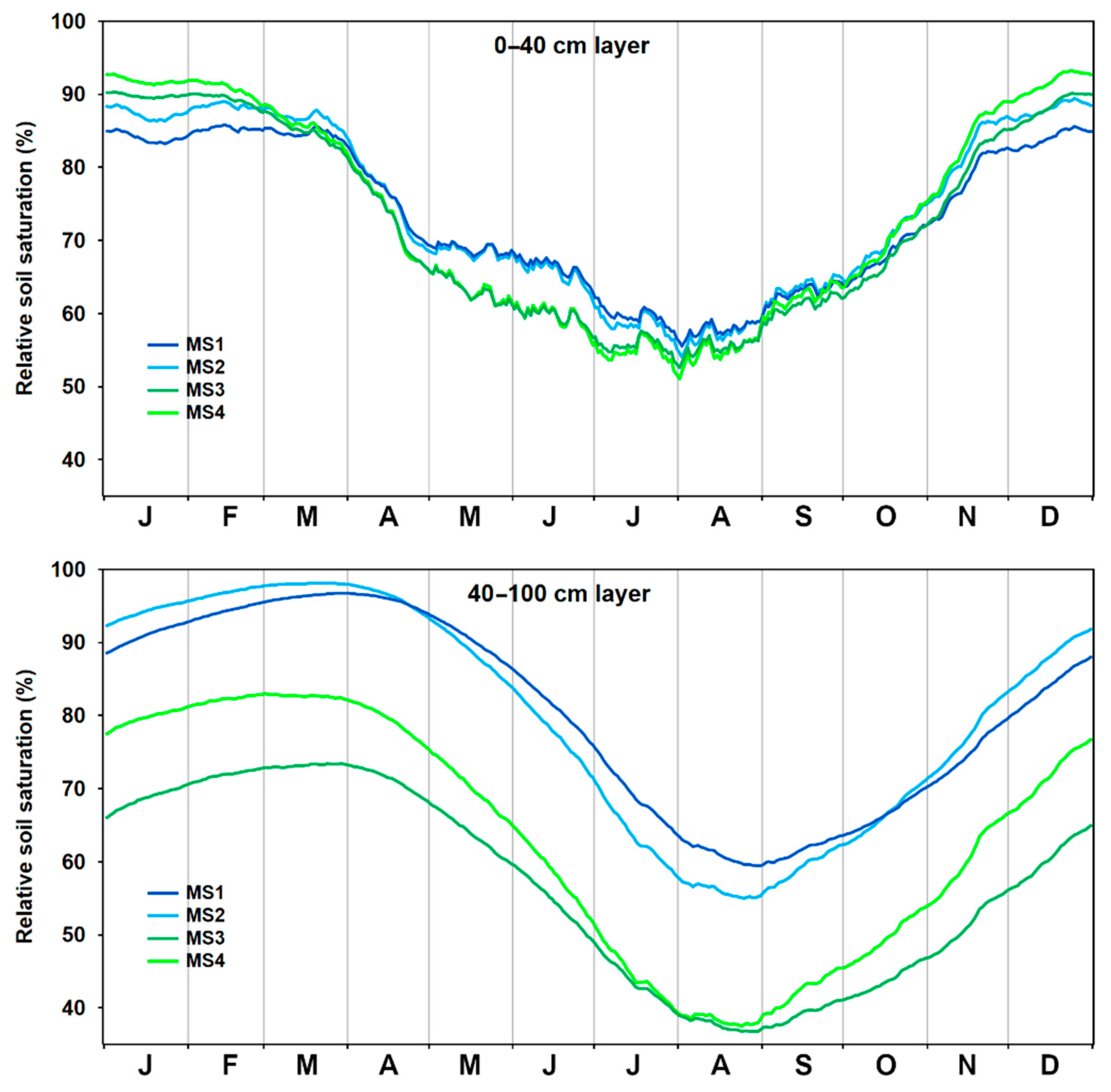
3.3. Relative Soil Saturation

In order to investigate the differences disclosed between the four SoilClim model setups, particularly between MS1–MS2 and MS3–MS4 pairs, the mean annual variations of AWR in the 0–40 cm and 40–100 cm layers were examined (Figure 6). In the upper layer, 0–40 cm, AWR remains stable at around 85–90% in January–March with the highest values for MS4 and lowest for MS1. A rapid decrease within all model setups follows in April, most marked for MS3 and MS4. Their values stay 5–10% below MS1 and MS2 in May–July, while values for all four setups decrease slowly, then almost close the gap in July. A mean annual minimum of 55–60% is reached in early August within all four model setups. Their values are nearly identical in August–October, steadily increasing. The values of individual setups begin to differ in November–December, but they all indicate an increase until the annual maximum in late December.
MS3 and MS4 values for the 40–100-cm layer are approximately 10–20% lower compared to MS1 and MS2 throughout the whole year. There is also a difference in annual amplitude, which is lower in MS1 and MS3, higher in MS2 and at its highest in MS4. However, the shape of the curve of annual variation is very similar for all model setups, with a maximum in March and a minimum in late August.

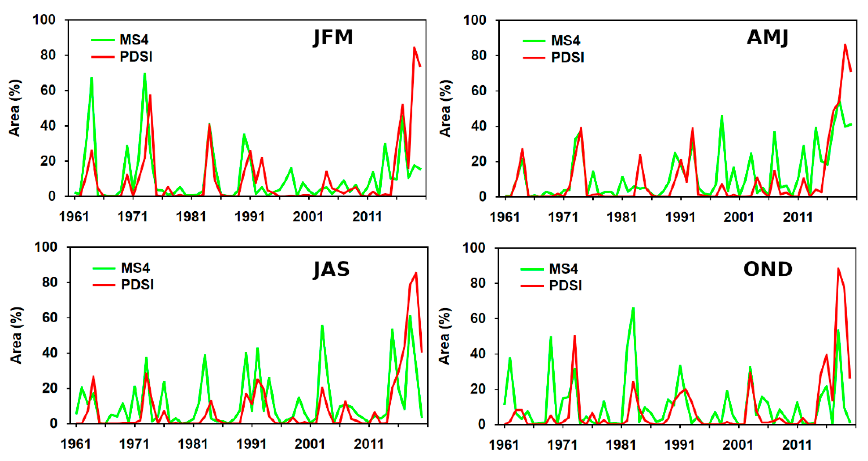
3.4. Model Setups and PDSI

The MS4 results indicate more years with marked drought occurrence (Figure 7). PDSI agrees with MS4 for some years, but does not show increased drought occurrence in others disclosed by MS4. On the other hand, drought is indicated in only very few years by PDSI alone. For multi-year drought, PDSI sometimes appears to indicate drought onset, but with a delay compared to MS4; however, steady drought accumulation follows. This trend is most distinctive in 2018 and 2019, when a five-year drought episode culminated. PDSI indicates an extremely large area with 10th-percentile drought (close to 100%), while for MS4 is the corresponding area smaller.
Seasonal and half-year linear trends of MS4 and PDSI appear in Table 3. They exhibit statistically significant positive trends in AMJ and the summer half-year (SHY), and only for PDSI values in JAS and OND. Non-significant trends in both variables appear in JFM and the winter half-year (WHY), although with different trends. Absolute values of trends calculated for MS4 are always lower than those for PDSI, except in AMJ. The Mann-Kendall test does not indicate a significant trend for PDSI in OND, but it is consistent with the significance of linear trends in all other cases.

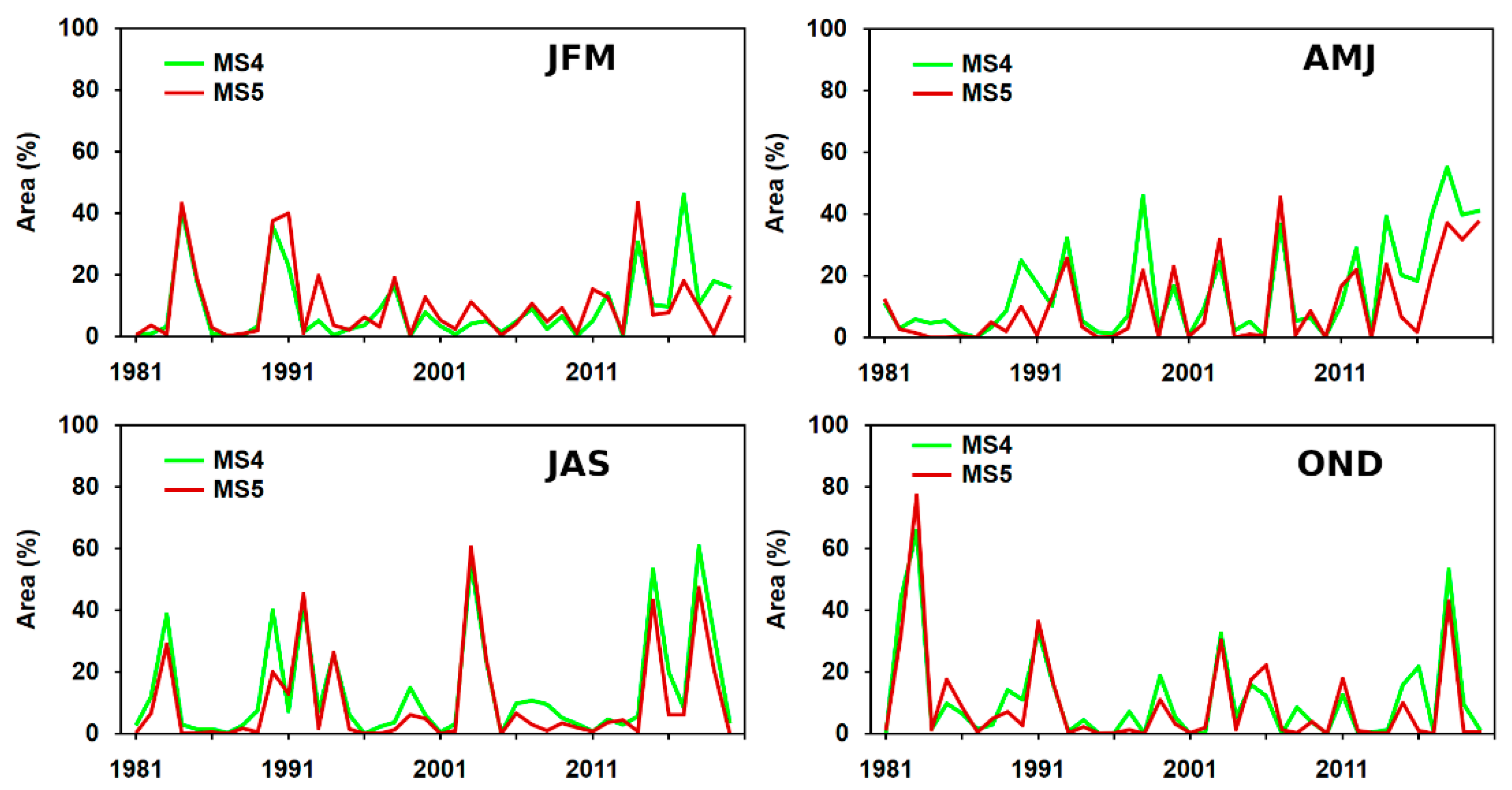
3.5. Soil Drought in MS4 and MS5

The variability of soil drought in the CR according to MS4 and MS5, expressed as mean percentages of grid points with 10th-percentile drought in JFM, AMJ, JAS, and OND in the 0–100-cm soil layer for the 1981–2020 period, appears in Figure 8. Stronger agreement between the two setups occurs in JAS and OND. The differences for seasons appear to be randomly distributed. In terms of JFM, considerable differences occurred in 2017 and 2019. For AMJ, large differences appeared in 2014–2019 and further in 1990 and 1998. This shows that differences are particularly marked towards the end of the period analyzed.
Correlation coefficients demonstrate that there are much larger differences between MS4 and MS5 in JFM and AMJ than among MS1–MS4 pairs; their values achieve only 0.81 and 0.86 compared with coefficients over 0.90 in all MS1–MS4 pairs (Table 4). The positive linear trends for the 1981–2020 period show higher values for MS4 than for MS5, but they are statistically significant only in AMJ and SHY for both MS4 and MS5 setups. The Mann-Kendall test indicates a significant trend for MS4 also in JFM, but it is consistent with the significance of linear trends in all other cases. The MS5 setup indicates deeper decreases in OND and WHY than MS4, but these trends are statistically non-significant.

4. Discussion

4.1. Model Uncertainties

As pointed out in Section 2.2, the definitions of drought characteristics herein were derived from five setups of the SoilClim model. MS1–MS4 employed daily weather data collected by the CHMI in a station network of almost 800 rain-gauge stations and some 250 climatological stations. The mean distance between neighboring stations is c. 22–30 km for climatological stations and c. 10 km for rain-gauge stations. A locally-weighted regional regression, taking elevation and other terrain characteristics into account, was employed to interpolate the daily data into 500 × 500 m grids. Although the daily global radiation balance considered slope, aspect and horizon obstruction [26], uncertainties associated with the nature of the ground data cannot be ignored.
In addition to a certain lack of precision in the input data, other uncertainties are intrinsic to the model itself. For example, the module for actual evapotranspiration and soil-water content in the SoilClim model simplifies otherwise complex, three-dimensional soil-water transport processes by using only two (MS1–MS2) or four (MS3–MS5) soil layers and the “bucket approach”. SoilClim estimates of soil-moisture content are substantially affected by the estimated maximum soil-water holding capacity for the soil layers in each grid, while considerable variation also exists at the sub-grid scale. Because the SoilClim model setups use three different soil inputs (described in Section 2.2), the maximum soil-water holding capacity for individual grids may differ dramatically.
Within grids where the soil water balance is, at least for some part of the growing season, influenced by the presence of a shallow water table, the relative water content in the lower soil layers cannot fall below a specific threshold. This strategy is applied to allow for the fact that soils with an observed gleyic process in close proximity to major water bodies, peat, and bog areas have significantly slower soil-moisture depletion rates than neighboring grids lacking these influences [11]. Such simplifications, and many others, arise naturally out of large-scale modelling schemes and data availability. However, to assess the intensity and duration of drought episodes, the soil moisture anomaly (a percentile-based value) has been used herein, thus eliminating the effect of uncertainties in specific soil-water processes and describing droughts as climatological phenomena in a process-based manner.

4.2. Different Models Setups and Expression of Soil-Drought Episodes

In the first half of the year, few important differences were disclosed in the analyses for MS1–MS4 during the 1961–2020 period. The MS1–MS2 and MS3–MS4 pairs yielded more similarities in both soil-drought extent and occurrence or soil-drought episodes than was the case in comparison across these pairs. Most of the differences are also much higher in JFM and AMJ than in JAS and OND when the differences are often marginal. This indicates that changes in the model algorithm, conducted evenly for MS3 and MS4 compared to MS1 and MS2 (see Table A1) have stronger impacts on the results than different soil inputs, which are the same for MS1/MS3 and MS2/MS4 pairs, despite large differences in soil-water holding capacity between the soil inputs (Section 2.2).
The larger differences in JFM and AMJ appear to arise out of a more rapid decrease in AWR in the 0–40-cm soil layer in MS3 and MS4 compared to MS1 and MS2 (Figure 5). There could be a number of reasons for this phenomenon. The MS3 and MS4 setups use more advanced ways of computing the evapotranspiration dual-crop coefficient approach (Section 2.2), which takes non-constant the bare-soil to reference evapotranspiration ratio into account, affecting the actual evapotranspiration calculated, largely in winter and early spring (i.e., before or after the soil is covered by vegetation). Because the soil moisture is, on average higher during these two seasons, MS3 and MS4 exhibit higher actual evapotranspiration than MS1 and MS2 in this part of the year.
A further reason for the differences may be the use of the dynamic depth of the roots in MS3 and MS4, while MS1 and MS2 keep this value constant. Thus in spring, when vegetation starts to consume more soil water, this is obtained largely from the upper soil layer, before the simulated roots grow deeper, which also corresponds with a more rapid decrease in AWR in the 0–40-cm soil layer. Other possible influences might include different calculations of water runoff from rain and melted snow cover, or varying criteria for constant infiltration of water from the upper to the lower soil layers (Section 2.2).
These differences also lead to a larger gap in AWR for MS3 and MS4 compared to MS1 and MS2 in the 40–100 cm layer, while the course of annual variation is almost the same for all setups. But because the percentile-based soil-drought used in the study is not primarily affected by the mean level of AWR, but by its variation, the differences in the 0–40 cm layer are more crucial, despite mean annual values differing marginally.
The MS5 setup (analyzed only for the 1981–2020 period) uses a model algorithm very similar to that of MS3 and MS4, but its meteorological, land-use, and terrain inputs are derived from ERA5-Land reanalysis, with the grid simplified to corresponding resolution and soil inputs using SoilGrids [27,28]. This led to larger differences than those disclosed among MS1–MS4, even when compared to the MS4 algorithm, the most similar, alone. Most of the differences appear to be concentrated around the final dry period in 2014–2019, when MS5 indicates a smaller area affected by 10th-percentile drought. In consequence, lower values are generated for the linear trend over the 1981–2020 period in all seasons when compared to MS4. In order to investigate the drivers of the differences, the meteorological inputs for MS4 and MS5 were compared (Table 5). Although no significant linear trends were found for variables in the series of seasonal differences, the mean values of the differences differ substantially. MS5 inputs (ERA5-Land reanalysis) for the mean temperature are lower by c. 1.6 °C for AMJ and JAS and by c. 0.5 °C for JFM and OND compared with MS4 inputs (CHMI data). In addition, MS5 inputs indicate a higher precipitation total, by 28–37 mm on average for all seasons (133 mm annually). This is only partially compensated for by the reference evapotranspiration being higher for MS5 inputs by c. 20 and 24 mm in AMJ and JAS and by only c. 4 and 6 mm in JFM and OND (54 mm annually).
Although these differences are evident throughout the entire 1981–2020 period, they were probably of the highest impact during the extended 2014–2019 soil-drought episode. Such conditions dictated that soil moisture values were very often close to the threshold of 10th-percentile drought. In the case of the colder and wetter MS5 data, the resulting values did not cross the drought threshold in such a substantial proportion of cases as that calculated using MS4 data.
In the PDSI time series, the area of the 10th-percentile drought in the 2014–2019 episode is markedly larger for all seasons when compared with MS4 results and the remainder of the 1961–2020 period. This may also be one of the reasons why linear trends in PDSI are higher than those in MS4 for all seasons, except AMJ (Table 3). The method of PDSI calculation is responsible for this. PDSI employs accumulation of water-balance anomalies (Z-index) over a longer period [23] and therefore short-term wetter periods during long drought episodes do not influence PDSI values significantly. In contrast, in the MS4 setup, the SoilClim model calculates AWC in daily steps and reveals even short-term increases in AWC, leading to temporary decreases in the area affected by soil drought; it also decreases seasonal means of the affected area during long-term drought episodes. The largest difference in linear trends between PDSI and MS4, for OND (Table 3), is probably caused by extended PDSI accumulation during dry summer half-years in the 2014–2019 drought episode contrasting with rapid AWC increases during wetter OND in MS4. The previous drought episodes were rather isolated, while in the 2014–2019 period (especially in 2018 and 2019), there were several drought episodes in sequence (Figure 5), separated only by a few weeks or months. This led to the described accumulation of the PDSI index values, which subsequently indicated extremely large mean area affected by drought in those years (according to the PDSI), which did not occur in previous cases.
Soil-moisture and soil-drought frequency trends in the CR have been investigated by several previous studies (e.g., [11,12,13]), covering various regions within the CR and neighboring areas. Statistically significant positive trends in soil drought frequency emerged in most cases for the summer half-year (October–March) and non-significant, almost zero or negative trends, for the winter half-year (April–September). These accord with the findings of this study, which incorporates the whole area of the CR, although the summer half-year was further divided herein into AMJ and JAS seasons and higher trends were found for AMJ, while values for trends in JAS were roughly halved and were not statistically significant in three of the MS1–MS4 setups. This is probably related to a statistically significant decrease in AMJ precipitation compared to the increasing trend in JAS totals in the CR during 1961–2019, as shown by Brázdil et al. [29].
AMJ had already been indicated as the season with the most significant increase in drought frequency and/or decline in soil moisture by Trnka et al. [11]. However, the data used for the Trnka study covered only the period up to 2012 and only one SoilClim model setup (similar to MS1) was employed. They identified temperature and precipitation as the most important factors influencing, among other things, the values for soil-moisture/drought. While precipitation is the only source of water for the soil, temperatures contribute directly to its reduction through evaporation; prolongation of the vegetation season also contributes to higher transpiration and a shorter freezing period leads to a reduction in the period of snow accumulation. In terms of linear trends, the mean annual temperature in the CR exhibited a strong positive and statistically significant trend (0.36 °C/10 years) in the 1961–2020 period, but a non-significant linear trend in annual precipitation stood close to zero (−0.3 mm/10 years) (see also [29,30]).

5. Conclusions

From the analysis of 10th-percentile soil drought over the territory of the CR during the 1961–2020 period based on five model setups, the following conclusions may be drawn:
(i) According to all SoilClim model setups (MS1–MS5), there is a strong, statistically significant increase in the occurrence of 10th-percentile soil drought in AMJ. The increase in JAS is statistically significant only for MS1, while OND and JFM exhibit statistically non-significant trends.
(ii) MS1–MS2 and MS3–MS4 exhibit notable differences only for JFM and AMJ, a result of more rapid mean AWR decrease in the 0–40-cm soil layer in MS3–MS4. This arises largely out of more advanced approaches to estimation of evapotranspiration, calculation of runoff and internal percolation, and consideration of the dynamic depth of roots in the improved algorithm used in MS3–MS4. Different soil input data had less effect than different modelling schemes.
(iii) Percentage agreement in the 10th-percentile soil drought episodes varied among MS1–MS4 setups and individual seasons, providing similar patterns to those of the differences in soil drought frequency. The majority of the delimited episodes appeared in all model setups.
(iv) The SoilClim model is able to depict the variability of soil drought occurrence in greater detail than the widely-used PDSI, which tends to capture only the most severe events.
(v) Deployment of the MS5 setup, developed with its major simplification of the model grid for the use in global-scale drought modeling, still leads to an acceptable conformity of results with MS4 with finer resolution. Some of the non-conformities may be explained by substantial differences between meteorological inputs from the ERA5-Land dataset and from gridded CHMI station data.
(vi) The MS4 setup can be considered as the best scenario of five versions of SoilClim model for soil-drought modelling, particularly due to more accurate representation of soil processes. Although, high consistency with setups MS1–MS3 does not change results of soil-drought analyses significantly.

Author Contributions

Conceptualization, R.B., M.T.; methodology, J.Ř., R.B., M.T., M.F.; formal analysis, J.Ř., R.B.; data curation, J.B., P.Š., P.Z.; writing, review, and editing, J.Ř., R.B., M.T., M.F.; visualization, J.Ř., D.S., M.B. All authors have read and agreed to the published version of the manuscript.

Funding

This research was funded by the Ministry of Education, Youth and Sports of the Czech Republic for SustES—Adaptation strategies for sustainable ecosystem services and food security under adverse environmental conditions project ref. CZ.02.1.01/0.0/0.0/16_019/0000797. J.Ř. also received funding from Masaryk University within the MUNI/A/1570/2020.

Acknowledgments

We would like to thank Tony Long (Carsphairn, Scotland), who helped work up the English.

Conflicts of Interest

The authors declare no conflict of interest.

Appendix A

Table A1. Basic features of the model setups MS1–MS5 employed for the calculation of the soil moisture. Abbreviations: AWR—relative soil saturation; CHMI—Czech Hydrometeorological Institute; GCRI—Global Change Research Institute; GDD—growing degree days; Kcb—Basal crop coefficient; Ke—soil evaporation coefficient; LAI—Leaf area index.
MS1MS2MS3MS4MS5
Simulation Period
1961–20201961–20201961–20201961–20201981–2020
Meteorological Inputs
CHMI/GCRICHMI/GCRICHMI/GCRICHMI/GCRIERA5-Land [31]
Soil inputs
Soil type map after Tomášek [16]Research Institute for Soil and Water Conservation [18]Soil type map after Tomášek [16]Research Institute for Soil and Water Conservation [18]SoilGrids [27,28]
Land use
CORINE Land Cover 2012 v17CORINE Land Cover 2012 v17CORINE Land Cover 2012 v17CORINE Land Cover 2012 v17ERA5-Land: high and low vegetation, bare ground
Terrain
Digital Elevation Model over Europe (EU-DEM-3035)Digital Elevation Model over Europe (EU-DEM-3035)Digital Elevation Model over Europe (EU-DEM-3035)Digital Elevation Model over Europe (EU-DEM-3035)ERA5-Land
Leaf area index (LAI)
----ERA5-Land
Model scheme
All the MSs feature:
reference evapotranspiration after Allen et al. [15]
snow submodule after Trnka et al. [32]
The MSs differ in:
vegetation submodule
single-crop coefficient changing dynamically as a function of GDDsingle-crop coefficient changing dynamically as a function of GDDdual-crop coefficient where Ke is dependent on topsoil water balance and Kcb changes dynamically as a function of GDDdual-crop coefficient where Ke is dependent on topsoil water balance and Kcb changes dynamically as a function of GDDdual-crop coefficient where Ke is dependent on topsoil water balance and Kcb changes dynamically as a function of LAI
canopy height growing dynamically as a function of GDDcanopy height growing dynamically as a function of GDDcanopy height growing dynamically as a function of GDD up to a crop-specific maximumcanopy height growing dynamically as a function of GDD up to a crop-specific maximumcanopy height growing dynamically as a function of LAI
constant root depth
(1 m)
constant root depth
(1 m)
root depth growing dynamically as a function of GDD up to a crop- specific maximum or 1.6 m root depth growing dynamically as a function of GDD up to a crop-specific maximum or 1.6 mroot depth growing dynamically as a function of LAI up to a maximum of 2 m
runoff submodule
fraction of precipitation (15% for >2 mm precipitation)fraction of precipitation (15% for >2 mm precipitation)curve number approachcurve number approachcurve number approach
interception submodule
canopy precipitation interception consideredcanopy precipitation interception consideredcanopy precipitation interception considered as part of evaporation within dual-crop coefficient approachcanopy precipitation interception considered as part of evaporation within dual-crop coefficient approachcanopy precipitation interception considered as part of evaporation within dual-crop coefficient approach
soil compartments, vertical stratification
0.0–0.4 and 0.4–1.0 m0.0–0.4 and 0.4–1.0 m0–0.1, 0.1–0.4, 0.4–1.0 and 1.0–3.0 m0.0–0.1, 0.1–0.4, 0.4–1.0 and 1.0–3.0 m0.0–0.1, 0.1–0.4, 0.4–1.0 and 1.0–2.0 m
internal drainage and macropore water flow
only if AWR > 0.5only if AWR > 0.5only if AWR > 0.5 and AWR of the layer i-1 < AWR of the layer ionly if AWR > 0.5 and AWR of the layer i-1 < AWR of the layer ionly if AWR > 0.5 and AWR of the layer i-1 < AWR of the layer i

References

  1. Brocca, L.; Ciabatta, L.; Massari, C.; Camici, S.; Tarpanelli, A. Soil Moisture for Hydrological Applications: Open Questions and New Opportunities. Water 2017, 9, 140. [Google Scholar] [CrossRef]
  2. Trnka, M.; Hlavinka, P.; Možný, M.; Semerádová, D.; Štěpánek, P.; Balek, J.; Bartošová, L.; Zahradníček, P.; Bláhová, M.; Skalák, P.; et al. Czech Drought Monitor System for monitoring and forecasting agricultural drought and drought impacts. Int. J. Clim. 2020, 40, 5941–5958. [Google Scholar] [CrossRef]
  3. Zink, M.; Samaniego, L.; Kumar, R.; Thober, S.; Mai, J.; Schäfer, D.; Marx, A. The German drought monitor. Environ. Res. Lett. 2016, 11, 074002. [Google Scholar] [CrossRef]
  4. Pozzi, W.; Sheffield, J.; Stefanski, R.; Cripe, D.; Pulwarty, R.; Vogt, J.; Heim, R.R.; Brewer, M.J.; Svoboda, M.; Westerhoff, R.; et al. Toward Global Drought Early Warning Capability: Expanding International Cooperation for the Development of a Framework for Monitoring and Forecasting. Bull. Am. Meteorol. Soc. 2013, 94, 776–785. [Google Scholar] [CrossRef]
  5. Hao, Z.; AghaKouchak, A.; Nakhjiri, N.; Farahmand, A. Global integrated drought monitoring and prediction system. Sci. Data 2014, 1, 1–10. [Google Scholar] [CrossRef] [PubMed]
  6. Vicente-Serrano, S.M.; Beguería, S.; Lorenzo-Lacruz, J.; Camarero, J.J.; Lopez-Moreno, I.; Azorin-Molina, C.; Revuelto, J.; Morán-Tejeda, E.; Sanchez-Lorenzo, A. Performance of Drought Indices for Ecological, Agricultural, and Hydrological Applications. Earth Interact. 2012, 16, 1–27. [Google Scholar] [CrossRef] [Green Version]
  7. Ochsner, T.; Cosh, M.; Cuenca, R.H.; Dorigo, W.; Draper, C.; Hagimoto, Y.; Kerr, Y.H.; Larson, K.; Njoku, E.G.; Small, E.; et al. State of the Art in Large-Scale Soil Moisture Monitoring. Soil Sci. Soc. Am. J. 2013, 77, 1888–1919. [Google Scholar] [CrossRef] [Green Version]
  8. Interdrought. Available online: www.interdrought.cz (accessed on 24 May 2021).
  9. Hlavinka, P.; Trnka, M.; Balek, J.; Semerádová, D.; Hayes, M.; Svoboda, M.; Eitzinger, J.; Možný, M.; Fischer, M.; Hunt, E.; et al. Development and evaluation of the SoilClim model for water balance and soil climate estimates. Agric. Water Manag. 2011, 98, 1249–1261. [Google Scholar] [CrossRef]
  10. Trnka, M.; Brázdil, R.; Možný, M.; Štěpánek, P.; Dobrovolný, P.; Zahradníček, P.; Balek, J.; Semerádová, D.; Dubrovský, M.; Hlavinka, P.; et al. Soil moisture trends in the Czech Republic between 1961 and 2012. Int. J. Clim. 2015, 35, 3733–3747. [Google Scholar] [CrossRef]
  11. Trnka, M.; Brázdil, R.; Balek, J.; Semerádová, D.; Hlavinka, P.; Možný, M.; Štěpánek, P.; Dobrovolný, P.; Zahradníček, P.; Dubrovský, M.; et al. Drivers of soil drying in the Czech Republic between 1961 and 2012. Int. J. Clim. 2015, 35, 2664–2675. [Google Scholar] [CrossRef]
  12. Řehoř, J.; Brázdil, R.; Trnka, M.; Řezníčková, L.; Balek, J.; Možný, M. Regional effects of synoptic situations on soil drought in the Czech Republic. Theor. Appl. Clim. 2020, 141, 1383–1400. [Google Scholar] [CrossRef]
  13. Řehoř, J.; Brázdil, R.; Trnka, M.; Lhotka, O.; Balek, J.; Možný, M.; Štěpánek, P.; Zahradníček, P.; Mikulová, K.; Turňa, M. Soil drought and circulation types in a longitudinal transect over central Europe. Int. J. Clim. 2021, 41, 2834–2850. [Google Scholar] [CrossRef]
  14. Czech Statistical Office. Available online: www.czso.cz (accessed on 11 July 2021).
  15. Allen, R.G.; Pereira, L.S.; Raes, D.; Smith, M. Crop Evapotranspiration (Guidelines for Computing Crop Water Requirements); FAO Irrigation and Drainage Paper No. 56; Food and Agriculture Organization of the United Nations (FAO): Rome, Italy, 1998. [Google Scholar]
  16. Tomášek, M. Půdy České republiky (Soils of the Czech Republic); Czech Geological Service: Prague, Czech Republic, 2007. [Google Scholar]
  17. Štěpánek, P.; Zahradníček, P.; Farda, A. Experiences with data quality control and homogenization of daily records of various meteorological elements in the Czech Republic in the period 1961–2010. Időjárás 2013, 117, 123–141. [Google Scholar]
  18. Vopravil, J.; Khel, T.; Heřmanovská, D.; Holubík, O.; Huislová, P. The Map Definition of Water Retention Capacity Characteristics in Agricultural and Non-Agricultural Soils with Territorial Categorization within the Czech Republic; Certificate No. 8/14130-MZe-2018; Research Institute for Soil and Water Conservation: Prague, Czech Republic, 2018. [Google Scholar]
  19. Ballabio, C.; Panagos, P.; Monatanarella, L. Mapping topsoil physical properties at European scale using the LUCAS database. Geoderma 2016, 261, 110–123. [Google Scholar] [CrossRef]
  20. Rosa, R.D.; Paredes, P.; Rodrigues, G.C.; Alves, I.; Fernando, R.M.; Pereira, L.S.; Allen, R.G. Implementing the dual crop coefficient approach in interactive software. 1. Background and computational strategy. Agric. Water Manag. 2012, 103, 8–24. [Google Scholar] [CrossRef]
  21. U.S. Drought Monitor. Available online: http://droughtmonitor.unl.edu/ (accessed on 24 May 2021).
  22. Svoboda, M.; LeComte, D.; Hayes, M.; Heim, R.; Gleason, K.; Angel, J.; Rippey, B.; Tinker, R.; Palecki, M.; Stooksbury, D.; et al. The Drought Monitor. Bull. Am. Meteorol. Soc. 2002, 83, 1181–1190. [Google Scholar] [CrossRef] [Green Version]
  23. Palmer, W.C. Meteorological Drought; Weather Bureau Research Paper No. 45; U.S. Department of Commerce: Washington, DC, USA, 1965. [Google Scholar]
  24. Wells, N.; Goddard, S.; Hayes, M. A self-calibrating Palmer Drought Severity Index. J. Clim. 2004, 17, 2335–2351. [Google Scholar] [CrossRef]
  25. Trnka, M.; Kyselý, J.; Dubrovský, M.; Možný, M. Changes in Central-European soil-moisture availability and circulation patterns in 1881–2005. Int. J. Clim. 2009, 29, 655–672. [Google Scholar] [CrossRef]
  26. Schaumberger, A. Ertragsanalyse im Österreichischen Grünland Mittels GIS unter Besonderer Berücksichtigung Klimatischer Verän-derungen; Diplomarbeit. Technische Universität: Graz, Austria, 2005. [Google Scholar]
  27. Hengl, T.; De Jesus, J.M.; MacMillan, R.A.; Batjes, N.H.; Heuvelink, G.B.M.; Ribeiro, E.; Samuel-Rosa, A.; Kempen, B.; Leenaars, J.G.; Walsh, M.G.; et al. SoilGrids1km—Global Soil Information Based on Automated Mapping. PLoS ONE 2014, 9, e105992. [Google Scholar] [CrossRef] [Green Version]
  28. Hengl, T.; De Jesus, J.M.; Heuvelink, G.B.M.; Gonzalez, M.R.; Kilibarda, M.; Blagotić, A.; Shangguan, W.; Wright, M.; Geng, X.; Bauer-Marschallinger, B.; et al. SoilGrids250m: Global gridded soil information based on machine learning. PLoS ONE 2017, 12, e0169748. [Google Scholar] [CrossRef] [Green Version]
  29. Brázdil, R.; Zahradníček, P.; Dobrovolný, P.; Štěpánek, P.; Trnka, M. Observed changes in precipitation during recent warming: The Czech Republic, 1961–2019. Int. J. Clim. 2021, 41, 3881–3902. [Google Scholar] [CrossRef]
  30. Zahradníček, P.; Brázdil, R.; Štěpánek, P.; Trnka, M. Reflections of global warming in trends of temperature characteristics in the Czech Republic, 1961–2019. Int. J. Clim. 2021, 41, 1211–1229. [Google Scholar] [CrossRef]
  31. ERA5-Land Hourly Data from 1981 to Present. Available online: https://cds.climate.copernicus.eu/cdsapp#!/dataset/reanalysis-era5-land (accessed on 24 May 2021).
  32. Trnka, M.; Kocmánková, E.; Balek, J.; Eitzinger, J.; Ruget, F.; Formayer, H.; Hlavinka, P.; Schaumberger, A.; Horáková, V.; Možný, M. Simple snow cover model for agrometeorological applications. Agric. For. Meteorol. 2010, 150, 1115–1127. [Google Scholar] [CrossRef]
Figure 1. Basic scheme of the SoilClim model depicting the main model submodules. A detailed summary of the differences between the individual model setups appears in Table A1.
Atmosphere 12 00913 g001
Figure 2. Available water capacity in terms of soil inputs for MS1/MS3 [16] and MS2/MS4 [18] setups, and mean annual air temperature in the Czech Republic according to meteorological inputs for MS1–MS4 (CHMI) and MS5 (ERA5-Land) setups in the 1981–2010 period.
Atmosphere 12 00913 g002
Figure 3. Fluctuations in the area exhibiting 10th-percentile soil drought (% of grid points) in the 0–100 cm soil layer in the Czech Republic, according to four different SoilClim model setups (MS1–MS4) for JFM, AMJ, JAS, and OND in the 1961–2020 period.
Atmosphere 12 00913 g003
Figure 4. Decadal means of areas with 10th-percentile soil drought (% of grid points) (a,c,e,g) for four SoilClim model setups (MS1–MS4) and differences between MS2–4 and MS1 (b,d,f,h) in the 0–100 cm soil layer in the Czech Republic in JFM, AMJ, JAS, and OND in the 1961–2020 period.
Atmosphere 12 00913 g004
Figure 5. Delimitation of 10th-percentile soil drought episodes for the Czech Republic, according to four SoilClim model setups (MS1–MS4) in the 1961–2020 period.
Atmosphere 12 00913 g005
Figure 6. Annual variations in mean daily relative soil saturation (AWR) for 0–40 cm and 40–100 cm soil layers in the Czech Republic for the four SoilClim model setups MS1–MS4 in the 1961–2020 period.
Atmosphere 12 00913 g006
Figure 7. Fluctuations in the area of 10th-percentile soil drought (% of grid points) according to MS4 and PDSI for JFM, AMJ, JAS, and OND in the Czech Republic during the 1961–2020 period.
Atmosphere 12 00913 g007
Figure 8. Fluctuations in the area with 10th-percentile soil drought (% of grid points) according to model setups MS4 and MS5 for JFM, AMJ, JAS, and OND in the Czech Republic during the 1981–2020 period.
Atmosphere 12 00913 g008
Table 1. Linear trends in the area of 10th-percentile soil drought (% of grid points per 10 years) in the 0–100 cm soil layer in the Czech Republic in JFM, AMJ, JAS, and OND in the 1961–2020 period according to four SoilClim model setups MS1–MS4. Statistically significant linear trends at a 0.05 significance level are in bold.
Model SetupSeason
JFMAMJJASOND
MS1−1.144.202.56−0.19
MS2−0.984.142.13−0.61
MS3−0.493.412.110.21
MS4−0.663.761.73−0.38
Table 2. Percentage agreement (%) between the four SoilClim model setups in delimitating 10th-percentile soil drought episodes for JFM, AMJ, JAS, and OND in the Czech Republic in the 1961–2020 period; n—number of days.
SeasonModel SetupnConformity with Other Model Setups (%)
MS1MS2MS3MS4
JFMMS1179-88.878.879.9
MS220776.8-58.962.8
MS320070.561.0-75.5
MS416089.481.394.4-
AMJMS1365-81.647.456.7
MS236282.3-45.655.5
MS329558.655.9-76.9
MS430867.265.373.7-
JASMS1438-86.381.184.0
MS240792.9-83.888.5
MS340388.184.6-94.5
MS441189.587.692.7-
ONDMS1268-94.066.876.5
MS229086.9-66.679.3
MS324074.680.4-84.6
MS424583.793.982.9-
Table 3. Linear trends in the area exhibiting 10th-percentile soil drought (% of grid points per 10 years) in the 0–100-cm soil layer according to MS4 and PDSI for JFM, AMJ, JAS, OND, SHY, and WHY in the Czech Republic during the 1961–2020 period. Statistically significant linear trends, at a 0.05 significance level, appear in bold type.
Model/PDSI VersionSeasonHalf-Year
JFMAMJJASONDSHYWHY
MS4−0.663.761.73−0.382.77−0.61
PDSI1.542.863.663.353.261.86
Table 4. Linear trends in the area of 10th-percentile soil drought (% of grid points per 10 years) in the 0–100-cm soil layer according to model setups MS4 and MS5 and Pearson correlation coefficients between MS4 and MS5 for JFM, AMJ, JAS, OND, SHY, and WHY in the Czech Republic during the 1981–2020 period. Statistically significant trends, at a 0.05 significance level, appear in bold type.
Model Setup/CharacteristicSeasonHalf-Year
JFMAMJJASONDSHYWHY
MS41.476.023.04−1.464.52−0.08
MS5−0.304.422.22−2.933.31−1.79
Correlation coefficient0.810.860.950.930.910.87
Table 5. Mean differences in meteorological inputs between MS5 (ERA5-Land) and MS4 (CHMI data) for JFM, AMJ, JAS, and OND in the Czech Republic during the 1981–2020 period.
SeasonMean Temperature (°C)Precipitation Total (mm)Reference Evapotranspiration (mm)
JFM−0.633.74.2
AMJ−1.637.019.8
JAS−1.633.823.8
OND−0.428.56.0
Publisher’s Note: MDPI stays neutral with regard to jurisdictional claims in published maps and institutional affiliations.

