Objective Detection of a Tropical Cyclone’s Center Using Satellite Image Sequences in the Northwest Pacific

Abstract

A tropical cyclone (TC) is one of the most destructive natural disasters that can cause heavy loss of life and property. Determining a TC’s center is crucial to TC forecasting. It is difficult to locate the center of a TC during its formation stage and dissipation period. To address this problem, a novel objective algorithm called cloud motion wind (CMW) was proposed for detecting a TC’s center using infrared (IR) image sequences from a geostationary meteorology satellite. First, the optical flow model with weighted median filtering was utilized to build a cloud motion wind field. Second, the density matrix method was used to calculate the center of the TC. FY-2E (Fengyun-2E geostationary meteorological satellites) IR images of three TCs in the Northwest Pacific, Halong, Rammasun and Haiyan were analyzed using the proposed algorithm. The present algorithm estimated the track with an averaged track error of around 41 km. Experimental results compared with the observed track that was given by the China Meteorological Administration (CMA) show that the proposed method provided accurate estimates of the cyclone center. The present algorithm has the potential to be employed to assist forecasters to detect the track of imminent TC.

1. Introduction

A tropical cyclone, which is a serious natural disaster, may cause heavy losses to society and economy when it reaches a certain extent. China suffers TCs, thunderstorms and other meteorological hazards frequently. Determining the center of a tropical cyclone (TC) is crucial to TC forecasting, and it is often obtained manually or semi-automated using satellites or weather radar. Satellites offer an opportunity to observe the tropical atmosphere nowadays. IR images from geostationary satellites are the most reliable sources for obtaining the location of a TC because of their high temporal sampling, wide coverage and high resolution [1,2,3].

In recent years, satellite hardware has improved and short-time interval observation (i.e., rapid scan observation) has become available. Moreover, satellite observations can actually cover a large range of space and timescales [4,5]. Satellite image sequences from FY-2E (Fengyun-2E geostationary meteorological satellite), in the Northwest Pacific, were used for the case study in this work. FY-2E was positioned over the equator at 123.5° E, and consisted of a five-channel visible and infrared spin scan radiometer and a space environment monitor.

A number of methods for detecting the center of a tropical cyclone have been developed in the past few decades, including wind field analysis [6] and pattern matching [7,8], which used a linear discriminant analysis technique to determine the probability of an eye existing in any given IR image. Ref. [9] compares the centers of typhoons from the TC best track data sets of three meteorological agencies with those from SAR and IR images. In [10], angle features and time warping were utilized to forecast a TC. The contour points of a TC from satellite images were extracted by the gradient vector flow (GVF) snake model. In [11], a novel motion field structure analysis method was proposed to fix the eye of a TC using Doppler radar data. The center position of a TC is one of the fields in the spiral cloud–rain band (SCRB) study. A SCRB is a feature of satellite images of TCs [12]. A satellite analyst can monitor a TC’s structure via passive microwave (PMW) radiometric observations from the special sensor microwave imager/sounder (SSMIS) [13]. The gradient of brightness temperature (Tb) at each pixel were computed to determinate the center of a TC and utilized IR images from the GOES satellite [14]. Spiral features were extracted to determine the center of the cyclone using Meteosat-IR images by [1]. In order to fix the center position of a TC, Ref. [15] proposed an objective technique to determine the point around which the fluxes of the gradient vectors of Tb were converging in remotely sensed infrared images.

A TC either has an eye or has no eye, which has more remarkable characteristics in its morphology, such as a high center of bright temperature (Tb) value and the surrounding cloud walls have highly symmetrical, clouds with strong spirals, etc. In a cloud image from a meteorological satellite, a TC has a high grayscale average, pixel distribution centralization, quasi circle and smooth texture [16]; these characteristics usually form the main basis of TC cloud segmentation and center fixing. During the development of the TC, a vortex structure appeared in the cloud area gradually and became increasingly obvious. The roundness of the TC was enhanced slightly in the cloud picture. Ref. [17] proposed a semi-automatic center location method based on salient region detection and pattern matching. A method was designed to calculate the zero-wind center (ZWC) position from a sequence of Yankee high-density sounding system HDSSs (Yankee Inc., USA) dropwindsondes deployed during a high-altitude overpass of a tropical cyclone [18]. An improved version of the automated rotational center hurricane eye retrieval (ARCHER) tropical cyclone (TC) center-fixing algorithm is presented with a characterization of its accuracy and precision along with comparisons to alternative methods [19]. Ref. [20] evaluated several tropical cyclone center-identification methods in a high resolution weather research and forecasting (WRF) model simulation of a sheared, intensifying, asymmetric tropical cyclone. An objective TC formation detection model was developed using WindSat (Naval Research Laboratory for the U.S. Navy and the National Polar-orbiting Operational Environmental Satellite System Integrated Program Office, Washington, DC, USA) data from 2005 to 2007 and a machine learning decision tree algorithm [21]. A three-dimensional numerical simulation of a tropical cyclone in a quiescent environment was used to explore some fundamental dynamical and thermodynamical aspects of a cyclone’s life cycle [22]. A TC center-fixing algorithm, ARCHER-2, was presented along with an analysis and comparison of alternative methods [23]. A center-fixing algorithm was proposed to determine the TC’s center using brightness temperature observations, hurricanes Sandy and Isaac were used to evaluate the performance of the algorithm [24]. Models based on three different machine learning (ML) algorithms were proposed for detecting tropical cyclone formation using satellite data [25]. A new method for the automatic determination of the centers of TCs was proposed using wind vector products HY-2 (China Academy of Space Technology, Beijing, China) and Quick Scatterometer (NASA, Pasadena, CA, USA, USA) [26]. An automated TC detection method was proposed based on a new multistage deep learning framework [27].

The technology of fixing the eye of a TC is relatively mature and accuracy is relatively high now. Therefore, we focused on the automatic fixing of the center of non-eye TCs. Fixing the center of the non-eye TC is a complex procedure at present. Compared with TCs with eyes, accuracy is lower. Some methods are designed using artificial fixing. In the case of the experience, the foreclose will cause some errors and fixing accuracy is not high [28,29,30].

It is difficult to locate the center of a TC during its formation stage and dissipation period. To address this problem, this paper proposed a new algorithm to identify the center of a TC based on cloud motion wind. First, the optical flow model with weighted median filtering was utilized to build the cloud motion wind field. Second, the density matrix method was used to calculate the center of the TC. For more information about the density matrix method, please refer to our previous work [31].

2. Materials and Methods

2.1. Satellite Data

In this work, FY-2E satellite data were used for the case study. A five-channel visible and infrared spin scan radiometer and a space environment monitor were the main payloads of FY-2E (

Table 1. FY-2E satellite imager radiometric channels.

Channel	Wavelength (μm)	Spatial Resolution (km)	Used
IR1	10.3–11.7	5	√
IR2	11.3–13.1	5	√
IR3	6.1–7.7	5	√
IR4	3.4–4.2	5
VIS	0.55–0.90	1.25

). Multiple channels (IR1, IR2 and IR3) were used in the experiment and in the 10.3–11.7 μm channel IR (i.e., IR1) were utilized for the case study. Half-hourly sequential images, including formation, intensification and landfall of the cyclone’s life period were obtained.

2.2. Cloud Motion Wind Model

Cloud motion wind [32] is a kind of motion detection method that can reflect the movement trend of coming out. This section presents a TC center positioning algorithm based on cloud ventilation (cloud motion wind). The algorithm firstly constructed a Gaussian pyramid of the image, and then calculated the adjacent time satellite images of ventilation of the cloud and, on this basis, combined them with the density matrix method to detect the center of the TC.

The calculation of the cloud motion wind could actually be regarded as a process of minimizing the energy function.

$$E(u,v)={\displaystyle \underset{\Omega }{\int }(}{E}_{data}(u,v)+\lambda E_{smooth}(u,v))dxdy$$

(1)

where $E_{data}(u,v)$ is the data term and represents the consistency between the flow field and the image. When $E_{data}(u,v)$ was small it meant that that flow field was more consistent with the image. $E_{smooth}(u,v)$ is the smooth term and is related to the intermediate result of the flow field, which provides guarantees for smoothness of the flow field. To balance the effects of $E_{data}(u,v)$ and $E_{smooth}(u,v)$, a regularization factor $\lambda$ was introduced. The image gray value of adjacent moments will not change greatly so a data item can be defined as follows:

$$E_{data}(u,v)=\left[u\frac{\partial I}{\partial x}+v\frac{\partial I}{\partial y}+\frac{\partial I}{\partial t}\right]$$

(2)

In order to make a flow field smooth, a smooth item can be defined as follows:

$$E_{smooth}(u,v)={\left(\frac{\partial u}{\partial x}\right)}^2+{\left(\frac{\partial u}{\partial y}\right)}^2+{\left(\frac{\partial v}{\partial x}\right)}^2+{\left(\frac{\partial v}{\partial y}\right)}^2$$

(3)

It is common to use a discrete form of energy function to calculate the flow field at an adjacent time based on the sequence image:

$$\begin{array}{ll}\hfill E(u,v)& ={\displaystyle \sum _{i,j}\{{\rho }_D(I_1(i,j)-I_2(i+u_{i,j},j+v_{i,j}))}\hfill \\ \hfill & +\lambda [{\rho }_s(u_{i,j}-u_{i+1,j})+{\rho }_s(u_{i,j}-u_{i,j+1})\hfill \\ \hfill & +{\rho }_s(v_{i,j}-v_{i+1,j})+{\rho }_s(v_{i,j}-v_{i,j+1})]\} \hfill \end{array}$$

(4)

where $u$ and $v$ are the horizontal and vertical components of the image optical flow field. $\lambda$ represents the regularization factor, and ${\rho }_D$ and ${\rho }_S$ are the penalty functions for the data item and the smooth item, respectively.

Median filtering can make the flow field obtain higher energy [33], so we used weighted median filtering technology to smooth the flow field. In order to optimize (4), the iterative median filtering technique was used to minimize it (5).

$$\begin{array}{ll}\hfill E_A(u,v,\widehat{u},\widehat{v})& ={\displaystyle \sum _{i,j}\{{\rho }_D(I_1(i,j)-I_2(i+u_{i,j},j+v_{i,j}))}\hfill \\ \hfill & +\lambda [{\rho }_s(u_{i,j}-u_{i+1,j})+{\rho }_s(u_{i,j}-u_{i,j+1}) \hfill \\ \hfill & +{\rho }_s(v_{i,j}-v_{i+1,j})+{\rho }_s(v_{i,j}-v_{i,j+1})]\}\hfill \\ \hfill & +{\lambda }_2\left({\Vert u-\widehat{u}\Vert }^2+{\Vert v-\widehat{v}\Vert }^2\right)\hfill \\ \hfill & +{\displaystyle \sum _{i,j}{\displaystyle \sum _{(i^{\prime },j^{\prime })\in N_{i,j}}{\lambda }_3\left(\left|{\widehat{u}}_{i,j}-{\widehat{u}}_{i^{\prime },j^{\prime }}\right|+\left|{\widehat{v}}_{i,j}-{\widehat{v}}_{i^{\prime },j^{\prime }}\right|\right)}}\hfill \end{array}$$

(5)

where $\widehat{u}$ and $\widehat{v}$ represent the auxiliary flow field, $N_{i,j}$ is the neighborhood set of pixels $(i,j)$ and ${\lambda }_2$ and ${\lambda }_3$ are weights.

For the sake of simplicity, first, we considered the part of $E(\widehat{u})$.

$$E(\widehat{u})={\lambda }_2{\Vert u-\widehat{u}\Vert }^2+{\displaystyle \sum _{i,j}{\displaystyle \sum _{(i^{\prime },j^{\prime })\in N_{i,j}}{\lambda }_3\left|{\widehat{u}}_{i,j}-{\widehat{u}}_{i^{\prime },j^{\prime }}\right|}}$$

(6)

While minimizing this was similar to median filtering u, there were two differences. Minimizing (6) was related to a different median computation:

$${\widehat{u}}_{i,j}^{(k+1)}=median(Neighbor{s}^{(k)}\cup Data)$$

(7)

where $Neighbor{s}^{(k)}=\left\{{\widehat{u}}_{i^{\prime },j^{\prime }}^{(k)}\right\}$ for $(i^{\prime },j^{\prime })\in N_{i,j}$ and ${\widehat{u}}^{(0)}=u$ as well as

$$Data=\left\{u_{i,j},u_{i,j}\pm \frac{{\lambda }_3}{{\lambda }_2},u_{i,j}\pm \frac{2{\lambda }_3}{{\lambda }_2}\dots ,u_{i,j}\pm \frac{\left|N_{i,j}\right|{\lambda }_3}{2{\lambda }_2}\right\}$$

(8)

where $\left|N_{i,j}\right|$ denotes the number of neighbors of $\left(i,j\right)$.

The process of solving $E(\widehat{v})$ was similar to $E(\widehat{u})$, its derivation is not repeated here.

We optimized the formula by iteration minimizing:

$$\begin{array}{ll}\hfill E_O(u,v)& ={\displaystyle \sum _{i,j}\{{\rho }_D(I_1(i,j)-I_2(i+u_{i,j},j+v_{i,j}))}\hfill \\ \hfill & +\lambda [{\rho }_s(u_{i,j}-u_{i+1,j})+{\rho }_s(u_{i,j}-u_{i,j+1}) \hfill \\ \hfill & +{\rho }_s(v_{i,j}-v_{i+1,j})+{\rho }_s(v_{i,j}-v_{i,j+1})]\}\hfill \\ \hfill & +{\lambda }_2\left({\Vert u-\widehat{u}\Vert }^2+{\Vert v-\widehat{v}\Vert }^2\right)\hfill \end{array}$$

(9)

$$\begin{array}{ll}\hfill E_M(\widehat{u},\widehat{v})& ={\lambda }_2\left({\Vert u-\widehat{u}\Vert }^2+{\Vert v-\widehat{v}\Vert }^2\right)\hfill \\ \hfill & +{\displaystyle \sum _{i,j}{\displaystyle \sum _{(i^{\prime },j^{\prime })\in N_{i,j}}{\lambda }_3\left(\left|{\widehat{u}}_{i,j}-{\widehat{u}}_{i^{\prime },j^{\prime }}\right|+\left|{\widehat{v}}_{i,j}-{\widehat{v}}_{i^{\prime },j^{\prime }}\right|\right)}}\hfill \end{array}$$

(10)

The alternating optimization strategy first held û, $\widehat{v}$ fixed and minimized (9). Then, with u, v fixed, we minimized (10).

The procedure of the CMW algorithm is given below Algorithm 1.

Algorithm 1 Cloud Motion Wind Based TC Center Detecting

1. Input: Image It−1 on the moment T1; image It on the next moment T2; threshold ϕ.

2. STEP 1: Obtain the pyramid decomposition of It−1 along with L = 1,…, l, among them l is the number of layers of pyramid layers.

3. STEP 2: Compute the motion field for each layer.

4. (1) Motion field initialization: initialize the motion field that the highest level l to 0 is in, i.e., uvn = 0; perform the following operations to L = l − 1.

5. (2) Obtain the motion field of the layer L through the interpolation technique.

6. (3) Obtain the temporary motion field $\left\{I_{tem}^L\right\}$ by shifting $\left\{I_{t-1}^L\right\}$ the motion field uvL, and the motion field ΔuvL is calculated from $\left\{I_{tem}^L\right\}$ to $\left\{I_t^L\right\}$.

7. (4) Update uvL, uvL = uvL + ΔuvL and obtain a smooth motion field according to Equation (5).

8. (5) If $\left|\Delta u{v}^L\right|>\varphi$, go to (3).

9. STEP 3: The motion field uv of the first layer is the final cloud motion wind.

10. STEP 4: Compute the corresponding density matrix according to the cloud motion wind imag; the position with the maximum is considered the center of the TC.

11. Output: Center of the TC on image It.

3. Results and Discussion

Observation data from the FY-2E meteorological satellites provided 30 min of time resolution data. In this experiment, IR image sequences with a spatial resolution of 1.25 km in August 2014 were selected for the case study.

3.1. Case Study

Motion field uv of consecutive satellite images I_t−1 and I_t was computed using the proposed CMW algorithm. Figure 1a is the grayscale image of the IR1 channel of the TC Halong at 1730UTC (coordinated universal time) on 3 August 2014. Figure 1b is the grayscale image of the IR1 channel of Halong after half an hour, and Figure 1c is the motion field calculated utilizing the proposed algorithm. Halong took place in the Northern Hemisphere and revolved counterclockwise around its center. From the view of the motion field smoothing, the motion field using the CMW algorithm had the best visual continuity. From the angle of subjective visual effect, the results calculated by the proposed algorithm reflected the motion information of the successive image well in the counterclockwise direction and rotation around the center.

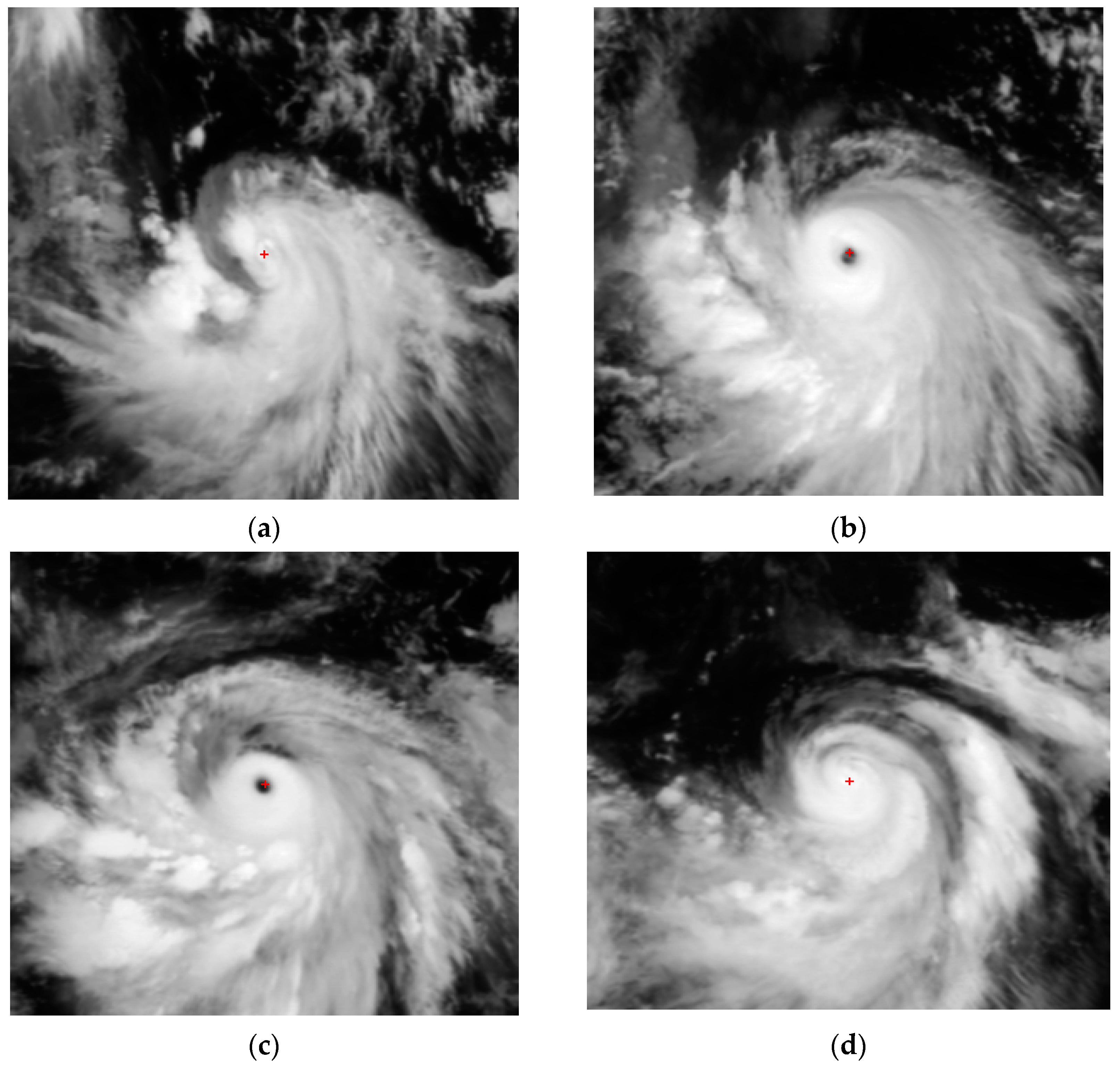
In this section, a case study of two TCs named Halong and Rammasun, which formed in the northwest Pacific in 2014, were selected to evaluate the effectiveness of the proposed algorithm. A total of 1000 FY-2E IR sequence images with half hour intervals were used to construct the cloud wind field and detect the center of the TCs. Some previously proposed algorithms have good positioning effects on the TC center in the mature stage, and the effects of the formation and dissipation phase are insignificant. The TC was selected from Halong for the case study in this section. As shown in Figure 2, the red “+” symbol was the center of the TC. Figure 2a,d is the TC in the formative period and the dissipation stage, respectively, which had no obvious TC eye compared with the mature stage. Figure 2b,c is the TCs in their mature stages, which have formed the obvious TC eye. It could be seen from Figure 2 that the center of the TC was detected accurately in the whole life cycle of the TC using the proposed algorithm.

3.2. Validation Method

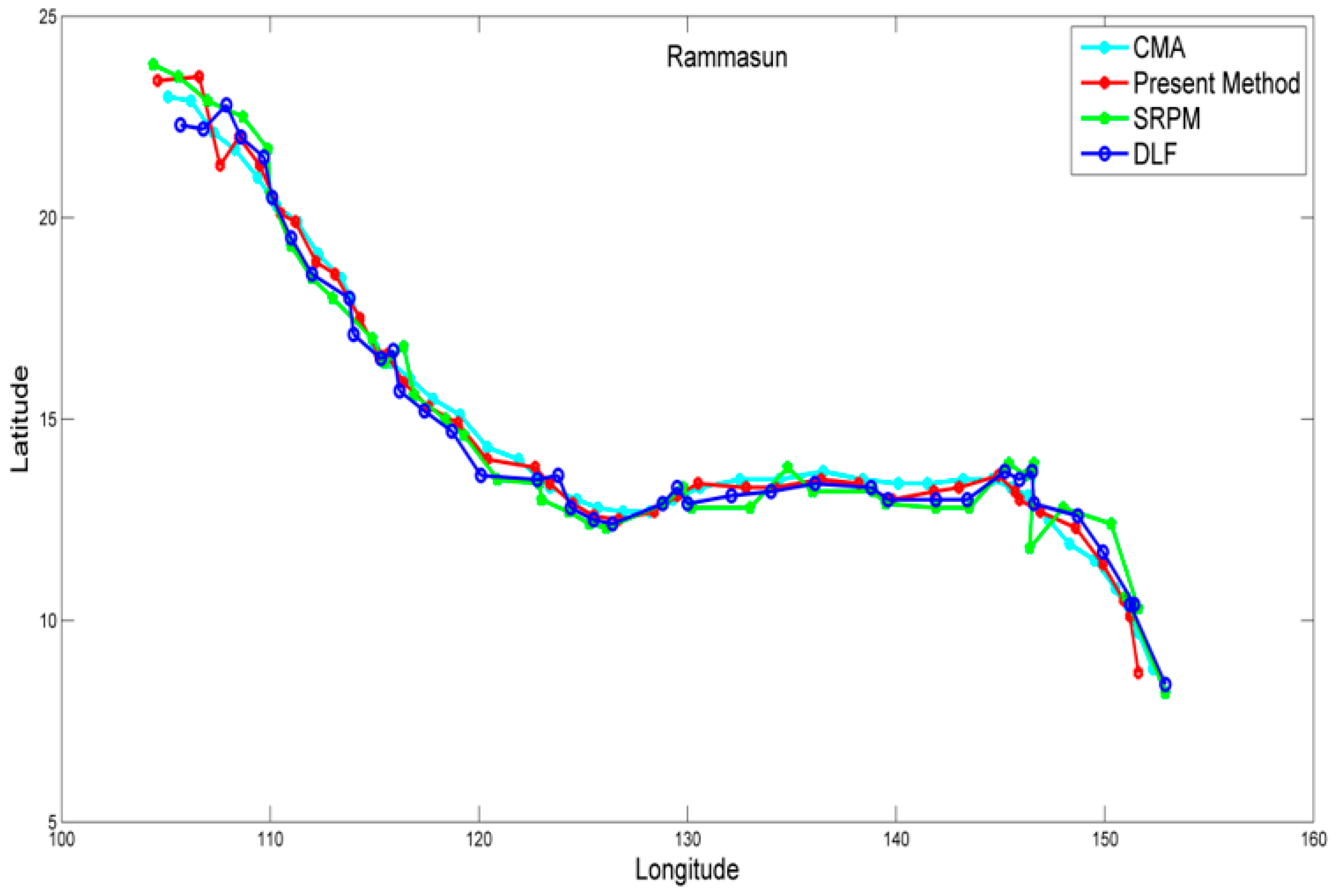
Super TC Rammasun was the ninth named storm in the Pacific TC season in 2014, causing serious damage to Hainan, Guangdong and Guangxi in China. The storm formed in the northwest Pacific Ocean on 10 July 2014 and had a maximum wind speed of over 17 classes (72 m/s). Rammasun was the strongest TC and caused landfalls in southern China for 41 years, and it dissipated on 21 July 2014. From 10 July 2014, 0000UTC to 19 July 2014, 1800UTC, approximately 400 FY-2E IR image sequences were processed and the center of the TCs were identified. The tracking results for the center of Rammasun along with a comparison of the CMA, SRPM [17] and DLF [24] methods are illustrated in Figure 3. It could be seen that the proposed algorithm produced the tracking results of the best path, which were quite close to the optimal path of CMA. The average tracking error of the proposed algorithm was approximately 41.76 km, and that of the SRPM and DLF methods were about 46.52 km and 41.83 km, respectively; thus it could be observed that the error of the proposed algorithm was smaller.

Super TC Halong was formed in the sea near Chuuk on 26 July 2014. The joint TC warning center upgraded it to a tropical storm. Halong was strengthened into a strong TC at 0800UTC on 2 August, and dissipated at 2000UTC on 11 August. From 2330UTC on 27 July 2014 to 0630UTC on 10 August 2014, six hundred and thirty-eight IR image sequences were chosen to evaluate this method. The center of each TC was determined using the proposed method. The comparison between the tracking results of Halong’s center along with the CMA, SRPM and DLF methods is given in Figure 4. It could be observed that the tracking results of the proposed algorithm were closest to the optimal path of CMA. The average tracking error of the proposed algorithm was about 41.92 km, and the error of the SRPM and DLF methods were about 45.31 km and 41.97 km, respectively; therefore, the error of the proposed algorithm was smaller.

Super TC Haiyan was formed on 3 November 2013 and was the strongest tropical cyclone in the world in 2013. The TC gradually intensified and became a super strong TC on 7 November 2013. From 0600UTC on 3 November 2013 to 1200UTC on 11 November 2013, approximately 360 FY-2E IR images sequences were processed and the centers of the TCs were identified. The tracking results for the center of Haiyan along with the comparison of the CMA, SRPM and DLF methods are illustrated in Figure 5. It could be seen that the proposed algorithm was tracking results of the best path that were quite close to the optimal path of CMA. The average tracking error of the proposed algorithm was around 40.85 km, and that of the SRPM and DLF methods were about 43.72 km and 40.91 km, respectively; thus it could be observed that the error of the proposed algorithm was smaller than other similar methodologies.

4. Conclusions

A novel objective algorithm named CMW was developed for detecting a TC’s center. A cloud motion wind-based detecting method was developed to fix a TC center using satellite infrared image sequences. The optical flow model with weighted median filtering was introduced to build a cloud motion wind field, and the density matrix method was utilized to calculate a TC’s center. Three super TCs, Halong, Rammasun and Haiyan, were analyzed using the proposed algorithm. The case studies demonstrated that the presented algorithm achieved satisfactory results in experiments and outperformed the SRPM and DLF methods. The average tracking error of the proposed algorithm was approximately 41 km, which was smaller than other similar methods, indicating that the proposed method is more efficient and reliable. Moreover, the ability of the CMW algorithm with good computational efficiency made it a desirable choice for TC forecasting. The present algorithm has the potential to be employed to assist forecasters to detect the track of an imminent TC and could even perform in a fully automated mode and provide objective identification of TC centers. In future work, a deep learning framework and salient region detection method will be introduced to improve detection accuracy in the analysis of centers of TCs.

References

- Jaiswal, N.; Kishtawal, C.M. Automatic determination of center of tropical cyclone in satellite generated ir images. IEEE Geosci. Remote Sens. Lett. 2011, 8, 460–463. [Google Scholar] [CrossRef]
- Chen, R.; Zhang, W.; Wang, X. Machine learning in tropical cyclone forecast modeling: A review. Atmosphere 2020, 11, 676. [Google Scholar] [CrossRef]
- Emanuel, K. 100 years of progress in tropical cyclone research. Meteorol. Monogr. 2018, 59, 15.1–15.68. [Google Scholar] [CrossRef]
- Roberts, M.J.; Camp, J.; Seddon, J.; Vidale, P.L.; Hodges, K.; Vanniere, B.; Mecking, J.; Haarsma, R.; Bellucci, A.; Scoccimarro, E.; et al. Impact of model resolution on tropical cyclone simulation using the HighResMIP–PRIMAVERA multimodel ensemble. J. Clim. 2020, 33, 2557–2583. [Google Scholar] [CrossRef] [Green Version]
- Zhang, G.; Murakami, H.; Knutson, T.R.; Mizuta, R.; Yoshida, K. Tropical cyclone motion in a changing climate. Sci. Adv. 2020, 6, eaaz7610. [Google Scholar] [CrossRef] [PubMed] [Green Version]
- Chaurasia, S.; Kishtawal, C.M.; Pal, P.K. An objective method of cyclone centre determination from geostationary satellite observations. Int. J. Remote Sens. 2010, 31, 2429–2440. [Google Scholar] [CrossRef]
- Fan, W.; Wang, X.; Wu, Y. Incremental graph pattern matching. ACM Trans. Database Syst. 2013, 38, 1–47. [Google Scholar] [CrossRef] [Green Version]
- Knaff, J.A.; DeMaria, R.T. Forecasting tropical cyclone eye formation and dissipation in infrared imagery. Weather Forecast. 2017, 32, 2103–2116. [Google Scholar] [CrossRef]
- Zheng, G.; Yang, J.; Liu, A.K.; Li, X.; Pichel, W.G.; He, S. Comparison of typhoon centers from SAR and IR images and those from best track data sets. IEEE Trans. Geosci. Remote Sens. 2016, 54, 1000–1012. [Google Scholar] [CrossRef]
- Liu, J.N.K.; Feng, B.; Wang, M.; Luo, W. Tropical cyclone forecast using angle features and time warping. In Proceedings of the 2006 IEEE International Joint Conference on Neural Network (IJCNN), Vancouver, BC, Canada, 16–21 July 2006; pp. 4330–4337. [Google Scholar]
- Wong, K.Y.; Yip, C.L.; Li, P.W. A novel algorithm for automatic tropical cyclone eye fix using Doppler radar data. Meteorol. Appl. 2007, 14, 49–59. [Google Scholar] [CrossRef]
- Yurchak, B.S. Description of cloud-rain bands in a tropical cyclone by a hyperbolic-logarithmic spiral. Russ. Meteorol. Hydrol. 2007, 32, 8–18. [Google Scholar] [CrossRef]
- Hawkins, J.D.; Turk, F.J.; Lee, T.F.; Richardson, K. Observations of tropical cyclones with the SSMIS. IEEE Trans. Geosci. Remote Sens. 2008, 46, 901–912. [Google Scholar] [CrossRef]
- Piñeros, M.F.; Ritchie, E.A.; Tyo, J.S. Objective measures of tropical cyclone structure and intensity change from remotely sensed infrared image data. IEEE Trans. Geosci. Remote Sens. 2008, 46, 3574–3580. [Google Scholar] [CrossRef]
- Jaiswal, N.; Kishtawal, C.M. Objective detection of center of tropical cyclone in remotely sensed infrared images. IEEE J. Sel. Top. Appl. Earth Obs. Remote Sens. 2013, 6, 1031–1035. [Google Scholar] [CrossRef]
- Thatcher, L.; Takayabu, Y.N.; Yokoyama, C.; Pu, Z. Characteristics of tropical cyclone precipitation features over the western Pacific warm pool. J. Geophys. Res.-Atmos. 2012, 117, 1–12. [Google Scholar] [CrossRef]
- Jin, S.; Wang, S.; Li, X.; Jiao, L.; Zhang, J.A.; Shen, D. A salient region detection and pattern matching-based algorithm for center detection of a partially covered tropical cyclone in a SAR image. IEEE Trans. Geosci. Remote Sens. 2017, 55, 280–291. [Google Scholar] [CrossRef]
- Creasey, R.L.; Elsberry, R.L. Tropical cyclone center positions from sequences of HDSS sondes deployed along high-altitude overpasses. Weather Forecast. 2017, 32, 317–325. [Google Scholar] [CrossRef]
- Wimmers, A.J.; Velden, C.S. Advancements in objective multisatellite tropical cyclone center fixing. J. Appl. Meteorol. Climatol. 2016, 55, 197–212. [Google Scholar] [CrossRef]
- Nguyen, L.T.; Molinari, J.; Thomas, D. Evaluation of tropical cyclone center identification methods in numerical models. Mon. Weather Rev. 2014, 142, 4326–4339. [Google Scholar] [CrossRef]
- Park, M.S.; Kim, M.; Lee, M.I.; Im, J.; Park, S. Detection of tropical cyclone genesis via quantitative satellite ocean surface wind pattern and intensity analyses using decision trees. Remote Sens. Environ. 2016, 183, 205–214. [Google Scholar] [CrossRef]
- Smith, R.K.; Kilroy, G.; Montgomery, M.T. Tropical cyclone life cycle in a three-dimensional numerical simulation. Q. J. R. Meteorol. Soc. 2021, 147, 3373–3393. [Google Scholar] [CrossRef]
- Hu, Y.; Zou, X. Comparison of Tropical Cyclone Center Positions Determined from Satellite Observations at Infrared and Microwave Frequencies. J. Atmos. Ocean. Technol. 2020, 37, 2101–2115. [Google Scholar] [CrossRef]
- Hu, Y.; Zou, X. Tropical Cyclone Center Positioning Using Single Channel Microwave Satellite Observations of Brightness Temperature. Remote Sens. 2021, 13, 2466. [Google Scholar] [CrossRef]
- Kim, M.; Park, M.S.; Im, J.; Park, S.; Lee, M.-I. Machine learning approaches for detecting tropical cyclone formation using satellite data. Remote Sens. 2019, 11, 1195. [Google Scholar] [CrossRef] [Green Version]
- Hu, T.; Wu, Y.; Zheng, G.; Zhang, D.; Zhang, Y.; Li, Y. Tropical cyclone center automatic determination model based on HY-2 and QuikSCAT wind vector products. IEEE Trans. Geosci. Remote Sens. 2018, 57, 709–721. [Google Scholar] [CrossRef]
- Nair, A.; Srujan, K.S.S.S.; Kulkarni, S.R.; Alwadhi, K.; Jain, N.; Kodamana, H.; Sandeep, S.; John, V.O. A deep learning framework for the detection of tropical cyclones from satellite images. IEEE Geosci. Remote Sens. Lett. 2021, 19, 1–5. [Google Scholar] [CrossRef]
- Mayers, D.; Ruf, C. Tropical cyclone center fix using CYGNSS winds. J. Appl. Meteorol. Climatol. 2019, 58, 1993–2003. [Google Scholar] [CrossRef]
- Yang, H.; Wu, L.; Xie, T. Comparisons of four methods for tropical cyclone center detection in a high-resolution simulation. J. Meteorol. Soc. Jpn. Ser. II 2020, 98, 379. [Google Scholar] [CrossRef] [Green Version]
- Wang, P.; Wang, P.; Wang, C.; Yuan, Y.; Wang, D. A Center Location Algorithm for Tropical Cyclone in Satellite Infrared Images. IEEE J. Sel. Top. Appl. Earth Obs. Remote Sens. 2020, 13, 2161–2172. [Google Scholar] [CrossRef]
- Liu, J.; Liu, C.; Wang, B.; Qin, D. A novel algorithm for detecting center of tropical cyclone in satellite infrared images. In Proceedings of the 2015 IEEE International Geoscience and Remote Sensing Symposium (IGARSS), Milan, Italy, 26–31 July 2015; pp. 917–920. [Google Scholar]
- Sun, D.; Roth, S.; Black, M.J. Secrets of optical flow estimation and their principles. In Proceedings of the 2010 IEEE Conference on Computer Vision and Pattern Recognition (CVPR), San Francisco, CA, USA, 13–18 June 2010; pp. 2432–2439. [Google Scholar]
- Sun, D.; Roth, S.; Black, M.J. A quantitative analysis of current practices in optical flow estimation and the principles behind them. Int. J. Comput. Vis. 2014, 106, 115–137. [Google Scholar] [CrossRef] [Green Version]
Figure 1.
Illustration of the motion field. (a) IR image at 1730 UTC on 3 August 2014; (b) IR image at 1800 UTC on 3 August 2014; (c) motion field calculated using the proposed method.
Figure 2.
Center of the TC calculated using the proposed method. (a) IR image at 0530 UTC on 1 August 2014; (b) IR image at 0600 UTC on 2 August 2014; (c) IR image at 0000 UTC on 3 August; (d) IR image at 1830 UTC on 4 August.
Figure 3.
Comparison of different methods for Rammasun.
Figure 4.
Comparison of different methods for Halong.
Figure 5.
Comparison of different methods for Haiyan.