
Air Pollutants over Industrial and Non-Industrial Areas: Historical Concentration Estimates
by
 , , and
Jiri Michalik
1, 
Ondrej Machaczka
1,
Vitezslav Jirik
1,2,*,
Tomas Heryan
1,3 and
Vladimir Janout
1 1
Centre for Epidemiological Research, Faculty of Medicine, University of Ostrava, 703 00 Ostrava, Czech Republic
2
Department of Epidemiology and Public Health, Faculty of Medicine, University of Ostrava, 703 00 Ostrava, Czech Republic
3
Department of Finance and Accounting, School of Business Administration, Silesian University, 733 40 Karviná, Czech Republic
*
Author to whom correspondence should be addressed.
Atmosphere 2022, 13(3), 455; https://0-doi-org.brum.beds.ac.uk/10.3390/atmos13030455
Submission received: 31 January 2022
/
Revised: 7 March 2022
/
Accepted: 9 March 2022
/
Published: 11 March 2022
(This article belongs to the Special Issue Urban Air Chemistry in Changing Times)
Abstract
:Only a few researchers have addressed the issue of lifetime exposure related to air pollutant concentration. This study aims to develop a methodology to obtain the most reliable estimates of historical concentrations of air pollutants, which would be further applied to the long-term exposure evaluation. In particular, PM10, PM2.5, NO2, SO2, benzene, and B(a)P concentrations have been obtained. Data of monitored concentrations, model calculations, and subsequent implementation of several corrections based on previous work on temporal and spatial correlations of these substances in the air have been deployed. This work makes an original contribution to the field of meteorology and epidemiology because of this innovative technique to estimate the most reliable historical concentrations of air pollutants. The novelty of our work lies in the additional implications of this study because historical concentration data serve as input data for the construction of epidemiological associations. The approach is based primarily on the availability of monitoring results of air pollutants.
1. Introduction
Some of the highest concentrations of air pollutants within the European Union are found in the Czech Republic (CZ) [1] particularly in the Upper Silesian Metropolitan Area (currently shared with Poland) in the Moravian-Silesian Region hereafter referred to as the industrial area (IA), which is considered to be a polluted area. At the same time, there are other localities in the CZ. In contrast to the previous location, IA, these other areas can be described as an environmentally unpolluted, non-industrial area (NA), by which we mean an area with low concentrations of air pollutants (WHO global air quality guidelines: particulate matter (PM2.5 and PM10), ozone, nitrogen dioxide, sulphur dioxide and carbon monoxide (2021): https://apps.who.int/iris/handle/10665/345329 (accessed on 25 February 2022)). Consequently, one of the goals of the HAIE project (in acknowledgement) is to detect and quantify exposure to air pollutants over an extended period.
The aim of this study is to develop a methodology to obtain the most reliable estimates of historical concentrations of air pollutants, which could be further applied to the evaluation of long-term exposure. In particular, PM10, PM2.5, NO2, SO2, benzene, and B(a)P concentrations have been used. In addition to the description of the methodology, the required output was the historical time series of the average annual concentrations of the monitored pollutants related to the level of smaller territorial units(districts) of the compared areas IA and NA (The upper LAU level (LAU 1)—formerly NUTS 4—is defined only for the following countries: Cyprus, Czech Republic, Estonia, Finland, Greece, Hungary, Ireland, Latvia, Lithuania, Luxembourg, Malta, Poland, Portugal, Slovenia, Slovakia, and the United Kingdom (The Czech Statistical Office, https://www.czso.cz/csu/czso/1-1373-05--uvod (accessed on 25 February 2022))). These data will then serve as source data for the subsequent evaluation of the relationship between exposures and the biological effects of air pollution in the population studied. Another objective of the present work is the general comparison of the methodology of the specifically created procedure to obtain historical concentrations with the standard methodology currently in use. The possibility of obtaining an estimate of historical concentrations using dispersion modelling and its subsequent validation was not realistic, as the necessary input data (emissions and technical operational parameters of individual sources, adequately structured meteorological data, etc.) are not available in the evaluated historical horizons. As a result, these data have not been recorded and evaluated in the CZ in the past.
The most commonly used methodology to estimate concentration is land use regression (LUR) modelling [2]. LUR is based on the principle that the concentration of pollutants in any location depends on the environmental characteristics of the environment, especially those that affect or reflect the intensity of the emission and the efficiency of dispersion [2]. This approach requires a large amount of data that can influence concentration estimates, which are difficult or even impossible to obtain for historically distant time horizons. The LUR approach does not appear to us to be an appropriate methodology for achieving our objectives for the reasons described (see Section 3.2).
There are two basic (extreme) procedures for modelling and identifying real entities [3]. The first is the analytical procedure. The procedure is based on material and energy balances of the phenomenon (entity in this case) and knowledge of physical, chemical or. biological sub-processes taking place in it and their mathematical description. By applying this knowledge, we obtain an analytical (mathematical) model of the entity. This model describes the internal state variables of the modelled process and their interrelationships. The state quantities and parameters of the model have a specific physical significance. The resulting model is a model of the structure of the entity. It is called the internal model, but more often the state model of the entity. This model then captures the behaviour of the entity (system) [3]. We can also include the LUR methodology in this group.
The second basic procedure for identifying a real entity is the empirical procedure [3,4]. It is based on the measurement of input and output quantities in a real entity and their subsequent processing and evaluation. The product is then an experimental model of the real entity. This model does not describe the internal connections in the investigated entity; it bypasses internal state variables. It is not a model of the structure; it is only a model of behaviour. Its parameters are not specific physical significance. Because it only lists the relationship between input and output, it has the character of an external (input–output) model. This procedure is also used in our case.
Each of the two methods has its field of application and advantages. The analytical procedure is irreplaceable in the stage of prediction when, for various reasons, we need to estimate the future properties of the process, the state. The state model obtained by the analytical procedure is valid in a wide range of changes in input quantities, even in modes that are unacceptable (e.g., for safety reasons). Since its parameters have a specific physical significance, we can examine their influence on the outcome of the process. The disadvantage of this model is mainly its complexity and difficulty in building it, especially for more complex processes.
The empirical procedure logically requires the existence of a real entity (we perform measurements on it). In the field of measurement, for which the identification process took place, the experimental model may be more accurate than the model obtained analytically because the measurement results include those aspects of reality that we are not able to capture or neglect in analytical modelling. On the other hand, the model is valid only for this area of measurement, and for another area of changes (movement) of input quantities, we must compile a different model. The experimental model is usually much simpler than the analytical model. The methodological procedure we present for estimating historical concentrations has been adapted to the main objective and the availability and type of input data for each stage of the estimation. The originality of this methodology lies mainly in the fact that it uses empirical data on air pollutant concentration in the form of monitoring time series and their correlation with spatially modelled data [5], which could be simplistically described as ‘identification modelling’. The data obtained are thus further processed by a deeper historical correlation estimation using emission balance data. In this case, identification modelling is more appropriate than the LUR methodology, which is more suitable for estimating concentrations in terms of the spatial distribution in pollutants of the present state or for their prediction. For estimating historical concentrations, the effectiveness of the LUR methodology is suitable only for recent history for the reasons mentioned above. Therefore, the methodology we have developed is original in its use of available data of air pollutant concentrations of varying range and quality in combination with the geographic information system (GIS) tools and emission data. Furthermore, the proposed methodology for estimating concentration over long periods can be used for any population-based or analytical epidemiological studies dealing with chronic diseases, such as cardiovascular, respiratory, and oncological diseases.
2. Materials and Methods
2.1. Selection of Monitored Localities
The proposed methodology was applied in the CZ. The Moravian-Silesian region of the CZ (MS region or part of it), which lies in the northeast part of the country, can be considered as an industrial area, IA (see Figure 1).
The Moravian-Silesian Region is defined by the districts of Bruntál (BR), Frýdek-Místek (FM), Karviná (KA), Nový Jičín (NJ), Opava (OP), and Ostrava (OV) (see Figure 1). Since the 19th century, the region has been and is still one of the most important industrial regions of Central Europe [6]. OV is the capital of the IA region. The OV region and its surroundings have long been one of the most polluted areas not only in the CZ but also in Europe [1]. However, it is not clear whether the entire region or some part of it can be considered an industrial or environmentally polluted region. Due to this uncertainty, we processed data for the entire MS region, which can then be modified to individual districts. What is certain is that the allowed limits of air pollutants in this region [1] are regularly exceeded due to the concentration of pollution sources and the geological and meteorological conditions of Upper Silesia, where most of the region belongs. The main sources of pollution in most of the region are industry and energy, local heating, and road traffic. The region has abundant mineral reserves, especially coal, which has historically led to the introduction of large-scale heavy industry, especially primary metallurgy, steel and coke production, and the chemical industry [7]. Although this industry is currently in decline, as mentioned above, the area is still one of the most polluted, and environmental recovery will take a very long time.
The South Bohemia region, located in the southern part of the country, was chosen as a non-industrial area (NA non-industrial area). The South Bohemian Region is defined by the districts of České Budějovice (CB), Český Krumlov (CK), Jindřichův Hradec (JH), Písek (PI), Prachatice (PR), Strakonice (ST), and Tábor (TA) (see Figure 1). CB is the capital of the NA region. For a long time, it has been an agricultural area with developed fish farming and forestry. Only in the last century has the industry developed with a focus on manufacturing activities. Industrial production is concentrated mainly in the CB agglomeration. Compared to the IA region, this region is not a resource-rich area and contains almost no sources of raw energy materials. Therefore, the environment is characterized as less damaged and polluted [8]. The sources of pollution are mainly agriculture, but also industry, local heating, and automobile transport are contributing factors.
2.2. Input Data
The following air quality databases and relevant spatial characteristics were used as input data sources:
- a.
- Air quality monitoring data—Publicly available tabular summaries of data from air quality monitoring stations from a nationally verified air quality database [9].
- b.
- Publicly available five-year average concentrations according to the Air Protection Act 201/2012 Coll., 11, paragraphs 5 and 6 for the interval 2007–2011 in shapefile format (SHP)—A regular grid of squares with 1 km step [10].
- c.
- Boundaries of the IA and NA districts in the SHP format [11].
- d.
- Areas of built-up areas of shapefile districts in shapefile format of shapefiles (SHP) [11].
- e.
- Emission balance of assessed districts for the years 1980–1997 for PM, NOx, and SO2 from data processed by the Czech Hydrometeorological Institute in Prague (CHMI).
2.3. Data Processing
The proposed methodology consists of the following consecutive steps, corresponding to the following sections:
- i.
- Processing of available air quality monitoring data for individual districts and assessed pollutants: tabular overviews of data from air quality monitoring stations.
- ii.
- Creation of a corresponding database of five-year average concentrations of pollutants evaluated in the SHP format (regular network of squares with a step of 1 km) and preparation of digital map data in GIS, territorial identification of the evaluated area, and built-up area.
- iii.
- Calculation of annual average concentrations from air quality monitoring data and a database of average concentrations over five years.
- iv.
- Calculation of average annual concentrations of territorial units where air quality monitoring data were not available. Correlation of data explored in Steps i, ii, and iii.
- v.
- Correction of the annual average concentrations of territorial units for residential zones.
- vi.
- Estimation of the average annual concentrations of territorial units using the emission balance database for historical periods for which air quality monitoring data were not available.
2.3.1. Processing of Air Quality Monitoring Data
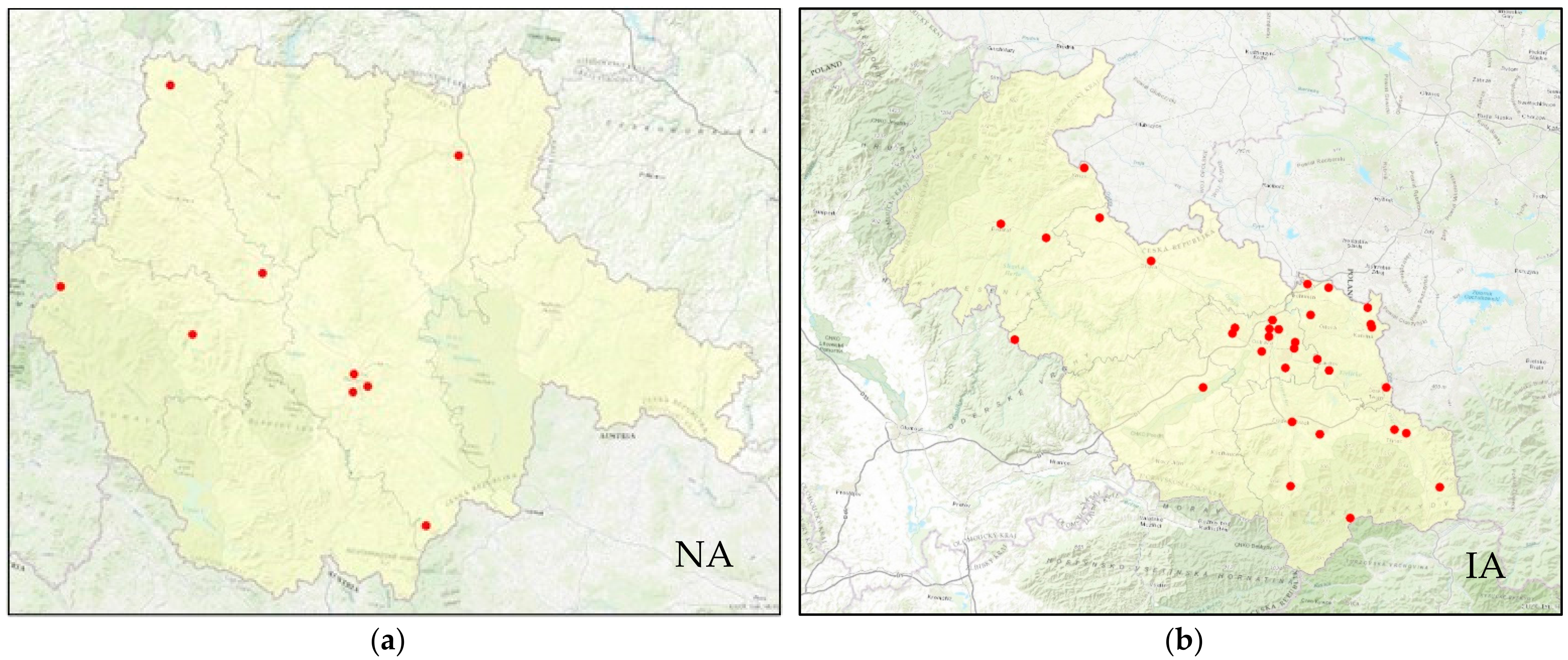
Air quality monitoring was first processed. Air quality monitoring data for both compared areas have been available in the database since 1997 (in the case of the OV district since 1972). The air quality monitoring station network meets the quality system requirements of the international standard EN ISO/IEC 17025:2017. In IA, compared to NA, the air quality monitoring network is significantly denser and the databases contain more monitored pollutants. Since 1997, there have been numerous changes in the location of air quality monitoring stations and their measurement programs. Figure 2 shows the location of air quality monitoring stations within the study areas as of 2019.
As a result of this disproportion, the data sets of the compared districts differed in terms of spatial sampling and the type of pollutants measured. Therefore, it was necessary to select a procedure to determine annual average district concentrations that could eliminate this as much as possible. Therefore, the air quality monitoring data were processed in the form of annual average concentrations for the available year and the pollutant of interest. Table 1 and Table 2 show the frequency of available values for annual average concentrations of individual air quality monitoring stations within districts compared for the entire period 1997–2019. The tables show the disparity of available data for individual districts compared districts and, in particular, between the assessment areas.
2.3.2. Application of the Spatial Database and Maps of Territorial Identification
The obtained values for annual average concentrations had to be adapted to the entire district area to eliminate the availability and disproportion of the concentration data. This was completed in the next step using the Database of Spatial Five-Year Average Annual Concentrations of Air Pollutants (according to the Air Protection Act 201/2012 Coll., 11, Paragraphs 5 and 6).
This database contains average values of pollutant concentrations for a square region with an area of 1 km2, always over five calendar years. These data are published annually by the Ministry of Environment for the entire CZ territory. The first database processed in this way is available for the period 2007–2011, which was also used in this step, because it lies in the middle of the range of available air quality monitoring data within the entire period 1997–2019. Figure 3 shows a sample of the spatial database of the five-year annual average for PM10 for the period 2007–2011. According to the needs of the proposed methodology, digital map layers in GIS format (boundaries of administrative units of the territory of the Czech Republic) were downloaded from the COSMC (Czech Office for Surveying, Mapping and Cadastre) Geoportal for further processing of the spatial database and also for graphic presentation purposes. From the data, only territorial units (including territorial identification codes) were used regarding the application of the methodology and were adequately simplified for these needs. The same source was used for obtaining GIS data with building entities, INSPIRE theme Buildings (BU), to define the built-up area.
2.3.3. Calculation of Annual Average Concentrations
To explore these annual average concentrations, it is followed by the calculation described by Equation (1):
where CcA means corrected annual average concentrations, also including historical concentrations within the entire period 1997–2019 of each pollutant for each year attributed to the particular district where air quality monitoring data were available. Variable CmRP stands for those annual average concentrations (via Section 2.3.1) from air quality monitoring data m in a particular district and each correlated pollutant P for a given year R. Both CmRP and CmRPi are explored through the interval averages for the i period 2007–2011, and together means the correction to explore CcA. Finally, the variable CRP is then the average annual concentration from the database of spatial five-year concentrations for the monitored pollutant calculated from the data at the points of the regular network using GIS tools (ArcGIS Pro).
CcA = CmRP/(CmRPi/CRP)
The next step was to obtain the CcA values for pollutants for years when air quality monitoring data were not available at all or were available only for some pollutants in some districts and years. This was mainly because the monitoring was not carried out at all or did not last long enough to be interpreted as annual average concentrations (see Table 1 and Table 2). The CcA values already obtained formed the basis for filling in the missing data based on correlations between individual pollutants in the districts. The correlation coefficients were determined for each district from the CRP averages between the pollutants. If some districts did not have data for the correlation calculation, concentrations were determined from data with similarly burdened districts in the assessment area. The corresponding concentration of a similar district (based on the character of the urban landscape and the relative geographic location) was corrected according to Equation (2):
where KdRP is the ratio of the values of the regular grid points for a given year (R) and each correlated pollutant (P). Symbols a and b are two different relevant pollutants representing particularly correlations of PM10 with PM2.5 and B(a)P, as well as the correlation with NO2 used to calculate benzene. Strong associations were found between these pollutants [12,13]. Following the above procedure, all annual average district concentrations for monitored pollutants were calculated for the period 1997–2019.
KdRP = CRPa/CRPb
2.3.4. Correction of Annual Concentrations to Residential Zones
Since annual average concentrations for the district serve as a basis for evaluating the exposure of the population to individual pollutants, it was necessary to correct annual average concentrations for the entire district to residential zones. The rationale is to use the established district concentrations for their subsequent use in determining population exposures. For this purpose, data on the boundaries of the IA and NA districts and the area of the built-up areas of the districts were used in the SHP format.
A correction was made using GIS and statistics. A polygonal layer defining residential zones was used to select regular grid points for each district and pollutant (Spatial Five-Year Average Concentration Database 2007–2011), from which basic statistical indicators (arithmetic mean, median, lower, and upper quartile) were calculated. The same statistical indicators were also evaluated for all points in the district network. The concentration adjustment factors for residential areas (KRA) were determined as the ratio of the median residential area to the entire district area. These districts and the corresponding pollutants were corrected if the value of the median ratio was outside the interval (0.95–1.05). Overall, the correction in terms of residential zones was made in 24 cases out of 78 possible cases (13 districts and six pollutants assessed). The lowest value of the correction was 0.88 and the largest was 1.28. The correction was applied in 9 cases in NA and 15 cases in IA, with the most frequent being for B(a)P.
2.3.5. Estimation of Concentrations for the Years 1980–1997 Using Data from Annual Emission Balances of Assessed Districts
In the next step, estimates of district concentrations for the period 1980–1995 were made. In this case, it is only an estimate and, for this purpose, the National Emission Inventory (CLRTAP) for the whole district and its subsequent correlation with air quality monitoring data were used. Data from the OV district were used for the basic correlation calculation, for which air quality monitoring data for a suspended particular matter and sulphur dioxide were available until 1972. Conversion to average annual district concentrations and calculation of other pollutants until 1980 (last available emission data) in the first step was performed retrospectively for the OV district in the same way as for the period 1997–2019. The following graph (Figure 4) shows the basic data of the OV district and their trends for 1980, 1985, 1990, and 1995, which were used to calculate the concentration data of other districts. The determination of concentrations until 1980 used a direct proportion between available concentrations and the emission balance.
Due to the greater uncertainty and some variability in the emission data, these air pollutant concentration data estimates were made at five-year intervals only for the years 1980, 1985, 1990, and 1995, with 1997 as the last follow-up year that was processed using a more accurate method for the interval 1997–2019. Therefore, for the period 1980–1995, the data for the districts were estimated from the correlation trends of the ‘emission data versus air pollutant concentration data’ of the OV district, assuming a similar trend for all districts and continuity with 1997. The benchmark for the IA region was the OV district and for the NA region the CB district because both districts showed similar trends in terms of air pollutant concentration data in the years 1997–2019, as can be seen in the following two graphs (Figure 5 and Figure 6).
The first calculation was the estimation of the air pollutant concentration of the CB district for 1980, which was based on the direct proportion of the ratio of the air pollutant concentration and emission characteristics of the OV district and the calculated district (CB), where the unknown calculated is the air pollutant concentration for 1980. This was performed for PM10, NO2, and SO2 concentrations. The values of the concentrations of these three pollutants between 1980 and 1997 were interpreted the same way as the data presented in Figure 4—trends in the concentration of air pollutants for the OV district for the years 1980–1997. The PM2.5 concentration (KPM2.5) was derived from the correlation of PM10 and PM2.5 based on the trends shown in Figure 4 above.
KPM2.5 = PM2.5/PM10 = 0.77
In the case of benzene and B(a)P concentrations, it was assumed that for the time interval 1980–1995 the concentrations of these two pollutants would be identical to 1997 due to the large uncertainty in the estimates. In this way, air pollutant concentrations were determined for all NA and IA assessment districts. These data were then corrected for built-up areas using the same method as for the period 1997–2019.
3. Results and Discussion
3.1. Example of the Results of the Described Methodology for Estimating Historical Air Pollutant Concentrations
The resulting annual concentration data for each year under consideration consist of a total of 78 values (six pollutants for the 13 districts assessed). For the period 1997–2019, the total number of years was 23. For the period 1980 to 1997, the total number of estimated years was four (five-year intervals 1980, 1985, 1990, and 1995). Due to the large size of the resulting dataset, the results are presented in this study as an example in the form of comparison maps between IA and NA for PM10 and only for the years 1980, 1997, and 2019 (Figure 7, Figure 8 and Figure 9). Figure 10 shows graphically the resulting time series of annual average PM10 concentrations of each district of the compared areas for the period 1980–2019. In this case, the determination of the estimated concentrations for all districts was based on the needs of the HAIE project, for which the concentrations were estimated. The entire procedure is focused on epidemiological studies, where population health data are related to the smallest territorial unit of the district.
The results must be divided into two parts, particularly the results of estimates for the period 1997–2019 and the period 1980–1995. This is mainly due to the accuracy of the calculated concentration estimates. For concentration estimation in the period 1997–1999, the uncertainty of the results from a spatial point of view is mainly influenced by the number of air quality monitoring stations in the respective district and their distribution within the territory of the district. In terms of the correlation between the individual pollutants assessed, the uncertainty is also affected by the number of pollutants monitored within individual air quality monitoring stations. In this case, the estimated values will be more valid in the industrially loaded districts of the Moravian-Silesian Region than in non-industrial districts and the South Bohemian region. The estimate of concentrations for the period 1980–1995 is burdened with more uncertainty than in the previous case. This is because the concentration estimate is directly related to the 1997 concentration estimates and uses correlations with emission balance data for the individual districts under consideration in combination with the concentration estimates for the OV district for the concentration estimate itself. The fact that the emission balances report data for the sum of PM and NOx is also uncertain.
Both methods of estimating concentrations are further affected by the uncertainty of the correction of the resulting concentrations to the populated zones of the districts. However, this uncertainty will be considerably lower than the previous uncertainties due to the values of the corrections used. After 1998, the concentrations more or less stabilized, and the further decline is not as pronounced. This is mainly because after 1989 there was a significant decline in heavy industry in the following 10 years—apparent in Figure 10 below—and the introduction of most BAT was made in 2000 (progressive separation of solid pollutants, separation of gaseous pollutants, hermeticization of coke oven battery operations, etc.).
3.2. Comparison of the Described Methodology for Estimating Historical Concentrations with the Standard Methodology Used
In other countries, land use regression (LUR) modelling is commonly used to estimate exposures [2]. LUR is based on the principle that the concentration of pollutants at any location depends on the environmental characteristics of the environment, in particular those that affect or reflect the intensity of emissions and the efficiency of dispersion. The modelling is performed by creating multiple regression equations that describe the relationship of the concentration between the measured concentrations in the sample of monitoring sites and the relevant environmental variables calculated by GIS for the zones of influence around each site. The resulting equation is then used to predict concentrations at unmonitored sites based on prediction variables. Prediction can be made for specific point locations (e.g., residential building addresses) or a fine grid; in the latter case, a raster map of the study area can be created, which intersects with the population data at the area level behind the exposure distribution estimate. Geographically localized air quality monitoring data are necessary inputs for the construction of the LUR model. However, these data are often limited by the scope and configuration of the available national, regional, and local monitoring networks. LUR was originally developed as a means of assessing concentrations of traffic-related air pollution. The LUR assumes monitoring data for 30–40 stations, which we do not have for each assessment year. These data should relate to primary factors and processes affecting pollutant concentrations, such as the distribution and intensity of the emission source (e.g., road length, traffic intensity, emission balance of industrial zones), and dispersion efficiency (e.g., altitude, wind speed, surface roughness) [16,17]. In addition, we did not have emission data for individual emission sources and their locations, but only aggregated emissions for the entire sub-area.
When comparing our specific methodological procedure for estimating concentration with the LUR method, we can state the following.
- Both procedures require GIS as a necessary tool to achieve their results.
- Unlike LUR, it is not possible to use this procedure correctly for forward-looking concentration predictions. It is suitable for estimating historical concentrations from available air quality monitoring data for the entire area of interest.
- Compared to the proposed approach, the LUR method requires a larger number of monitoring stations with a sufficiently variable number of characteristic types of monitored zones. In our case, we use a specific long-term average regular network of the air pollution characteristics database for estimation, which serves as a spatially very detailed basis for identification modelling from available air quality monitoring data.
- Unlike the LUR method, it is not necessary to define other variables, such as the distribution and intensity of emission sources and elements of pollutant efficiency, the definition of which introduces additional uncertainties into the prediction. These parameters are taken into account much more accurately by identification with the regular network of the air pollution characteristics database.
- Compared to LUR, the air quality monitoring data used in combination with the spatial database of air pollution characteristics represent in the long run a more closely linked system in terms of time and space.
- In terms of the evaluated time horizons, the complexity of processing input data and the requirement to obtain average values at the territorial level of districts, the proposed procedure is more suitable than the LUR method.
4. Conclusions
This study aimed to develop a methodology to obtain the most reliable estimates of historical concentrations of air pollutants, which would be further applied to the long-term exposure evaluation. In particular, PM10, PM2.5, NO2, SO2, benzene, and B(a)P concentrations were obtained. Although it was necessary to deal with the insufficient or complete absence of input data or the different availability of input data between the areas compared, all these factors can lead to a certain degree of inaccuracy in some particular cases.
The meaning of determining and using historical concentrations may vary. In our case, the need for a solid estimate of long-term or lifetime exposures of the population led us to this. Such estimates are necessary when epidemiological studies on chronic diseases do not become apparent until several decades after birth and many, especially oncological diseases, need to relate to lifetime exposure to pollutants. Although estimating long-term or lifetime exposures from historical concentrations is only a partial part of epidemiological research, it has an irreplaceable role to play here. In several publications, chronic diseases have been precisely linked to exposure to pollutants, which have been obtained from estimates from measured data or models only in the last few years. However, if the assessed population lives in regions with large changes in pollutant concentrations or a strong trend in time series, then the results of such studies are subject to high uncertainties when assessing the relationships between exposures and their consequences. Our study has sought to find a way to reduce these uncertainties to the lowest possible level.
An important factor of the developed methodology is its limitation, which consists mainly in the availability of a database of average long-term concentrations of pollutants and their temporal and spatial distribution in the evaluated area. It may be obvious that solid estimates of historical concentrations can only be made using our methodology up to a certain smallest spatial unit and a certain historical time, which does not necessarily meet the needs of epidemiological research in all cases. Therefore, before applying this methodology, researchers must evaluate this aspect.
Author Contributions
Conceptualization, J.M. and V.J. (Vitezslav Jirik); methodology, J.M.; software, J.M.; validation, V.J. (Vitezslav Jirik); formal analysis, J.M. and T.H; investigation, O.M.; data curation, O.M.; writing—original draft preparation, O.M. and J.M.; writing—review and editing, V.J. (Vitezslav Jirik), J.M., T.H., and V.J. (Vladimir Janout); visualization, J.M., T.H., and O.M.; supervision, V.J. (Vitezslav Jirik) and V.J. (Vladimir Janout); project administration, V.J. (Vitezslav Jirik). All authors have read and agreed to the published version of the manuscript.
Funding
This research was supported by the European Regional Development Fund under Grant ‘Healthy Aging in Industrial Environment—HAIE’ (Grant No. CZ.02.1.01/0.0/0.0/16_019/0000798).
Data Availability Statement
Data are available from the corresponding author upon reasonable request.
Conflicts of Interest
The authors declare no conflict of interest.
References
- European Environment Agency. Air Quality in Europe—2019 Report; Publications Office of the European Union: Luxembourg, 2019; Available online: https://www.eea.europa.eu/publications/air-quality-in-europe-2019 (accessed on 24 September 2021). [CrossRef]
- Eeftens, M.; Beelen, R.; de Hoogh, K.; Bellander, T.; Cesaroni, G.; Cirach, M.; Declercq, C.; Dedele, A.; Dons, E.; de Nazelle, A.; et al. Development of land use regression models for PM2.5, PM2.5 absorbance, PM10 and PM coarse in 20 European study areas; Results of the ESCAPE project. Environ. Sci. Technol. 2012, 46, 11195–11205. [Google Scholar] [CrossRef] [PubMed]
- Dostal, P.; Gazdos, F. Řízení Technologických Procesu (Management of Technological Processes); Univerzita Tomáše Bati ve Zlíně: Zlin, Czech Republic, 2006; ISBN 8073184656. [Google Scholar]
- Kim, S.-Y.; Bechle, M.; Hankey, S.; Sheppard, L.; Szpiro, A.A.; Marshall, J.D. Concentrations of criteria pollutants in the contiguous U.S., 1979–2015: Role of prediction model parsimony in integrated empirical geographic regression. PLoS ONE 2020, 15, e0228535. [Google Scholar] [CrossRef] [PubMed] [Green Version]
- ESRI: ArcGIS Pro: Spatial Analysis in ArcGIS Pro. Available online: https://pro.arcgis.com/en/pro-app/latest/help/analysis/introduction/spatial-analysis-in-arcgis-pro.htm (accessed on 29 July 2021).
- Český Statistický Úřad. Krajská Správa ČSÚ v Ostravě: Charakteristika Moravskoslezského Kraje (Czech Statistical Office: Regional Administration of the CZSO in Ostrava: Characteristics of the Moravian-Silesian Region). Available online: https://www.czso.cz/csu/xt/charakteristika_moravskoslezskeho_kraje (accessed on 17 May 2021).
- Jirik, V.; Machaczka, O.; Miturová, H.; Tomasek, I.; Slachtova, H.; Janoutova, J.; Velicka, H.; Janout, V. Air pollution and potential health risk in ostrava region—A review. Cent. Eur. J. Public Health 2016, 24, S4–S17. [Google Scholar] [CrossRef] [PubMed] [Green Version]
- Český Statistický Úřad: Krajská Správa ČSÚ v Českých Budějovicích: Charakteristika Kraje (Czech Statistical Office: Regional Administration of the CZSO in České Budějovice: Characteristics of the Region). Available online: https://www.czso.cz/csu/xc/charakteristika_kraje (accessed on 17 May 2021).
- Czech Hydrometeorological Institute: Air Pollution and Atmospheric Deposition in Data, the Czech Republic: Annual Tabular Overview. Available online: https://www.chmi.cz/files/portal/docs/uoco/isko/tab_roc/tab_roc_EN.html (accessed on 1 May 2021).
- Český Hydrometeorologický Ústav: Pětileté Průměrné Koncentrace (Czech Hydrometeorological Institute: Five-Year Average Concentrations). Available online: https://www.chmi.cz/files/portal/docs/uoco/isko/ozko/ozko_CZ.html (accessed on 1 May 2021).
- Český Úřad Zeměměřický a Katastrální: Geoportál ČÚZK: Soubor Správních Hranic a Hranic Katastrálních Území ČR (Czech Surveying and Cadastre Office: CSCO Geoportal: A Set of Administrative Borders and Borders of Cadastral Territories of the Czech Republic). Available online: https://geoportal.cuzk.cz/(S(ep0r2vsgn1lfq0s4lfefnkwb))/Default.aspx?mode=TextMeta&side=dSady_RUIAN&metadataID=CZ-CUZK-SH-V&mapid=5&head_tab=sekce-02-gp&menu=25 (accessed on 1 May 2021).
- Fernández-Somoano, A.; Llop, S.; Aguilera, I.; Tamayo-Uria, I.; Martínez, M.D.; Foraster, M.; Ballester, F.; Tardón, A. Annoyance Caused by Noise and Air Pollution during Pregnancy: Associated Factors and Correlation with Outdoor NO2 and Benzene Estimations. Int. J. Environ. Res. Public Health 2015, 12, 7044–7058. [Google Scholar] [CrossRef] [PubMed] [Green Version]
- Sharma, R.; Sharma, N. Assessment of variations and correlation of ozone and its precursors, benzene, nitrogen dioxide, carbon monoxide and some Meteorological Variables at two sites of significant spatial variations in Delhi, Northern India. Pollution 2021, 7, 723–737. [Google Scholar] [CrossRef]
- Cernikovsky, L.; Krejci, B.; Blazek, Z.; Volna, V. Transboundary airpollution transport in the Czech-Polish Border Region between the cities of Ostrava and Katowice. Cent. Eur. J. Public Health 2016, 24 (Suppl.), 45–50. [Google Scholar] [CrossRef] [PubMed] [Green Version]
- Jancik, P.; Pavlikova, I.; Bitta, J.; Hladky, D. Atlas Ostravského Ovzduší; Vysoká Škola Báňská—Technická Univerzita Ostrava: Ostrava, Czech Republic, 2013; ISBN 978-80-248-3006-3. [Google Scholar]
- Land Use Regression. Integrated Environmental Health Impact Assessment System. Available online: http://www.integrated-assessment.eu/eu/guidebook/land_use_regression.html (accessed on 17 May 2021).
- Vienneau, D.; de Hoogh, K.; Beelen, R.; Fischer, P.; Hoek, G.; Briggs, D. Comparison of land-use regression models between Great Britain and the Netherlands. Atmos. Environ. 2010, 44, 688–696. [Google Scholar] [CrossRef]
Figure 1.
Localization of the compared regions and their districts within the Czech Republic.

Figure 2.
Location of air quality monitoring stations (red points) within the compared areas in 2019: (a) NA; (b) IA.
Figure 2.
Location of air quality monitoring stations (red points) within the compared areas in 2019: (a) NA; (b) IA.

Figure 3.
Sample spatial database—five-year average 2007–2011, PM10 (µg/m3) [10].
Figure 3.
Sample spatial database—five-year average 2007–2011, PM10 (µg/m3) [10].

Figure 4.
Trends in air pollutant concentration in the OV district 1980–1997.

Figure 5.
Trends in air pollutant concentration for the OV district for the years 1997–2019.

Figure 6.
Trends in air pollutant concentration for the CB district for the years 1997–2019.

Figure 7.
Example of the results of the described methodology—PM10 concentration for the year 1980.

Figure 8.
Example of the results of the described methodology—PM10 concentration for the year 1997.

Figure 9.
Example of the results of the described methodology: PM10 concentration for the year 2019.
Figure 9.
Example of the results of the described methodology: PM10 concentration for the year 2019.

Figure 10.
Example of the results of the described methodology: estimation of historical PM10 concentrations for monitored sites for the period 1980–2019.
Figure 10.
Example of the results of the described methodology: estimation of historical PM10 concentrations for monitored sites for the period 1980–2019.

Figure 11.
Comparison of emission and estimations of historical PM10 concentrations trends for the monitored sites in the year 1980.
Figure 11.
Comparison of emission and estimations of historical PM10 concentrations trends for the monitored sites in the year 1980.

Figure 12.
Comparison of emission and estimations of historical PM10 concentration trends for monitored sites in the year 1997.
Figure 12.
Comparison of emission and estimations of historical PM10 concentration trends for monitored sites in the year 1997.

Figure 13.
Comparison of emission and estimations of historical PM10 concentration trends for the monitored sites in the year 2019.
Figure 13.
Comparison of emission and estimations of historical PM10 concentration trends for the monitored sites in the year 2019.


Table 1.
Number of annual average concentrations available for IA in 1997–2019.
| IA Districts | PM10 | * PM2.5 | NO2 | SO2 | * B(a)P | * Benzene |
|---|---|---|---|---|---|---|
| BR | 7 | 4 | 9 | 13 | 3 | n/a |
| FM | 117 | 28 | 95 | 120 | 5 | 17 |
| KA | 154 | 38 | 173 | 170 | 31 | 11 |
| NJ | 36 | 8 | 31 | 38 | 8 | n/a |
| OP | 44 | 5 | 41 | 38 | 7 | 8 |
| OV | 360 | 54 | 230 | 364 | 92 | 112 |
* 1997–2018.
Table 2.
Number of annual average concentration values for NA in 1997–2019.
| NA Districts | PM10 | * PM2.5 | NO2 | SO2 | * B(a)P | * Benzene |
|---|---|---|---|---|---|---|
| CB | 64 | 14 | 53 | 56 | 16 | 14 |
| CK | n/a | n/a | n/a | 2 | n/a | n/a |
| JH | n/a | n/a | 6 | 16 | n/a | n/a |
| PI | n/a | n/a | n/a | 2 | n/a | n/a |
| PR | 38 | 6 | 42 | 37 | 1 | n/a |
| ST | 12 | n/a | 8 | 22 | n/a | n/a |
| TA | 16 | n/a | 16 | 9 | n/a | 6 |
* 1997–2018.
Publisher’s Note: MDPI stays neutral with regard to jurisdictional claims in published maps and institutional affiliations. |
© 2022 by the authors. Licensee MDPI, Basel, Switzerland. This article is an open access article distributed under the terms and conditions of the Creative Commons Attribution (CC BY) license (https://creativecommons.org/licenses/by/4.0/).
Share and Cite
MDPI and ACS Style
Michalik, J.; Machaczka, O.; Jirik, V.; Heryan, T.; Janout, V. Air Pollutants over Industrial and Non-Industrial Areas: Historical Concentration Estimates. Atmosphere 2022, 13, 455. https://0-doi-org.brum.beds.ac.uk/10.3390/atmos13030455
AMA Style
Michalik J, Machaczka O, Jirik V, Heryan T, Janout V. Air Pollutants over Industrial and Non-Industrial Areas: Historical Concentration Estimates. Atmosphere. 2022; 13(3):455. https://0-doi-org.brum.beds.ac.uk/10.3390/atmos13030455
Chicago/Turabian StyleMichalik, Jiri, Ondrej Machaczka, Vitezslav Jirik, Tomas Heryan, and Vladimir Janout. 2022. "Air Pollutants over Industrial and Non-Industrial Areas: Historical Concentration Estimates" Atmosphere 13, no. 3: 455. https://0-doi-org.brum.beds.ac.uk/10.3390/atmos13030455
Note that from the first issue of 2016, this journal uses article numbers instead of page numbers. See further details here.