The Energy Model of Urban Heat Island

Abstract

Despite the fact that the presence of a heat island over a city was established quite a long time ago, now there is no versatile algorithm for the determination of the urban heat island intensity. The proposed models either take into account only one or several factors for the formation of an urban heat island or do not consider physical reasons for the difference in thermodynamic conditions between a city and countryside. In this regard, it is impossible to make a forecast and determine the optimal methods for reducing the urban heat island intensity for an arbitrarily chosen city in a wide range of its characteristics and climatic conditions. This paper studies the causes for the formation of an urban heat island in order to develop the quantitative model of this process through the determination of the difference in radiation fluxes of various nature between a city and countryside (background area). A new equation allowing the intensity of an urban heat island in different seasons and different times of day, as well as under various atmospheric conditions, to be calculated from meteorological parameters measured at a stationary observation station is proposed. The model has been tested through the comparison of the results of numerical simulation with direct measurements of the heat island in Tomsk with a mobile station. It is shown that the main contributors to the formation of the heat island in Tomsk are anthropogenic heat emissions (80–90% in winter, 40–50% in summer) and absorption of shortwave radiation by the urban underlying surface (5–15% in winter, 40–50% summer). The absorption of longwave radiation by the urban underlying surface, absorption by atmospheric water vapor and other constituents, and heat consumption for evaporation are insignificant. An increase in the turbulent heat flux is responsible for the outflow of 40–50% of absorbed energy in summer and 20–30% in winter.

1. Introduction

The main difference between thermodynamic conditions in a city and countryside consists in an increase in the air temperature at the urban territory, i.e., the formation of an urban heat island (UHI). Despite the fact that the presence of a heat island over a city was established quite a long time ago [1], this topic does not lose its urgency, since regularities of UHI formation and, accordingly, the methods of controlling this mostly negative phenomenon have not been determined yet.

The main adverse effect of the presence of a UHI is the formation of local air circulation in the vicinity of a city, which traps pollutants in its territory [2,3]. In this case, the higher the UHI intensity (UHII), the more stable the local circulation and the stronger the urban air pollution. In addition, an increase in the temperature in the city significantly worsens the living comfort in the hot period [4,5,6].

The reasons for UHI formation have been analyzed for a long time [7]. The main factors for the UHI formation in the city are the following: direct emissions of heat generated by combustion of all types of fuel and consumption of electricity [8], an increase in the absorption of solar radiation by the underlying surface due to a decrease in its albedo [9], accumulation of absorbed solar energy during the day and release at night due to change in the thermophysical properties of the urban underlying surface [10], lack of energy consumption for water evaporation in the city [11], and extra absorption of solar radiation by atmospheric water vapor [12] and minor gas and aerosol constituents [13] formed as a result of economic activities (combustion of all types of fuel). Despite attempts to develop a UHI model based on different approaches, now there is no versatile algorithm for the determination of the UHII. Thus, for example, only dependences of UHII with the immediate environment of the measurement site were obtained in [14]. Unger focused on the sky view factor [15]. Robbiati et al. quantified thermal reduction and evaluated the performance of vegetated-microcosm treatment [16]. Stache et al. demonstrated that significant differences in thermal behavior between different types of urban vegetation surfaces occur [17]. Statistical models have limited applicability because they require additional analysis (calibration) for every city [18,19]. Of particular note is the paper by Theeuwes et al. [20], in which several factors of UHI formation are taken into account. However, the proposed approach does not allow taking into account the significant contribution of anthropogenic heat and some other factors. The recent study based on the analytic hierarchy process (AHP) [21] provided the quantitative estimation of the main factors affecting UHII in the summer season. However, this model does not consider physical reasons for the difference in thermodynamic conditions between a city and the countryside.

The aim of this study is to develop a quantitative model of the UHI formation based on the determination of the difference in radiation fluxes of different nature in the city and in the countryside (background area). The possibility of constructing this energy model is provided by the earlier integrated study of the heat balance of the urban underlying surface, in which all radiation and heat fluxes over the territory of the city of Tomsk were determined [22,23], as well as by the series of experiments on assessing the UHII and size though spatial measurements by the mobile station [24]. It is important to note that this UHI model should take into account the influence of all the main factors of UHI formation and their relative contributions in different seasons and different times of day, as well as under various atmospheric conditions.

2. Model of Urban Heat Island

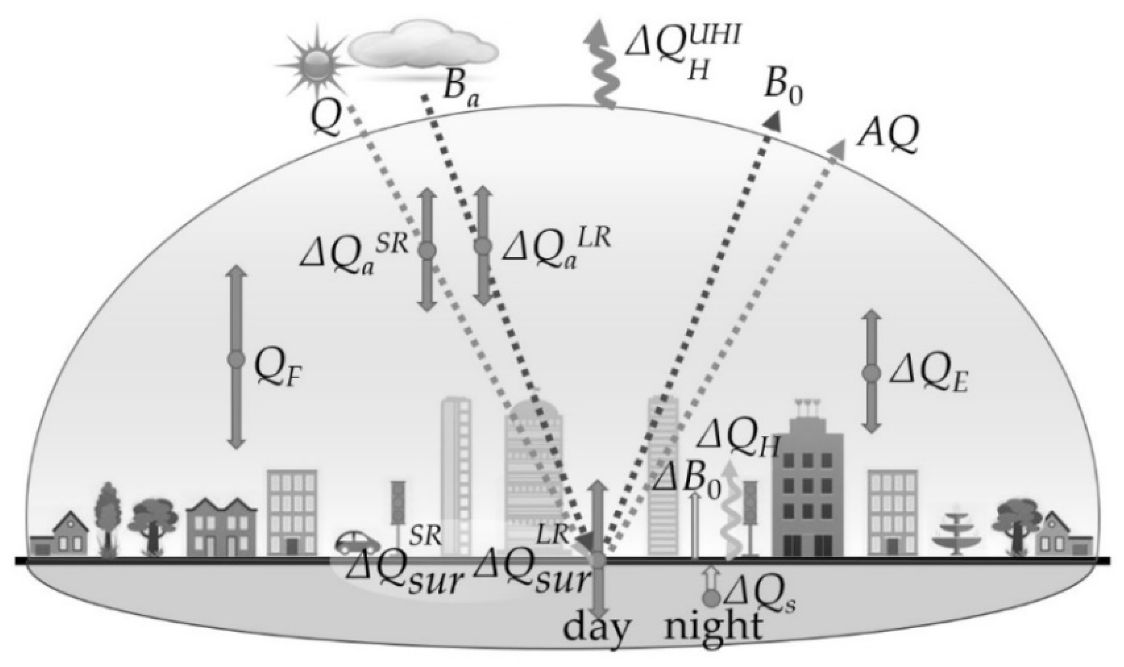
To construct the quantitative energy model, we assume that UHI covers a spatial region with changed, in comparison with the background, characteristics of reflection, absorption, and emission of energy that cause an increase in temperature. Within the framework of this model, the change in the absorption of energy from external sources and its emission into the outer space is estimated without a detailed analysis of the energy redistribution inside the UHI. Figure 1 illustrates schematically the main changes in the heat and radiation fluxes that cause the UHI formation.

The sun (radiation flux Q) and the atmosphere (radiation flux B_a) are the main external energy sources. The energy is accumulated in UHI, first, due to the difference in the reflective (and, accordingly, absorptive) properties of the urban surface as compared to the countryside (change in the flux Q_sur). The second factor is the extra absorption of both the shortwave and longwave radiation in the city by anthropogenic constituents, including water vapor (change in the flux Q_a). Third, one of the important causes for the UHI formation is the absence of energy consumption for evaporation, since it was found that in the countryside the hidden heat flux for water evaporation Q_E is much larger. Finally, direct heat emissions from the combustion of all types of fuel and the consumption of electricity are considered as the main reason for the UHI formation. This internal energy source is referred to as the anthropogenic heat flux Q_F.

It is obvious that as the air temperature in UHI increases, the value of the turbulent heat flux Q_H, which serves as an evacuator of excess energy, should increase too.

Thus, in the general form, the equation for the radiation flux Q_UHI providing for a temperature increase in UHI can be written as

Q_UHI = Q_F + ΔQ_sur + ΔQ_a + ΔQ_E − ΔQ_H^UHI

(1)

where Q_F is the anthropogenic heat flux in the city, ΔQ_sur = ΔQ_sur^SR + ΔQ_sur^LR is the difference between shortwave (ΔQ_sur^SR = Q_urb.sur^SR − Q_rur.sur^SR) and longwave (ΔQ_sur^LR = Q_urb.sur^LR − Q_rur.sur^LR) radiation fluxes absorbed by the urban (Q_urb.sur) and rural (Q_rur.sur) underlying surface, ΔQ_a = ΔQ_a^SR + ΔQ_a^LR is the difference of shortwave (ΔQ_a^SR = Q_urb.a^SR − Q_rur.a^SR) and longwave (ΔQ_a^LR = Q_urb.a^LR − Q_rur.a^LR) radiation fluxes absorbed by the urban and rural atmosphere, ΔQ_E is the difference in the urban and rural heat consumption for evaporation, and ΔQ_H^UHI = Q_H^urb − Q_H^rur is the difference in the urban and rural turbulent heat fluxes.

It should be also noted that the radiation flux ΔQ_sur associated with the changed absorption capacity of the urban surface is redistributed as follows: During the day, a part of the absorbed energy is spent directly in the increase in the UHI temperature (through an increase in the fluxes Q_H and B₀), while another part is accumulated in the deeper layers (road surface and building walls) due to the heat flux Q_S. At night, the accumulated energy is directed in the opposite direction from the deeper layers to the surface and spent in the increase in the UHI temperature. This fact should be taken into account when assessing the diurnal variation of the UHII.

2.1. Absorption of the Shortwave and Longwave Radiation by the Underlying Surface

The contribution of absorption of shortwave (SR) and longwave (LR) radiation to the formation of the UHI in the city can be determined from estimates of the following parameters:

ΔQ_sur^SR = Q_urb.sur^SR − Q_rur.sur^SR

(2)

ΔQ_sur^LR = Q_urb.sur^LR − Q_rur.sur^LR

(3)

where Q_urb.sur and Q_rur.sur are the radiation fluxes absorbed by the urban and rural underlying surfaces, respectively.

2.1.1. Absorption of Shortwave Radiation (ΔQ_sur^SR)

As was noted above, the decreased value of the reflection coefficient of urban surfaces in comparison with natural ones when exposed to the solar radiation in the daytime is the reason for their stronger heating [25,26] and, accordingly, an increase in their own radiation B₀, turbulent heat flux Q_H, and the heat flux to the deeper layers Q_S. It is obvious that the positive difference in the heat fluxes (B_0urb + Q_Hurb) − (B_0rur + Q_Hrur) in the daytime is the direct reason for the increased air temperature in the city (contributes to the UHI formation). At night, the UHI formation is affected by the daytime increase in Q_Surb in comparison with Q_Srur. Massive buildings and asphalted surfaces in the city in the daytime act as a storage for the energy of thermal radiation carried by an increased (compared to the rural value) flux Q_S. Obviously, to determine the effect of absorption of shortwave solar radiation on the UHII at different times of day, it is necessary to study in detail the diurnal dynamics of the following components of the heat balance equation: B₀, Q_H, and Q_S. However, to find the average contribution of changes in the absorption of solar radiation by the urban surface, it is sufficient to use the average values of Q_sur^SR.

The difference between the solar radiation absorbed in the city and outside the city can be estimated from the known urban A_urb and rural A_rur albedos as follows:

ΔQ_sur^SR = Q(1 − A_urb) − Q(1 − A_rur) = Q(A_rur − A_urb)

(4)

where Q is the total solar radiation and A_urb and A_rur are the albedos of the underlying surface in the urban and rural areas, respectively.

2.1.2. Absorption of Longwave Radiation (ΔQ_sur^LR)

It is obvious that a change in the underlying surface in the city, along with a change in the absorption capacity of solar radiation, also changes the absorption capacity of thermal (longwave) radiation of the atmosphere B_a.

Using an approach similar to the calculation of the difference between the absorbed solar radiation in the city and in the countryside (Equation (4)), we can estimate the difference between the absorbed longwave radiation in the city and outside the city using the following equation:

ΔQ_sur^LR = B_a(1 − K_urb) − B_a(1 − K_rur) = B_a(K_rur − K_urb)

(5)

where K_urb and K_rur are the integral reflection coefficients for the longwave radiation in the urban and rural areas, respectively.

It should be noted that Equations (4) and (5) can be directly used to determine the diurnal average contribution of these components to an increase in the UHII. However, as was already mentioned, the process of redistribution of the energy absorbed by the urban surface is inertial. Therefore, we propose the use of the following equations to estimate the diurnal variation of the contribution of these components:

$$\mathsf{\Delta }{Q}_{sur}{}^{SR}=\frac{1}{\tau }{{\displaystyle \int }}_{-\tau }^{0}Q\left(t\right)(A_{rur}-A_{urb})dt$$

(6)

$$\mathsf{\Delta }{Q}_{sur}{}^{LR}=\frac{1}{\tau }{{\displaystyle \int }}_{-\tau }^{0}Ba\left(t\right)(K_{rur}-K_{urb})dt$$

(7)

where τ is some time interval preceding the time of determination of the UHII t = 0.

2.2. Estimation of Atmospheric Absorption of the Shortwave and Longwave Radiation

The change in the fluxes of shortwave and longwave radiation in the atmosphere due to the absorption by anthropogenic atmospheric constituents can be determined as

ΔQ_a^SR = ΔQ_W^SR + ΔQ_p^SR

(8)

ΔQ_a^LR = ΔQ_W^LR + ΔQ_p^LR

(9)

where ΔQ_W is the change in the radiation fluxes due to absorption by water vapor and ΔQ_p is the change in the radiation fluxes due to absorption by minor gas constituents and aerosol of anthropogenic origin.

2.2.1. Absorption of Shortwave Radiation by Urban Water Vapor (ΔQ_W^SR)

The change in the flux of solar radiation due to absorption by urban water vapor can be most easily estimated from direct measurements of humidity in the city W_urb and in the rural area W_rur [24] using the results of simulation of solar radiation fluxes Q for different humidity [27]. If we know the values of shortwave solar radiation fluxes incident on the Earth’s surface in the spectral range 0.2–5.0 μm for winter and summer meteorological conditions with characteristic minimum, average, and maximum values of the total water vapor content, then we can calculate the increment of the solar radiation flux 𝜕Q at a change in the total water vapor content by 𝜕W in the entire range of possible atmospheric conditions.

Then, from the measured solar radiation flux Q and the estimated difference between the urban and rural total water vapor content ΔW = W_urb − W_rur, we can determine the difference ΔQ_W^SR = Q_urb − Q_rur using the following equation:

$$\mathsf{\Delta }{Q}_W{}^{SR}=-Q\frac{\partial Q/\partial W}{Q}\Delta W$$

(10)

where the normalized derivative $\frac{\partial Q/\partial W}{Q}$ determined from the simulated solar radiation fluxes for various humidity [27] characterizes the relative change of the solar radiation flux Q at a change in the total water vapor content W in the atmosphere.

2.2.2. Absorption of Longwave Radiation by Urban Water Vapor (ΔQ_W^LR)

The change in the longwave radiation flux B_a due to anthropogenic water vapor in the urban atmosphere, as in the case of shortwave radiation, can be estimated from downward longwave fluxes simulated for winter and summer conditions at different total water vapor values [28]. The values of downward fluxes of longwave radiation in the spectral range 0–3000 cm⁻¹ (wavelengths longer than 3.3 μm) for winter and summer meteorological conditions at characteristic minimum, average, and maximum values of the total water vapor content are given in [28]. These results allow us to calculate the increment of the longwave radiation flux 𝜕B_a as the total water vapor content changes by 𝜕W, which is needed for determination of the normalized derivative $\frac{\partial Ba/\partial W}{Ba}$. The parameter $\frac{\partial Ba/\partial W}{Ba}$ characterizes the relative change of the longwave radiation flux B_a at the change of the total water vapor content in the atmosphere W.

Then, using the measured longwave radiation flux B_a and the difference between the urban and rural total water vapor contents ΔW = W_urb − W_rur estimated from measurements of the meteorological parameters with the mobile station at the territory of the city and its suburbs, we can determine the difference ΔQ_W^LR = −ΔB_a − ΔQ_W^SR, where ΔB_a = B_{a urb}− B_{a rur}, which is the reason for an increase in temperature in the city:

$$\mathsf{\Delta }{Q}_W{}^{LR}=B_a\frac{\delta B_a/\delta W}{B_a}\mathsf{\Delta }W-\mathsf{\Delta }{Q}_W{}^{SR}$$

(11)

The subtraction of ΔQ_W^SR in Equation (11) is explained by the fact that the thermal radiation of the atmosphere within UHI increases due to absorption of not only the longwave but also solar radiation by water vapor.

2.2.3. Absorption by Minor Gas Constituents and Aerosol of Anthropogenic Origin (ΔQ_p^SR and ΔQ_p^LR)

The studies of pollution in a city with a moderate pollution level [29,30,31,32,33] have shown that the mass content of all pollutants is several orders of magnitude lower than the difference in the mass water vapor content in the city and outside the city. In this connection, without making an accurate estimation of changes in the fluxes of shortwave and longwave radiation due to absorption by minor gas constituents and aerosol of anthropogenic origin ΔQ_p^SR and ΔQ_p^LR, we can assert that ΔQ_p^SR and ΔQ_p^LR are much smaller than ΔQ_W^SR and ΔQ_W^LR. Therefore, they can be neglected when determining the reasons for the UHI formation. Then, we obtain that

ΔQ_a^SR ≈ ΔQ_W^SR

ΔQ_a^LR ≈ ΔQ_W^LR

and, consequently, the change in the absorptivity of the urban atmosphere has a little effect on the UHI formation.

2.3. Estimation of the Effect of Lower Energy Consumption for Water Evaporation in the City (ΔQ_E) on Formation of the Urban Heat Island

One of the most significant factors forming the urban heat island, according to many authors, is the decreased energy consumed for evaporation of water in the city as compared to the background area [11].

The effect of lower energy consumption for water evaporation in the city on the UHI formation in Tomsk was estimated from calculation of the heat flux associated with evaporation and condensation of water vapor [23] and measurements of the absolute humidity in the city and in the background region [24]. The value of ΔQ_E was calculated as follows:

ΔQ_E ≈ Q_E(a_rur − a_urb)/a_rur

(12)

where Q_E is the heat flux associated with evaporation and condensation of water vapor and a_urb and a_rur are the urban and rural absolute humidity values in g/m³.

2.4. Anthropogenic Heat Flux

Obviously, within the framework of a human life, almost all energy consumed by a person is sooner or later transformed into heat, which is the reason for the increase in the UHII. In this connection, neglecting the outflow of an insignificant amount of energy from UHI due to street lighting and other sources, the anthropogenic heat flux can be estimated as follows:

Q_F = Q_FF + Q_FE

(13)

where Q_FF is the anthropogenic heat from burnt fuel (enterprises, vehicles, and utility gas) and Q_FE is the heat from consumed electric energy. To determine these components, we can request the statistical data on the consumed electric energy and fuel per month in the relevant services and then calculate the average heat flux, taking into account the specific heat of combustion of different types of fuel. If it is necessary to determine more accurately the contribution of each component, we have to analyze all the main ways of transformation of electric energy and energy from fuel combustion to determine the redistribution of energy consumption within the standard working week and time of day and to estimate the fraction of energy leaving the city.

2.5. Turbulent Heat Flux

It is obvious that the outflow of the accumulated heat from UHI is mainly determined by the difference in turbulent fluxes in the city and outside the city ΔQ_H^UHI = Q_H^urb − Q_H^rur. Using the gradient method for determining the turbulent heat flux [23], we can write the following equation for Q_H:

$$Q_H={kC}_p\rho \frac{\partial \mathrm{T}}{\partial \mathrm{h}}$$

(14)

where k is the turbulence coefficient (m²/s), 𝜕T/𝜕h is the vertical temperature gradient (°C/m), C_p = 1006 J/(kg °C), and ρ is the air density (1.25 kg/m³).

2.6. Calculation of the UHII

If for the vertical temperature gradient we use the temperature difference 𝜕T = T_h2 − T_h1 with the height increment 𝜕h = h₂ − h₁ equal to the UHI height 𝜕h = $h_{UHI}$, then assuming that the urban and rural air temperatures above h_UHI coincide, i.e., T_h2^urb = T_h2^rur, we obtain the following equation for the difference between the urban and rural turbulent heat fluxes:

$$\mathsf{\Delta }=Q_H{}^{UHI}{kC}_p\rho \frac{\mathsf{\Delta }{T}_{UHI}}{h_{UHI}}$$

(15)

where $\mathsf{\Delta }{T}_{UHI}$= T_h1^urb − T_h1^rur is the increment of the near-surface temperature in the city due to anthropogenic changes (UHII), in °C, and h_UHI is the UHI height, in m.

Then, we can use the Matveev equation [34,35] proposed for estimation of the contribution of the anthropogenic heat flux to an increase in the UHII:

$$\mathsf{\Delta }{T}_{UHI}=\frac{Q_{F}l}{C_p\rho h_{UHI}V}$$

(16)

where Q_F is the anthropogenic heat flux, in W/m²; V is the wind speed, in m/s; and l is the linear size of the city in the wind direction, in m. The physical meaning of this equation is the following: if the air column moves within the city during the time t = l/V and the heat entering it spreads to the height h, then its temperature increases by ∆T.

In our case, the anthropogenic heat flux in Equation (16) should obviously be replaced with the sum of all heat fluxes causing the UHI formation:

Q_UHI = ΔQ_sur + ΔQ_a + ΔQ_E + Q_F − ΔQ_H^UHI = Q₊ − ΔQ_H^UHI

(17)

Thus, Equation (16) for estimating the contributions of all the heat fluxes given by Equation (17) to the increase in the UHII with allowance for the turbulent heat flux given by Equations (14) and (15) has the following form:

$$\mathsf{\Delta }{T}_{UHI}=\frac{\left(Q_{+}-k{C}_p\rho \frac{\mathsf{\Delta }{T}_{UHI}}{h_{UHI}}\right)l}{C_p\rho h_{UHI}V}$$

(18)

Then, solving the obtained equation for $\mathsf{\Delta }{T}_{UHI}$, we obtain the following equation for the UHII:

$$\mathsf{\Delta }{T}_{UHI}\frac{l{Q}_{+}}{C_p\rho h_{UHI}\left(V+V_H\right)}$$

(19)

where $V_H=\frac{kl}{h_{UHI}^2}$ has the meaning of the rate of turbulent heat outflow outside the UHI limits, in m/s, and V is the speed of horizontal UHI motion, in m/s.

It should be noted here that the resulting equation is similar to the Matveev Equation (16) with the only difference that the numerator includes the sum of all the heat fluxes characterizing the energy inflow to the UHI region and the wind speed in the denominator is replaced with the sum of the wind speed and some parameter $V_H$, which has the meaning of the speed of turbulent heat outflow from UHI. In this case, the speed V is determined by the speed of wind-driven drift of the “city cap”. In the case of a constant wind direction, the drift speed is determined by the absolute value of the wind speed. In situations that the wind direction changes faster than the time needed for the “city cap” to be completely displaced by the wind V = V_drift:

$$V_{drift}=|<V{>}_t|=<\{V_x{V}_y\}{>}_t=\sqrt{{\left(\frac{1}{t}{{\displaystyle \int }}_{-t}^0{V}_x\left(t^{\prime }\right)d{t}^{\prime }\right)}^2+{\left(\frac{1}{t}{{\displaystyle \int }}_{-t}^0{V}_y\left(t^{\prime }\right)d{t}^{\prime }\right)}^2}$$

(20)

where t is the time interval for averaging; it should be t > l/V.

Thus, the presented equations allow us to estimate the heat fluxes characterizing the heat inflow to the UHI region, while Equation (19) allows estimation of the UHII in the form of the temperature increment. We call this model an energy model because it does not allow us to analyze the heterogeneity of the air temperature distribution in the city depending on the building density, location of large enterprises, and other factors. In addition, based on this model, it is impossible to analyze the smooth decrease in the UHII with height. This model corresponds to the moderate increase in the air temperature within the volume V_UHI = S_UHI × h_UHI. However, the results of testing this model have shown that, with the correct choice of the parameter h_UHI, the calculated UHII is in good agreement with direct measurements.

3. Testing of the Model against Direct Measurements of Heat Island in Tomsk as an Example

3.1. Experimental Site, Measurement Systems, and Statistical Information

To test the proposed model, a series of experiments on direct UHI measurements was conducted. The urban heat island and humidity were studied in the territory of Tomsk, which had the total area of 294.6 km² and population of 528,600 people (for 2009) [24]. The meteorological parameters were measured in the period of 2004–2010 with the AKV-2 mobile station [29] on the chassis of a GAZ-66 boxcar. The mobile station was made by the V.E. Zuev Institute of Atmospheric Optics SB RAS in 2004. The station equipment allowed automatic every-second measurements of air temperature and humidity; wind speed and direction; total solar radiation; size spectrum of aerosol; and concentrations of gases NO, NO₂, O₃, SO₂, CO, and CO₂.

The route for the mobile station was chosen to provide for the maximal coverage of all the main highways of the city for the minimal time [32]. It took several hours for the mobile station to complete the given route. For this time, the values of air temperature and humidity varied (natural daily variation), which could significantly distort the UHI size and intensity determined from the difference between urban and rural values of meteorological parameters. In this connection, a correction for the natural daily variation was introduced.

The background values of air temperature and humidity for different wind directions were taken from two sites: the TOR station and the meteorological station located in the eastern and southern suburbs of Tomsk, respectively. Since the meteorological parameters were measured every hour at the TOR station and every three hours at the meteorological station, the TOR station was taken as the main background site. Measurements at the meteorological station were used only in the westerly wind when the TOR station was influenced by the air flow that passed through the city.

Table 1. Data needed to calculate the components of additional heat influx temperature increment in the city, measurement systems, and measurement periods.

Data Needed for Calculation	Measurement Systems, Statistical Databases	Measurement Period, Its Characteristics	Ref.
Q—total solar radiation, W/m2 t—air temperature, °C Rh—air humidity, % v—wind speed, m/s P—pressure, Pa	TOR station	Every-minute (with hourly averaging) continuous measurements of background values of meteorological parameters at a stationary observation site on the eastern side of the city	[36,37]
t—air temperature, °C Rh—air humidity, % v—wind speed, m/s P—pressure, Pa	Tomsk Center for Hydrometeorology and Environmental Monitoring—branch of the West-Siberian Hydrometeorology and Environmental Monitoring	Continuous (every 3 h) measurements of background values of meteorological parameters at a stationary observation site on the southern side of the city	[38]
t—air temperature, °C Rh—air humidity, % v—wind speed, m/s P—pressure, Pa	AKV-2 mobile station	Every-second (with minute averaging) measurements of urban and background meteorological parameters at the mobile station with reference to coordinates. Twelve S-route trips around the city and the background area.	[29,30,31,32,33]
*Q↑—solar radiation flux reflected by the surface, W/m2 *Q↓—solar radiation flux incident on the surface, W/m2	Optik-E AN-30 flying laboratory	Every-second (with minute averaging) measurements of solar radiation fluxes from aircraft with reference to coordinates. One flight in a month over the city and the background area.	[39,40]
t—air temperature, °C Rh—air humidity, % v—wind speed, m/s P—pressure, Pa	BEC observatory	Every-minute (with hourly averaging) measurements of background values of meteorological parameters at a stationary observation site on the eastern side of the city at heights of 10, 20, 30, 40 m	[41]
Amount of fuel (tons) consumed by large and small enterprises and vehicles	Tomskstat	Annual statistical data	[42]
Amount of generated electrical energy (kW h) and heat energy (Gcal) for heating of buildings	Territorial Generating Company No. 11, Tomsk branch	Monthly statistical data	[43]
Amount of consumed electrical energy (kW h)	Tomskenergosbyt regional energy retail company	Monthly statistical data	[44]

*A = Q↑/Q↓, A—albedo of the underlying surface

presents the data needed to calculate the components of additional heat influx and temperature increment in the city and characterizes the measurement systems and periods.

3.2. Estimation of Heat Fluxes from Measurements of Meteorological Parameters

3.2.1. Estimation of Absorption of Shortwave and Longwave Radiation by the Underlying Surface

The presence of a large number of massive buildings and asphalted surfaces in the city significantly affects the thermodynamic conditions. To assess the possibility of heat accumulation by the urban underlying surface during the day and subsequent heat release at night, we first determined the mass of building materials absorbing radiation, namely building walls and asphalt. When analyzing the development of Tomsk [45], it was found that about 20% of the UHI area (S_UHI = 50 km²) is occupied by houses with an average height of 15 m, 50% is asphalted, and 30% is parks and plantings. The area of house walls within UHI is about 17 km². With an average wall thickness of 0.5 m and an average density of 2000 kg/m³, this amounts to 17 × 10⁹ kg. With an average asphalt concrete thickness of 30 cm and a density of 2300 kg/m³, its mass within UHI is also about 17 × 10⁹ kg.

Then, with the average heat capacity of building materials (brickwork, concrete, asphalt concrete, etc.) C_p = 0.9 J/(kg K), an increase in the temperature of asphalt concrete and outer walls of houses by only 1 °C allows accumulation of about 3 × 10¹⁰ J of thermal energy. Accumulation of this amount of energy due to absorption of radiation in a built-up area within UHI (S = 35 km²) in the daytime (for 12 h) provides the radiation flux of 20 W/m².

Thus, we can conclude that the change in characteristics of the underlying surface in the city allows absorption and subsequent emission of radiation fluxes exceeding the background (suburban) values by tens or even hundreds of watts per square meter.

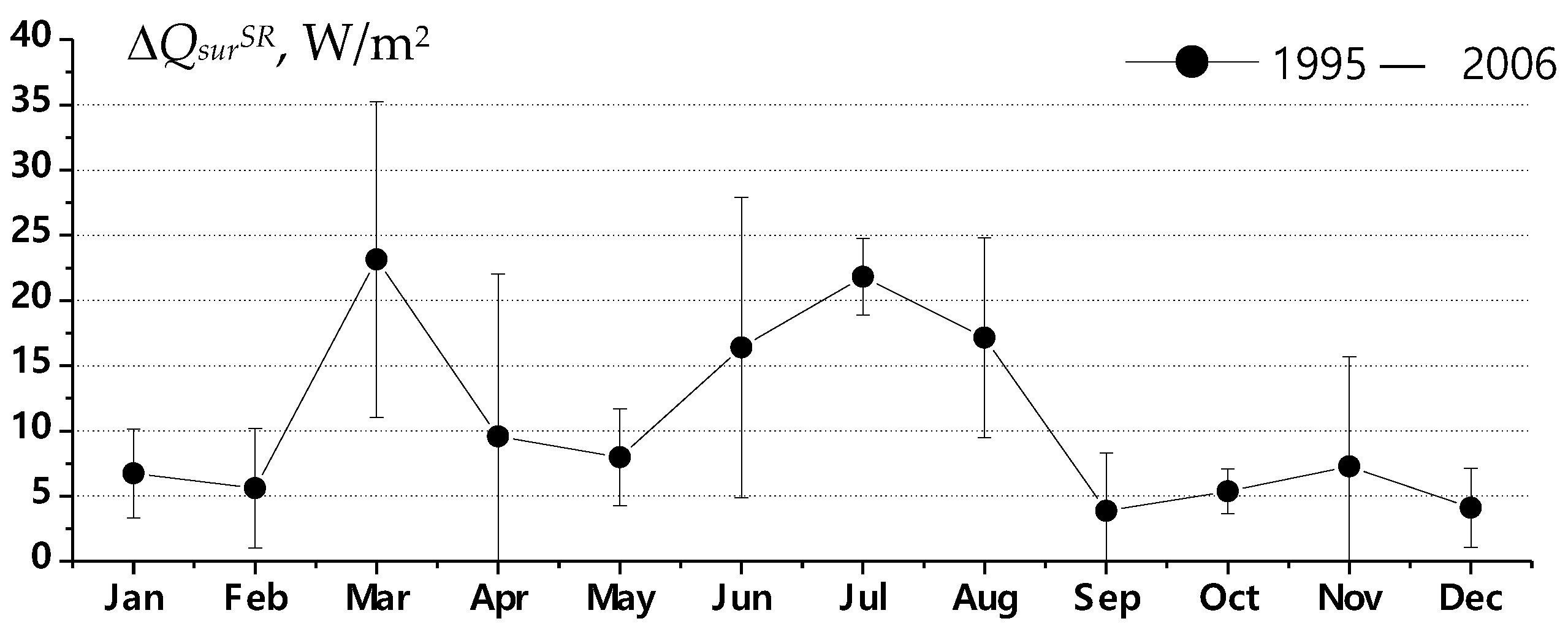
Figure 2 shows the annual profile of ΔQ_sur^SR calculated by Equation (6) upon averaging for the period of 1995–2005.

One can see that the diurnal average value of ΔQ_sur^SR is about 5 W/m² in winter and fall and 15–20 W/m² in summer. The marked increase in ΔQ_sur^SR in March as compared to the winter months can be explained by the marked difference in the urban A_urb and rural A_rur albedos in this period [40]. In March, the snow in the city had almost melted, while outside the city there was a stable snow cover.

3.2.2. Absorption of Longwave Radiation (ΔQ_sur^LR)

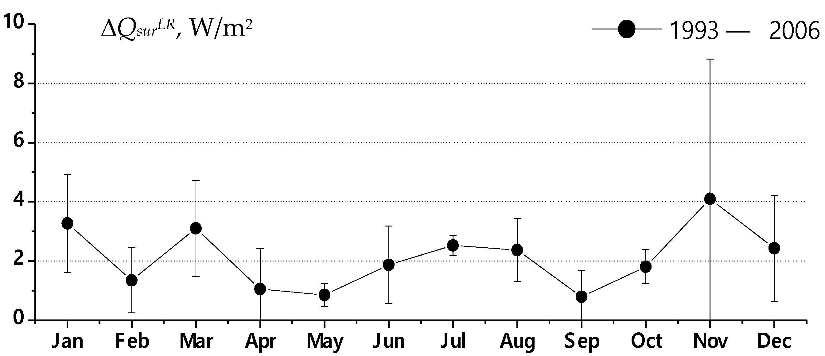
The analysis of spectral dependences of the reflection coefficients of building materials [46] and various types of the underlying surface [47] has shown that the integral reflection coefficient of the underlying surface of different types and various building materials in the longwave range (longer than 3 μm) is an order of magnitude smaller than the reflection coefficient in the shortwave range (from 0.4 to 3 μm). Figure 3 shows the annual profile of ΔQ_sur^LR averaged for the period of 1995–2005. It can be seen that the diurnal average value of ΔQ_sur^LR is smaller than 5 W/m².

3.2.3. Estimation of Atmospheric Absorption of Shortwave and Longwave Radiation

The results of the simulation of solar radiation fluxes [27] yield the following values of the derivative 𝜕Q/𝜕W normalized to the value of the radiation flux Q (

Table 2. Relative change of the flux Q due to the change in W.

	Winter			Summer
	Min	Average	Max	Min	Average	Max
W, g/cm2	0.1	0.25	0.4	1.0	2.0	3.1
$\frac{\delta Q/\delta W}{Q}$$,\frac{1}{\mathrm{g}/{\mathrm{cm}}^2}$	−0.155	−0.127	−0.096	−0.033	−0.028	−0.023

). In our calculations, we used “winter” data for air temperature below 0 °C and “summer” data for positive air temperatures.

From these results, we can find, for example, that in winter, with an average rural value of the total water vapor content of 0.25 g/cm², if the urban value of the total water vapor content exceeds the rural one by 0.1 g/cm², the urban solar radiation flux coming to the Earth’s surface is 1.27% smaller than the rural one.

The increase in the total water vapor content in the city ΔW can be estimated from measurements of the absolute air humidity in the city and its environs [24]. Assuming that the excess of the absolute humidity in the city Δa extends to the height of the surface layer h_bound, which averages 300 m, we can determine ΔW = Δa h_bound. The results of the calculation of ΔW and ΔQ_W^SR are given in

Table 3. Estimates of ΔQ_W^SR from measurements of the mobile station.

Date, Local Time	Δa, g/m3	ΔWmob, g/cm2	Q, W/m2	ΔQWSR, W/m2
23 June 2004 11:00–12:00	−0.4	−0.012	317	−0.13
11 July 2005 14:30–17:30	0	0	240	0.00
26 August 2005 08:30–12:05	0.6	0.018	177	0.11
14 May 2009 15:00–17:30	0.6	0.018	361	0.21
31 May 2009 11:20–17:00	0.3	0.009	330	0.10
17 July 2009 02:00–07:00	0.4	0.012	337	0.13
25 December 2009 13:30–19:00	0.1	0.003	18	0.01
26 January 2010 13:00–17:00	0.06	0.0018	68	0.02
4 February 2010 00:00–03:40	0.07	0.0021	87	0.03
11 February 2010 12:20–16:20	0.06	0.0018	100	0.03
12 February 2010 20:00–23:00	0.04	0.0012	113	0.02
9 April 2010 11:30–16:20	0.03	0.009	216	0.06

.

One can see that the change in the solar radiation flux due to the additional absorption by water vapor in the city is tenths of a watt per square meter.

It should be emphasized that the solar radiation fluxes calculated for the same water vapor content should differ for the cases when water vapor is distributed vertically in accord with the meteorological models used in [27] and when its concentration in the surface layer of urban air is increased. However, since this difference, obviously, does not exceed 10–15%, the influence of anthropogenic moisture concentrated in the surface layer on the change in the solar radiation fluxes in our case can be estimated only from the change in the total content of water vapor.

The results of the simulation of solar radiation fluxes [28] give the following values of the derivative $\partial Ba/\partial W$ normalized to the value of the radiation flux B_a (see

Table 4. Relative change of the flux Ba due to the change in W.

	Winter			Summer
	Min	Average	Max	Min	Average	Max
W, g/cm2	0.1	0.25	0.4	1.0	2.0	3.1
$\frac{\delta B_a/\delta W}{B_a}$$,\frac{1}{\mathrm{g}/{\mathrm{cm}}^2}$	0.9	0.8	0.7	0.17	0.09	0.05

).

From these results, we can find, for example, that in the winter period, with an average rural value of the total water vapor content of 0.25 g/cm², if the urban value of the total water vapor content exceeds the rural one by 0.1 g/cm², the urban solar longwave radiation flux coming to the Earth’s surface is 8% smaller than the rural one.

The results of calculation of ΔQ_W^LR obtained similarly to ΔQ_W^SR are given in

Table 5. Estimates of ΔQ_W^LR from measurements of the mobile station.

Date, Time	Δa, g/m3	ΔW, g/cm2	Ba, W/m2	ΔQWLR, W/m2
23 June 2004 11:00–12:00	−0.4	−0.012	321	−0.52
11 July 2005 14:30–17:30	0	0	303	0.00
26 August 2005 08:30–12:05	0.6	0.018	296	0.90
14 May 2009 15:00–17:30	0.6	0.018	231	0.71
31 May 2009 11:20–17:00	0.3	0.009	309	0.47
17 July 2009 02:00–07:00	0.4	0.012	351	0.72
25 December 2009 13:30–19:00	0.1	0.003	110	0.30
26 January 2010 13:00–17:00	0.06	0.0018	121	0.20
4 February 2010 00:00–03:40	0.07	0.0021	122	0.23
11 February 2010 12:20–16:20	0.06	0.0018	123	0.20
12 February 2010 20:00–23:00	0.04	0.0012	120	0.13
9 April 2010 11:30–16:20	0.03	0.009	166	0.25

.

One can see that the change in the longwave solar radiation flux due to the additional absorption by water vapor in the city is tenths of a watt per square meter.

Thus, we can conclude that atmospheric water vapor in the city absorbs shortwave and longwave radiation, thereby increasing the flux B_a as compared to the rural area by the value ΔB_a = ΔQ_W^LR + ΔQ_W^SR, which is smaller than 0.3 W/m² in winter and about 1 W/m² in summer. The longwave solar radiation flux increases by ΔB_a due to absorption of the shortwave and longwave radiation to different degrees: in the summer period, ΔQ_W^LR exceeds ΔQ_W^SR by several times, while in the winter period ΔQ_W^LR exceeds ΔQ_W^SR by an order of magnitude.

3.2.4. Estimation of the Effect of Lower Energy Consumption for Water Evaporation in the City (ΔQ_E) on the UHI Formation

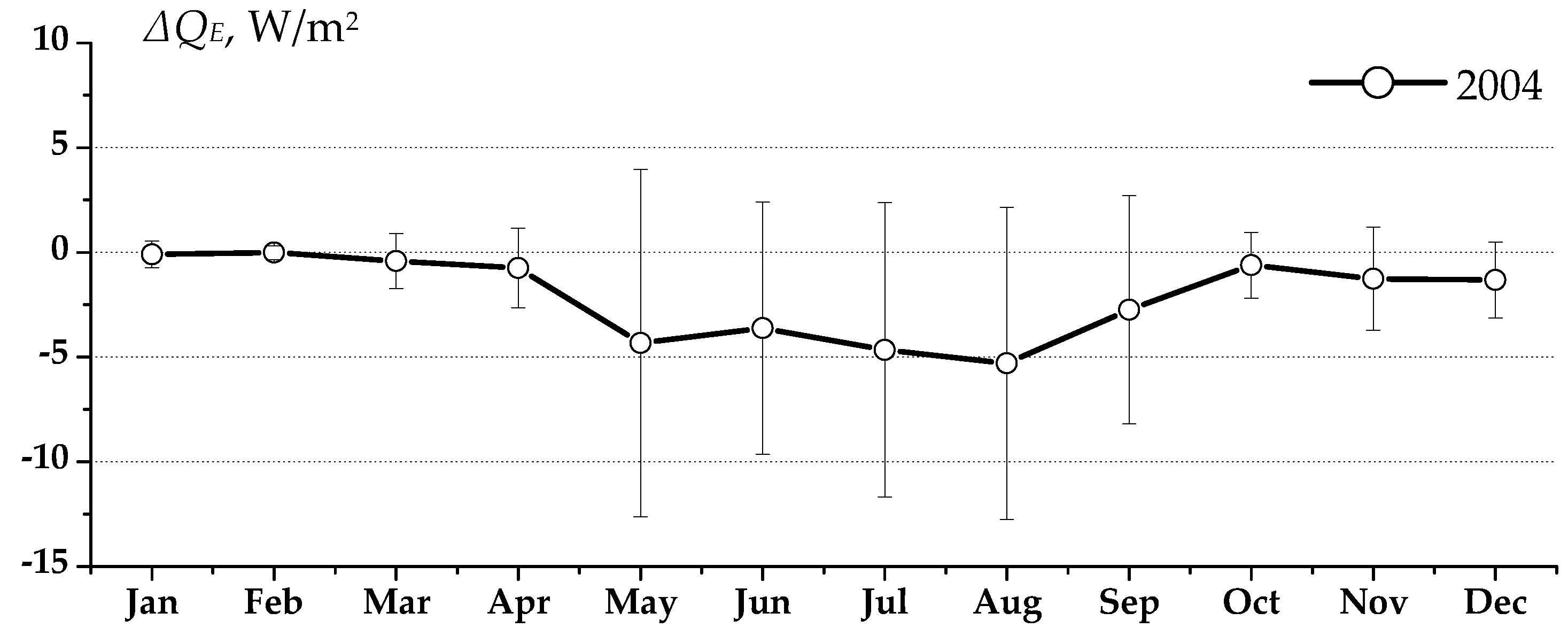
Figure 4 shows the results of the calculation of ΔQ_E for 2004.

Our estimates have shown that in winter there is no difference in consumption for water evaporation at all, since the measurements of the extra urban water vapor coincide with the estimate of the water vapor generated from the combustion of all types of fuel. In summer, the cost for water evaporation within UHI can reach minus 6 W/m².

Thus, we can conclude that this component is not decisive, as is often noted in the literature. On the contrary, it may act with the opposite sign, as in our case, i.e., reduce the UHII, although insignificantly.

3.2.5. Estimation of the Effect of Anthropogenic Heat Emissions on the UHI Formation

The map of the location of main industrial enterprises against the background of residential quarters of Tomsk is given in [48]. Based on measurements of the temperature distribution in the city, it was shown that the UHII in Tomsk [24] is in good agreement with the density of residential and industrial buildings, whose area is significantly smaller than the total area of Tomsk.

Earlier, we estimated the average value of the anthropogenic heat flux Q_F [49]. The calculations used data on the consumed fuel and electric energy for the entire city having an area of 294.6 km². It is obvious that the calculation of the contribution of anthropogenic heat flux to the UHI formation should be restricted to the data on fuel and electric energy consumption within the UHI area S_UHI, which in this case is about 50 km². The anthropogenic heat flux within the UHI area is denoted as Q_F^UHI.

Based on the information received from the Federal State Statistics Service [42], we can conclude that the UHI area S_UHI houses about 70% of the Tomsk population and about 70% of industrial enterprises. Thus, we can assume that about 70% of energy is spent within the area S_UHI = 50 km².

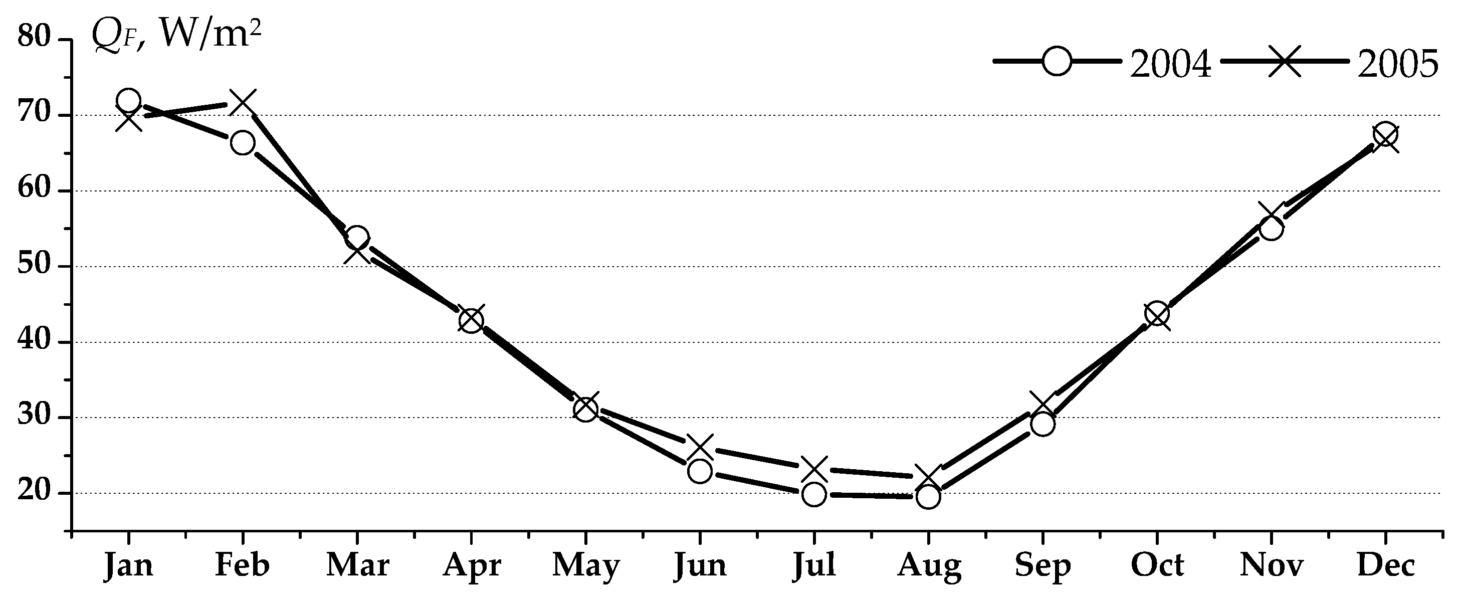
The distribution of the anthropogenic heat flux Q_F^UHI emitted within UHI as calculated with allowance for the UHI area S_UHI = 50 km² and the fraction of energy (70%) spent within this area, as well as the annual dynamics of energy consumption, is shown in Figure 5.

It can be seen from Figure 5 that the value of the anthropogenic heat flux within UHI Q_F^UHI reaches 70–75 W/m² in the winter months and 20–25 W/m² in the summer months, which is 4 to 5 times higher than the average urban values of Q_F.

3.3. Relation between the Factors of UHI Formation in Tomsk

It should be noted that Equation (19) proposed for calculating the UHII includes not only meteorological parameters measured with our equipment, but also the parameter h_UHI, which was not analyzed in this paper. However, the comparison of the UHII calculated by Equation (19) with direct measurements by the mobile station has shown that the parameter h_UHI for Tomsk can be taken constant and equal to 100 m. We can assume that for any chosen city this parameter will be constant as well.

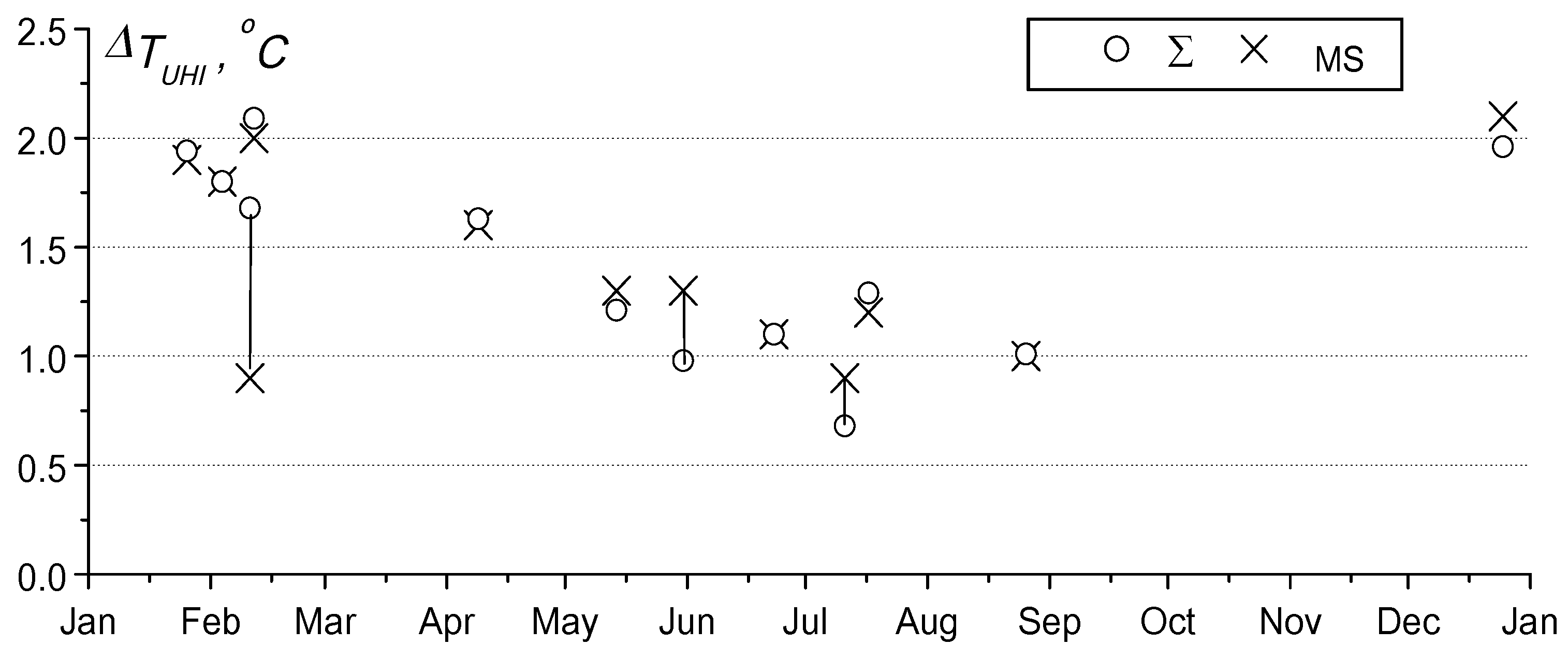
Figure 6 compares the UHII calculated by Equation (19) with direct measurements by the mobile station. In the period of 2004–2010, a total of 12 measurements with the mobile station were carried out [24]. For a more illustrative demonstration of the seasonal dependence of the UHII, the results are grouped for months, regardless of the year. A good agreement of the model results with direct measurements is observed in 11 cases. Unfortunately, we failed to explain the discrepancy observed on 11 February 2010, within the framework of the proposed approach. Nevertheless, it can be seen that the UHII is about 2 °C in winter and about 1 °C in summer.

Table 6. Calculated contributions of different factors to the UHI formation (°C) for the measurements of the mobile station.

Date, Local Time	Weather Conditions	ΔT								ΔTUHI
		QF	$\Delta {\mathit{Q}}_{\mathit{s}\mathit{u}\mathit{r}}^{\mathit{S}\mathit{R}}$	$\Delta {\mathit{Q}}_{\mathit{s}\mathit{u}\mathit{r}}^{\mathit{L}\mathit{R}}$	$\Delta {\mathit{Q}}_{\mathit{a}}^{\mathit{S}\mathit{R}}$	$\Delta {\mathit{Q}}_{\mathit{a}}^{\mathit{L}\mathit{R}}$	∆QE	Q+	$\Delta {\mathit{Q}}_{\mathit{H}}^{\mathit{U}\mathit{H}\mathit{I}}$	*∑	*MS
23 June 2004 11:00–12:00	10/1 Cu Ci; NEE 2.1 m/s; No precipitation	1.34	0.51	0.13	0.00	0.00	0.16	2.14	−1.04	1.10	1.1
11 July 2005 14:30–17:30	7/4 Cu Ci; S 3 m/s; No precipitation	0.48	0.45	0.06	0.00	0.00	0.00	0.99	−0.31	0.68	0.9
26 August 2005 08:30–12:05	10/10 Ns; Calm; Light rain shower	3.59	0.00	0.43	0.02	0.15	−0.20	3.99	−2.98	1.01	1.0
14 May 2009 15:00–17:30	3/0 Ci fib; NWW 1.6 m/s; No precipitation	1.34	0.61	0.04	0.01	0.02	0.00	2.02	−0.81	1.21	1.3
31 May 2009 11:20–17:00	10/7 Cb Ci; SWW 1.6 m/s; Light rain shower	1.59	0.11	0.05	0.01	0.02	0.00	1.78	−0.80	0.98	1.3
17 July 2009 02:00–07:00	4/0 Ci; NEE 1.6 m/s; No precipitation	0.99	1.15	0.13	0.01	0.03	0.00	2.31	−1.02	1.29	1.2
25 December 2009 13:30–19:00	As Ci 10/0; S 2.4 m/s; Light snow	3.39	0.15	0.10	0.00	0.01	0.00	3.65	−1.69	1.96	2.1
26 January 2010 13:00–17:00	Clear sky; NNW 1.2 m/s; No precipitation; ice needles	3.84	1.13	0.13	0.00	0.01	0.00	5.11	−3.17	1.94	1.9
4 February 2010 00:00–03:40	Clear sky; NNE 2.1 m/s; No precipitation	2.79	0.38	0.04	0.00	0.01	0.00	3.22	−1.42	1.80	1.8
11 February 2010 12:20–16:20	Clear sky; NNE 1.7 m/s; No precipitation	2.48	0.17	0.04	0.00	0.01	0.00	2.70	−1.02	1.68	0.9
12 February 2010 20:00–23:00	Clear sky; S 1.7 m/s; No precipitation	3.81	1.03	0.06	0.00	0.01	0.00	4.91	−2.82	2.09	2.0
9 April 2010 11:30–16:20	Clear sky; W 1.6 m/s; No precipitation	2.84	0.30	0.06	0.00	0.01	0.00	3.21	−1.58	1.63	1.6

*Σ = Q+ + Q_H^UHI; MS is for the average UHII measured with the mobile station.

presents the calculated contributions of different factors to the formation of the heat island in Tomsk for the same 12 cases accompanied by the measurements at the mobile station.

Analyzing this table, we can see that if the turbulent heat outflow is not taken into account, then the Matveev equation gives strongly overestimated values. For example, for the case of 26 January 2010, we can see that, without the turbulent heat outflow, the calculated UHII is 2.5 higher than the actual value.

The comparison of the UHII calculated by the proposed approach with the measurements of the mobile station has demonstrated the good correlation of the results with the correlation coefficient of 0.82.

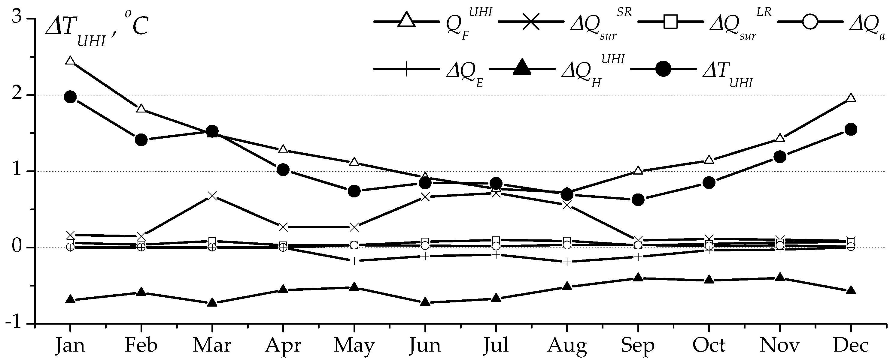
Figure 7 shows the monthly averaged UHII due to all the heat fluxes (19) in 2004.

It can be seen that the major energy contributor to Tomsk UHI is the anthropogenic heat flux: 80–90% of the total energy increment in winter and 40–50% in summer. The second most important contributor is the absorption of shortwave radiation by the urban underlying surface: 5–15% in winter and 40–50% in summer. The absorption of the longwave radiation by the urban underlying surface amounts to 2–5% in winter and summer, while the absorption by water vapor and atmospheric constituents is low—below 1%. Heat consumption for evaporation in winter is absent, and in summer it can slightly (up to 15%) reduce the UHII. The turbulent heat outflow significantly reduces the UHII: by 25–30% of the total heat influx in winter and 40–45% in summer.

4. Conclusions

Thus, the proposed equation for the calculation of UHII was obtained with allowance for the effect of all the main factors of UHI formation and their relative contributions in different seasons and times of day and under different atmospheric conditions. The model proposed in this study is based on the understanding and quantitative estimation of the physical causes of the difference between thermodynamic conditions of the city and countryside. Its main advantage is versatility. In this case, there is no need to calibrate the model for different climatic conditions of the geographic location of the analyzed city, since it does not matter which of the factors are of decisive importance. Moreover, in this model, heat fluxes affecting the UHI formation can be estimated with measurement facilities and statistical data different from those used by us. Thus, for example, to determine the albedo of the urban and rural underlying surface, we used the available data of the flying laboratory. Perhaps, these data can be obtained somewhat more readily with ground-based measurement facilities with fairly good averaging over the urban or rural area.

Testing the proposed model through comparison of the calculated UHII with the direct measurements by the mobile station in Tomsk has shown its good applicability for various observation conditions: seasons, time of day, and weather conditions.

The relative contributions of the main factors of UHI formation in Tomsk have been determined. The main contribution to the UHI formation is due to the anthropogenic heat emissions, followed by the absorption of shortwave radiation by the urban underlying surface. The absorption of longwave radiation by the urban underlying surface and the absorption by water vapor and atmospheric constituents are insignificant. Heat consumption for evaporation in winter is absent, and in summer it can slightly reduce the UHII.

Turbulent heat flux prevents a linear increase in the UHII with an increase in the sum of radiation fluxes providing the energy inflow to the UHI area. In the warm season, up to 50% of the absorbed energy is removed due to an increase in the turbulent heat flux in Tomsk.

It should be noted that the proposed model has one free parameter, namely the height of the heat island. Therefore, our following study will concentrate on the analysis of the factors determining this parameter. Tests of our model with the city of Tomsk taken as an example have shown that this parameter is fixed. Thus, the need to analyze UHI in significantly different climatic zones and for different kinds of cities encourages wide scientific cooperation.

References

- Landsberg, H.E. The Urban Climate; Academic Press: New York, NY, USA, 1981; p. 275. [Google Scholar]
- Belan, B.D. To the problem of contamination «top» formation over industrial centers. Atmos. Ocean. Opt. J. 1996, 9, 460–463. (In Russian) [Google Scholar]
- Stathopoulou, E.; Mihalakakou, G.; Santamouris, M.; Bagiorgas, H.S. On the impact of temperature on tropospheric ozone concentration levels in urban environments. J. Earth Syst. Sci. 2008, 117, 227–236. [Google Scholar] [CrossRef]
- Pantavou, A.; Theoharatos, G.; Mavrakis, A.; Santamouris, M. Evaluating thermal comfort conditions and health responses during an extremely hot summer in Athens. Build. Environ. 2011, 46, 339–344. [Google Scholar] [CrossRef]
- Santamouris, M.; Kolokotsa, D. On the impact of urban overheating and extreme climatic conditions on housing energy comfort and environmental quality of vulnerable population in Europe. Energy Build. 2015, 98, 125–133. [Google Scholar] [CrossRef]
- Sakka, A.; Santamouris, M.; Livada, I.; Nicol, F.; Wilson, M. On the thermal performance of low income housing during heat waves. Energy Build. 2012, 49, 69–77. [Google Scholar] [CrossRef]
- Oke, T.R. The energetic basis of the urban heat island. Q. J. R. Meteorol. Soc. 1982, 108, 1–24. [Google Scholar] [CrossRef]
- Oke, T.R.; Fuggle, R.F. Comparison of urban/rural counter and net radiation at night. Bound. Layer Meteorol. 1972, 2, 290–308. [Google Scholar] [CrossRef]
- Isakov, S.V.; Shklyaev, V.A. Determination of total impact of anthropogenic change surfaces, on the occurrence of the effect of “urban heat island” with the use of geographic information systems. Vestn. Orenbg. State Univ. 2014, 161, 178–182. [Google Scholar]
- Grimmond, C.S.B.; Oke, T.R. Comparison of heat fluxes from summertime observations in the suburbs of four North American cities. J. Appl. Meteorol. 1995, 34, 837–889. [Google Scholar] [CrossRef] [Green Version]
- Adebayo, Y.R. “Heat island” in a humid tropical city and its relationship with potential evaporation. Theor. Appl. Climatol. 1991, 43, 137–147. [Google Scholar] [CrossRef]
- Komarov, V.S.; Barinova, S.A.; Matveev, Y.L. Change of meteorological conditions in Siberian cities under the effect of anthropogenic factor. Atmos. Ocean. Opt. 2001, 14, 259–262. [Google Scholar]
- Belan, B.D.; Rasskazchikova, T.M. Impact of the urban area of Tomsk on the temperature-humidity regime of air. Atmos. Ocean. Opt. 2001, 14, 267–270. [Google Scholar]
- Oke, T.R. Boundary Layer Climates; Routledge: London, UK, 1987; p. 464. [Google Scholar]
- Unger, J. Intra-urban relationship between surface geometry and urban heat island: Review and new approach. Clim. Res. 2004, 27, 253–264. [Google Scholar] [CrossRef] [Green Version]
- Robbiati, F.O.; Cáceres, N.; Hick, E.C.; Suarez, M.; Soto, S.; Barea, G.; Matoff, E.; Galetto, L.; Imhof, L. Vegetative and thermal performance of an extensive vegetated roof located in the urban heat island of a semiarid region. Build. Environ. 2022, 212, 108791. [Google Scholar] [CrossRef]
- Stache, E.; Schilperoort, B.; Ottelé, M.; Jonkers, H.M. Comparative analysis in thermal behaviour of common urban building materials and vegetation and consequences for urban heat island effect. Build. Environ. 2021, in press. [Google Scholar] [CrossRef]
- Hoffmann, P.; Krueger, O.; Schlünzen, K.H. A statistical model for the urban heat island and its application to a climate change scenario. Int. J. Climatol. 2012, 32, 1238–1248. [Google Scholar] [CrossRef]
- Szymanowski, M.; Kryza, M. Local regression models for spatial interpolation of urban heat island—An example from Wrocław, SW Poland. Theor. Appl. Climatol. 2012, 108, 53–71. [Google Scholar] [CrossRef] [Green Version]
- Theeuwes, N.E.; Steeneveld, G.J.; Ronda, R.J.; Holtslag, A.A. A diagnostic equation for the daily maximum urban heat island effect for cities in northwestern Europe. Int. J. Climatol. 2017, 37, 443–454. [Google Scholar] [CrossRef]
- Sangiorgio, V.; Fiorito, F.; Santamouris, M. Development of a holistic urban heat island evaluation methodology. Sci. Rep. 2020, 10, 17913. [Google Scholar] [CrossRef]
- Dudorova, N.V.; Belan, B.D. Radiation balance of the underlying surface in Tomsk in 2004–2005. Opt. Atmos. I Okeana 2015, 28, 312–317. (In Russian) [Google Scholar] [CrossRef]
- Dudorova, N.V.; Belan, B.D. Thermal balance of the underlying surface in Tomsk in 2004–2005. Opt. Atmos. I Okeana 2015, 28, 229–237. (In Russian) [Google Scholar] [CrossRef]
- Dudorova, N.V.; Belan, B.D. Estimation of the intensity and size of the heat and moisture island in Tomsk from direct measurements. Opt. Atmos. I Okeana 2016, 29, 419–425. [Google Scholar] [CrossRef]
- Voogt, J.A.; Oke, T.R. Complete urban surface temperatures. J. Appl. Meteorol. 1997, 36, 1117–1132. [Google Scholar] [CrossRef]
- Voogt, J.A.; Oke, T.R. Effects of urban surface geometry on remotely-sensed surface temperature. Int. J. Remote Sens. 1998, 19, 895–920. [Google Scholar] [CrossRef]
- Chesnokova, T.Y.; Zhuravleva, T.B.; Ptashnik, I.V.; Chentsov, A.V. Simulation of solar radiative fluxes in the atmosphere using different models of water vapor continual absorption in typical condition of Western Siberia. Opt. Atmos. I Okeana 2013, 26, 100–107. (In Russian) [Google Scholar]
- Firsov, K.M.; Chesnokova, T.Y.; Bobrov, E.V. Role of water vapor continual absorption in the atmospheric longwave radiative processes of the surface layer in the Lower Volga region. Opt. Atmos. I Okeana 2014, 27, 665–672. (In Russian) [Google Scholar]
- Arshinov, M.Y.; Belan, B.D.; Davydov, D.K.; Ivlev, G.A.; Kozlov, A.V.; Pestunov, D.A.; Pokrovskii, E.V.; Simonenkov, D.V.; Uzhegova, N.V.; Fofonov, A.V. AKV-2 mobile station and its use in Tomsk city as an example. Atmos. Ocean. Opt. 2005, 18, 575–580. [Google Scholar]
- Belan, B.D.; Ivlev, G.A.; Pirogov, V.A.; Pokrovskij, E.V.; Simonenkov, D.V.; Uzhegova, N.V.; Fofonov, A.B. Comparative assessment of the air composition of industrial cities in Siberia during the cold period. Geogr. Nat. Resour. 2005. (In Russian) [Google Scholar] [CrossRef]
- Belan, B.D.; Ivlev, G.A.; Kozlov, A.S.; Marinaite, I.I.; Penenko, V.V.; Pokrovskii, E.V.; Simonenkov, D.V.; Fofonov, A.V.; Khodzher, T.V. Comparison of air composition over industrial cities of Siberia. Atmos. Ocean. Opt. 2007, 20, 387–396. [Google Scholar]
- Uzhegova, N.V.; Antokhin, P.N.; Belan, B.D.; Ivlev, G.A.; Kozlov, A.V.; Fofonov, A.V. Extraction of anthropogenic contribution to change of city’s air temperature, humidity, gas and aerosol composition. Opt. Atmos. I Okeana 2011, 24, 589–596. (In Russian) [Google Scholar]
- Uzhegova, N.V.; Antokhin, P.N.; Belan, B.D.; Ivlev, G.A.; Kozlov, A.V.; Fofonov, A.V. Daily variations of Tomsk air characteristics in cold season. Opt. Atmos. I Okeana 2011, 24, 782–789. (In Russian) [Google Scholar]
- Kondratiev, K.Y.; Matveev, L.T. The main factors in the formation of a heat island in a big city. Dokl. Earth Sci. 1999, 367, 253–256. (In Russian) [Google Scholar]
- Matveev, L.T.; Matveev, Y.L. Formation and features of a heat island in a big city. Dokl. Earth Sci. 2000, 370, 249–252. [Google Scholar]
- Davydov, D.K.; Belan, B.D.; Antokhin, P.N.; Antokhina, O.Y.; Antonovich, V.V.; Arshinova, V.G.; Arshinov, M.Y.; Akhlestin, A.Y.; Belan, S.B.; Dudorova, N.V.; et al. Monitoring of Atmospheric Parameters: 25 Years of the Tropospheric Ozone Research Station of the Institute of Atmospheric Optics, Siberian Branch, Russian Academy of Sciences. Atmos. Ocean. Opt. 2019, 32, 180–192. [Google Scholar] [CrossRef]
- Laboratory of Atmosphere Composition Climatology. Available online: https://lop.iao.ru/EN/ (accessed on 23 December 2021).
- Tomsk Center for Hydrometeorology and Environmental Monitoring. Available online: http://www.meteotomsk.ru/site/ (accessed on 23 December 2021).
- Arshinov, M.Y.; Belan, B.D.; Davydov, D.K.; Ivlev, G.A.; Kozlov, A.S.; Kozlov, V.S.; Panchenko, M.V.; Penner, I.E.; Pestunov, D.A.; Safatov, A.S.; et al. Aircraft laboratory Antonov-30 “Optik-E”: 20-year investigations of the environment. Opt. Atmos. I Okeana 2009, 22, 950–957. (In Russian) [Google Scholar]
- Belan, B.D.; Sklyadneva, T.K.; Uzhegova, N.V. The difference in the albedo of underlying surface in Novosibirsk and in the surroundings of Novosibirsk. Opt. Atmos. I Okeana 2005, 18, 238–241. (In Russian) [Google Scholar]
- Arshinov, M.Y.; Belan, B.D.; Davydov, D.K.; Ivlev, G.A.; Kozlov, A.V.; Pestunov, D.A.; Pokrovskii, E.V.; Tolmachev, G.N.; Fofonov, A.V. Sites for monitoring of greenhouse gases and gases oxidizing the atmosphere. Atmos. Ocean. Opt. 2007, 20, 45–53. [Google Scholar]
- Federal State Statistics Service. Available online: https://eng.rosstat.gov.ru/ (accessed on 23 December 2021).
- INTER RAO. TGK-11. Available online: http://tomsk.tgk11.com/english/ (accessed on 23 December 2021).
- Tomskenergosbyt. Available online: http://www.ensb.tomsk.ru/ (accessed on 23 December 2021).
- Google Earth. Available online: https://www.google.com/earth/ (accessed on 23 December 2021).
- Babichev, A.P.; Babushkina, N.A.; Bratkovskii, A.M. Physical Quantities: Directory; Grigoreva, I.S., Mejlikhova, E.Z., Eds.; Energoatomizdat: Moscow, Russia, 1991; p. 1231. [Google Scholar]
- Belward, A.; Loveland, T. The DIS 1 km Land Cover Data Set. IGBP Glob. Chang. Newsl. 1996, 27, 7–9. [Google Scholar]
- Yazikov, E.G.; Talovskaya, A.V.; Zhornyak, L.V. Assessment of the Ecological and Geochemical State of the Territory of Tomsk according to the Study of Dust Aerosols and Soils; TPU: Tomsk, Russia, 2010; p. 264. [Google Scholar]
- Belan, B.D.; Pelymskii, O.A.; Uzhegova, N.V. Study of the anthropogenic component of urban heat balance. Atmos. Ocean. Opt. 2009, 22, 441–445. [Google Scholar] [CrossRef]
Figure 1.
Main changes in the heat and radiation fluxes at the urban underlying surface that cause the formation of the urban heat island.
Figure 2.
Dynamics of the difference between the fluxes of absorbed shortwave radiation in the urban and rural areas ΔQsurSR.
Figure 3.
Dynamics of the difference between the fluxes of absorbed longwave radiation in the urban and rural areas.
Figure 4.
Dynamics of the difference in the heat fluxes associated with evaporation and condensation of water vapor in Tomsk and its background (rural) region.
Figure 5.
Annual dynamics of the anthropogenic heat flux QF emitted within the city in Tomsk.
Figure 6.
Comparison of the calculated temperature change in the city under the effect of all fluxes (∑) with that measured by the mobile station (MS).
Figure 7.
Air temperature increment in the city due to all the heat fluxes.