Article

Comparison between Air Temperature and Land Surface Temperature for the City of São Paulo, Brazil

by
Augusto Cezar Lima do Nascimento
1,*,
Emerson Galvani
2,
João Paulo Assis Gobo
3 and
Cássio Arthur Wollmann
4,*
1
Department of Earth Sciences, University of Bergen, Allégaten 41, 5007 Bergen, Norway
2
Department of Geography, University of São Paulo (USP), Professor Lineu Prestes Ave., Number 338, São Paulo 05508-900, Brazil
3
Department of Geography, Federal University of Rondônia (UNIR), Surubim Str., 4714-Lagoa, Porto Velho 76812-020, Brazil
4
Department of Geography, Federal University of Santa Maria (UFSM), Roraima Ave., Number 1000, Building 17, Room 1018, Camobi, Santa Maria 97105-900, Brazil
*
Authors to whom correspondence should be addressed.
Submission received: 31 December 2021 / Revised: 25 February 2022 / Accepted: 15 March 2022 / Published: 18 March 2022
(This article belongs to the Special Issue Advancement of Urban Heat Island Studies)

Abstract

:
This study aims to identify the relationship between changes in temperature regarding urbanization processes and seasonality in the city of São Paulo, located in the Tropic of Capricorn. The land surface temperature (LST) results were compared to official weather stations measurements, identifying in the spring–summer period 65.5% to 86.2% accuracy, while in the autumn–winter period, the results ranged from 58.6% to 93.1% accuracy, when considering the standard deviation and the temperature probe error. The mean MAE and mean RMSE range from 1.2 to 1.9 °C, with 83.0% of the values being ≤2.7 °C, and the coefficient of determination values are R = 0.81 in spring–summer and R = 0.82 in autumn–winter. Great thermal amplitude was estimated in the spring–summer season, with a difference in LST of the built-up space and rural area ranging from 5.8 and 11.5 °C, while in the autumn–winter season, the LST is more distributed through the city, with differences ranging from 4.4 to 8.5 °C. In addition, the current study suggests remote sensing as a reliable, cheap, and practical methodology to assist climate in order to support public policies and decision-making actions regarding environmental and urban planning.

1. Introduction

Cities are the most evident form of transformation of the natural landscape. The change in the elements of the climate has great ecological repercussions as it immediately affects the inhabitants through thermal discomfort and the concentration of pollutants [1,2,3,4,5].
Coverings of artificial surfaces, buildings, and human activities, concentrated in cities, significantly modify the radiation components of energy balance and wind near the surface, thus creating the cities’ unique climate [6,7,8,9,10]. In this sense, studies show that the increase in impermeable surfaces and large amounts of heat emissions, together with the low index of urban green areas, can cause excess heat storage, a reduction in the moisture content of the substrate, and, consequently, a reduction in latent heat fluxes and evapotranspiration processes, which are variables that can enhance the exposure to heat in the open air, thus favoring a feeling of thermal discomfort for human beings [11,12,13,14].
The absence or reduced network of weather stations, the low spatial coverage of equipment, the lack of articulation in between them, the errors in measurements passed by not-suitable installation methods, and the low availability of specialized professionals highlight remote sensing and geoprocessing techniques as decision-making tools to guide society and governments through risks associated to socio-environmental problems [15].
Interest in urban climate studies has increased not only because most of the Brazilian and world populations live in cities but also because of the degradation process of these environments and its effects on the quality of life of city dwellers [16]. The changes imposed on the components of the local climate system by the pattern of the country’s cities expose the population to the implications (thermal stress, compromised air quality, increased energy consumption, and the redefinition of urban planning) of urban heat islands (ICUs), which can be accentuated by global climate change [4,17].
The usage of the geographic information system has increased towards the urban climate study. Thus, evaluating the applicability of hardware [18,19], algorithms [20,21,22,23,24], and equations [25] is also a promising research field. Some studies have gone even further and applied a concise methodology and a well-constructed flowchart in a study case [26,27,28].
The correlation established between land surface temperature and air temperature assists us in understanding the processes related to a climate in each space and its urbanization [11,12,29,30]. Identifying the usability of remote sensing and spatial analyses techniques towards a scenario can contribute to climate monitoring once it allows the visualization of spatial distribution trends of climatological variables in areas without monitoring stations [25] in order to simulate processes and predict effects [31].
Climate monitoring is a strategy of paramount importance for managers and of great social impact since it is a way of identifying, predicting, and proposing solutions to the energy and supply crises that have plagued many nations historically; patterns and linearity can be found in the apparent climatic instability. In the Brazilian case, the difficulties go beyond the installation of meteorological stations to the lack of articulation between them since, in some Brazilian states, several private bodies and institutions collect data without a common information bank for access. Beyond that, there are ineffective collection data procedures and weather station maintenance in rural properties and areas since it is necessary to collect daily data from the devices if they are conventional. Lastly, the Brazilian government has found difficulties in acquiring automatic weather stations due to economics and the size of the country. The question of adapting the country to the climate certainly requires time, money, and material resources of great importance, which results in the urgency to carry out studies that may contribute to the administration’s decision-making processes and to guide society through the risks associated with socio-environmental problems.
Having historical and accurate climate monitoring helps to answer how the urbanization process and chaotic distribution of the demographic population generate impacts that have negative effects on climate change and generate climate changes that have negative effects on urban areas [32,33,34,35]. Thus, alternative methods to study climate changes, its causes, and its sites are of the most importance as the climate changes interfere with the life quality of the inhabitants of a city as it affects thermal comfort, whether negatively when generating heat islands or positively when generating freshness and cold islands. Finally, this study is concerned with identifying the relationship between surface temperature changes in urbanization processes and seasonality in the city of São Paulo, Brazil.

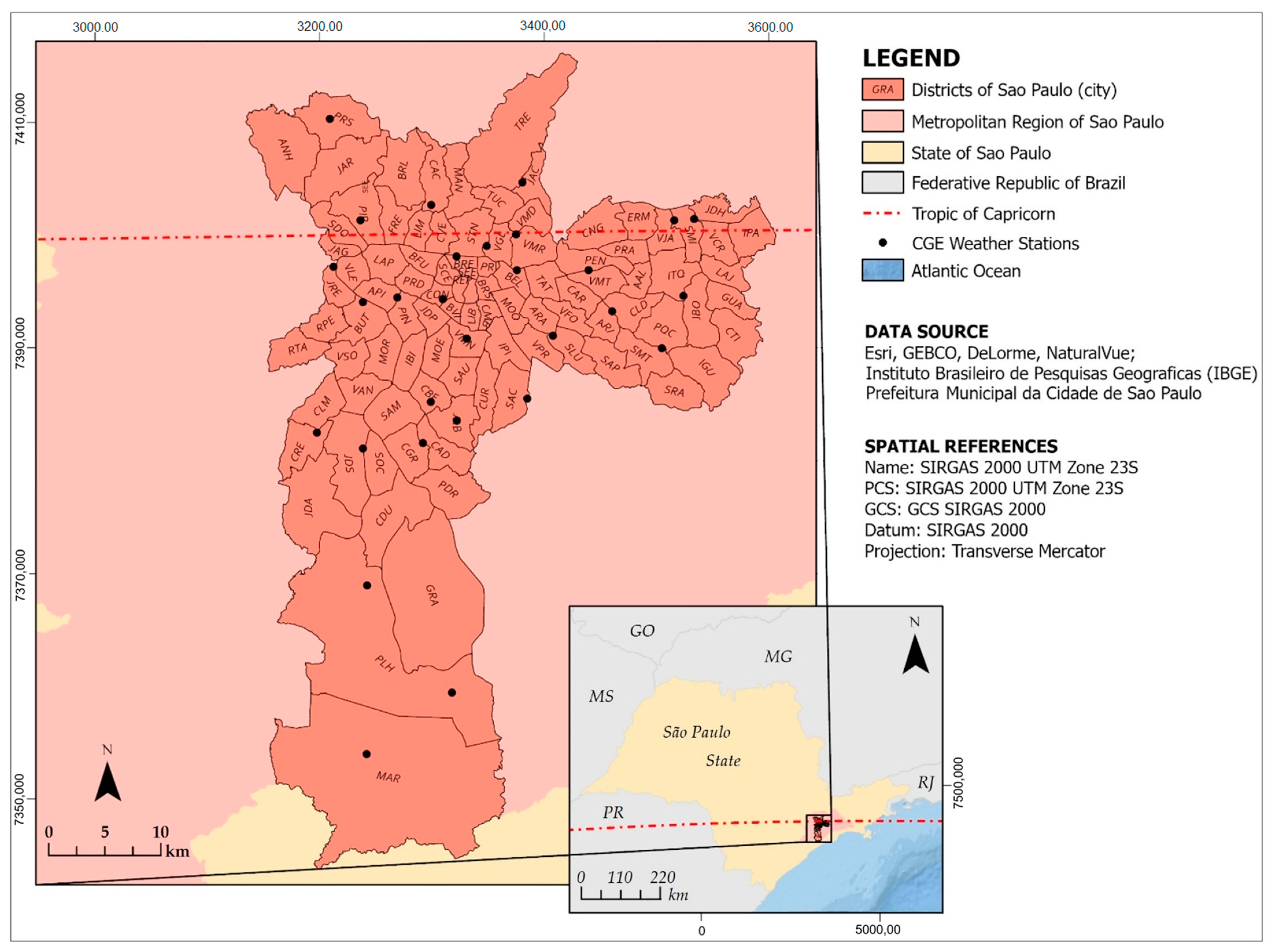
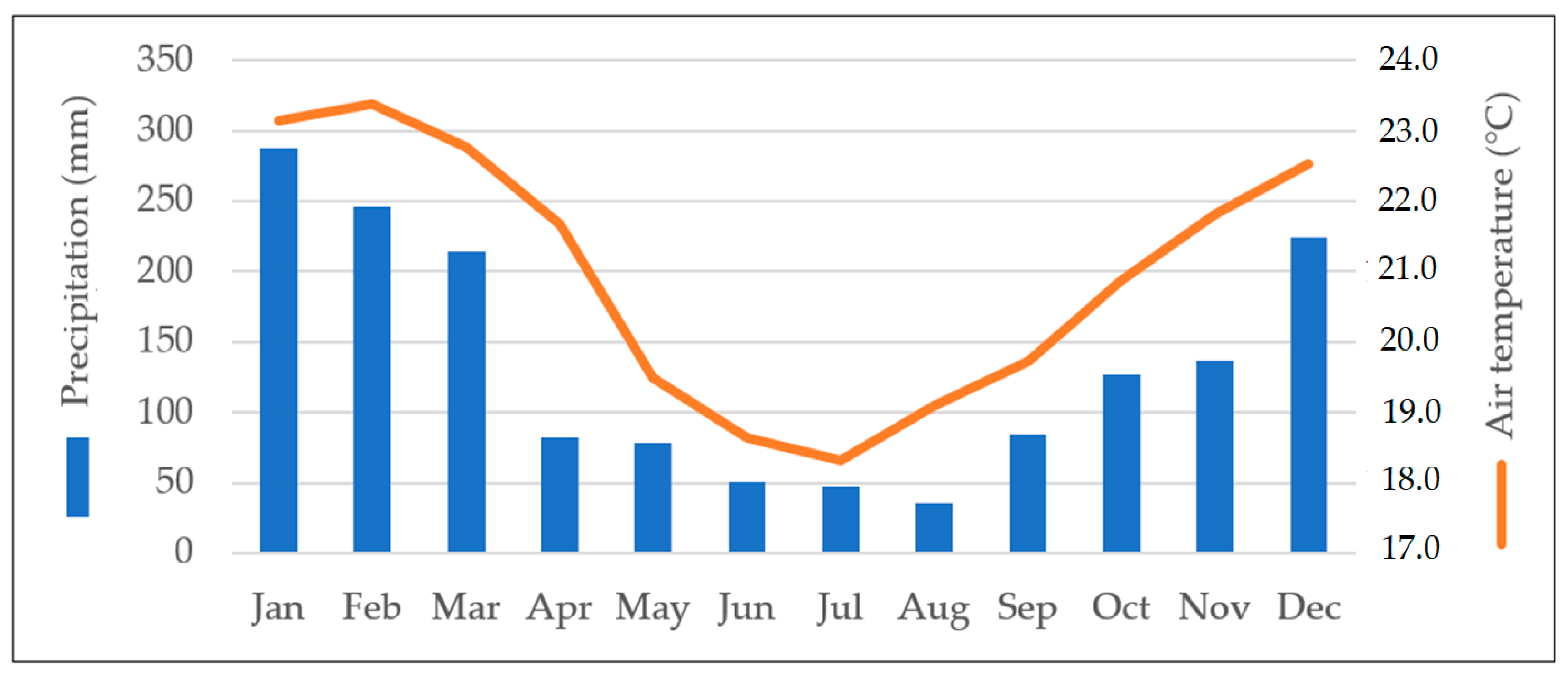
2. Characteristics of the Area of Study: São Paulo/SP

The city of São Paulo (Figure 1), located in the southeast region in Brazil, is the administrative capital of the state of São Paulo and acts as the central city of the Metropolitan Region of São Paulo (RMSP), which integrates 39 municipalities. The city of São Paulo has more than 12 million inhabitants and is 1521 km2 [36]. It is divided into 96 districts, which are administratively grouped into 32 sub-municipalities (Table 1).
The city is in the domains of the regional biome or ecosystem called Atlantic Forest. In contrast to its dense urban area, the city also has important green areas, concentrated (75%) in the Capivari-Monos Environmental Protection Area (south) and in the Serra da Cantareira State Park (north) [37]. The distribution of urban afforestation, both with native and exotic species, is also uneven in the municipality: there are well-tree-lined streets and streets where vegetation is absent [38].
In a generic description, it can be historically said that “the local conditions of the São Paulo basin created a temperate climate in this city in the Tropic of Capricorn, whose better name would be tropical temperate by altitude, in contrast to the hot hinterland and to the tropical coast of the State” [39]. However, the relief arrangement of the municipality of São Paulo “contributes to increasing the intensity of the heat island as well as favoring the concentration of pollutants” [29].
Urban climate units should also be considered in the analysis; they are divided into two macroclimate units: the central urban climate and the peripheral climate [37]. The peripheral climatic is particularly important for heat island monitoring, once it is “extreme climate units, sometimes rivers of mud, dirt, and floods, sometimes unbearable heat, sometimes too cold” [37], almost without the minimum environmental conditions for the reproduction of life. In the remote sensing context, “these are the “urban climates”, that is, the extreme heat, evident in satellite images, or replaced by thermally “softer” areas of the high slopes of the hills, or by the shading of the valley bottoms” [37].
Figure 2 shows the monthly average variation of temperature and precipitation based on the climatological data of Mirante de Santana weather station for the city of São Paulo from the period of 1981 to 2010, presented in Table 2. It is important to note that the period of 1981 to 2010 does not represent normal climatological data according to the rule of the WMO once they established a 30 year period with defined time intervals (1091 to 1930, 1931 to 1990, and 1991 to 2022). In that way, the INMET of Brazil works with updated climatological history data, nominated as provisory normal climatological data of Mirante de Santana, covering the period of 1981 to 2010. The fourth normal climatological data series of Mirante de Santana, according to the rules of WMO (1991 to 2022), has not been yet published at the time of publication of this article.

3. Materials and Methods

The recorded and orthorectified Landsat-8′s scenes were obtained by the Earth Explorer Platform from United States Geological Survey (USGS) with a processing quality criterion of C1 (Level-1), that is, the radiometric and atmospheric correction parameters have not yet been performed. The four selected scenes have cloud cover below 5% and are located over the city of São Paulo, respective to the summer–spring (21 January 2021, 1:04 p.m.) and autumn–winter (18 July 2019, 1:04 p.m.) periods.
The scenes were passed through atmospheric, topographic corrections and panchromatic sharpening using the Semi-Automatic Classification Plugin (SCP) and the Grass Gis 7 tool i.topo.corr, both using the software QGIS 3.10. For the topographic correction, the following steps were applied: download of SRTM data from Empresa Brasileira de Pesquisa de Agropecuária (Embrapa) with 90 m pixel resolution, reprojecting the SRTM to the CRS, changing imagery datatype to 64 bit with the r.recode tool, and making the illumination dataset with the i.topo.corr.ill tool, both using Grass Gis 7 plug-in in the software QGIS 3.10. The two desktop applications were developed by the Open Source Geoespatial Foundation, stablished in Chicago, USA; the hardware used to process the applications belongs to the Department of Geography and the Department of Earth Sciences at the University of Bergen. Therefore, a mosaic combining each pair of scenes to create new merged imagery for each date was performed.

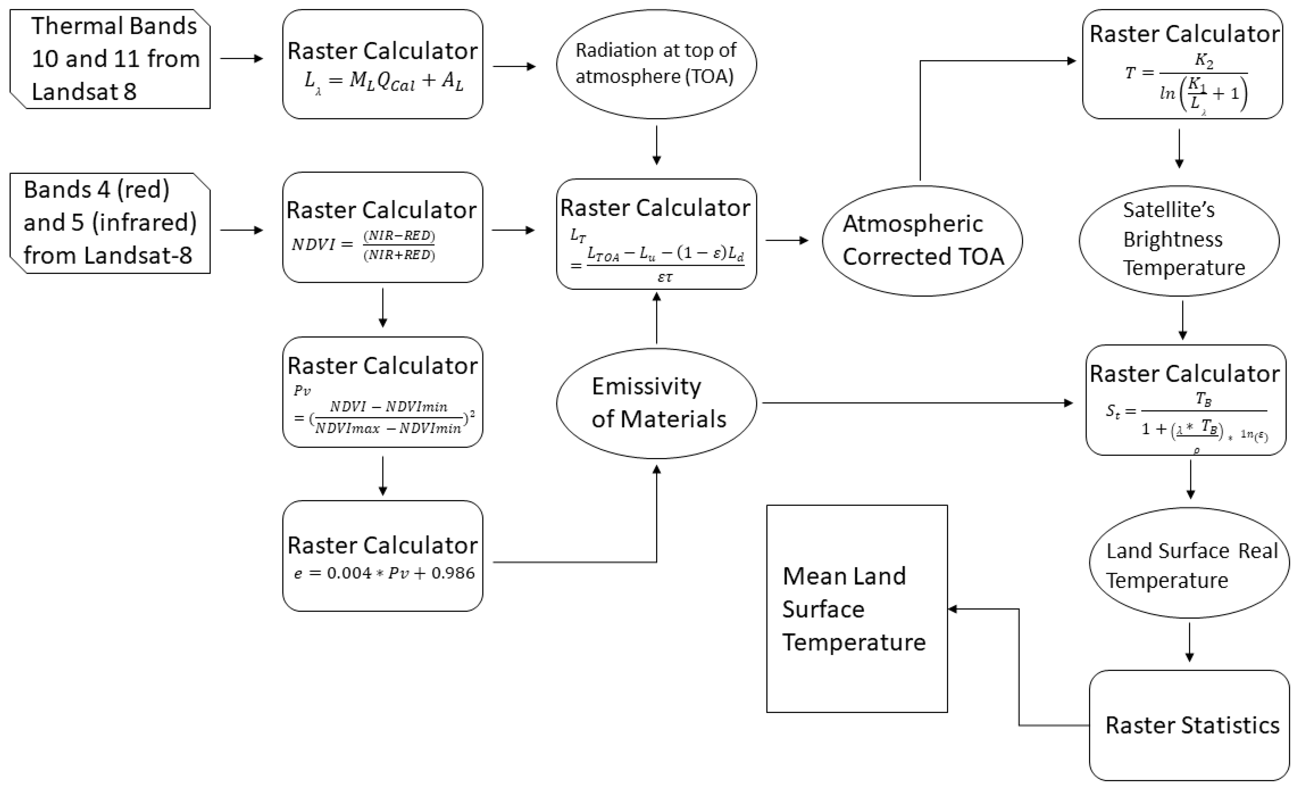
3.1. Land Surface Temperature Estimation

The TIRS instrument records the reflected energy radiance of the target and converts it to emitted energy radiance in addition to Stephen-Boltzman’s Law. The Arcmap (10.3.1) software will be used to convert energy-emitted radiance from thermal bands 10 and 11 into land surface temperature. Firstly, it is necessary to convert the digital number into radiation at the top of the atmosphere (TOA) using the radiance rescaling factors provided in the product metadata file (MTL file), according to Equation (1):
L λ = M L Q C a l + A L
in which, L λ is the spectral radiance at the top of the atmosphere, expressed in Wm 2   sr 1   μ m 1 ; M L is the multiplicative band of the metadata resizing factor, Q C a l is the standard value of quantified and calibrated product pixels, and A L is the additive band of the metadata resizing factor.
The second step is converting TOA spectral radiance to the radiance of a black body of kinetic temperature using the atmospheric correction method by the emissivity of the surface materials, according to Equation (2) [40]:
L T = L T O A L u ( 1 ε ) L d ε τ
in which, L T is the radiance of a black target of thermodynamic temperature, expressed in Wm 2   sr 1   μ m 1 ; L T O A is the spectral radiance at the top of the atmosphere, equivalent to L λ ; τ is atmosphere transmittance; ε is the emissivity of the surface; L u is the radiance emitted by the atmosphere in Wm 2   sr 1   μ m 1 ; e L d is the incident radiance on the surface in Wm 2   sr 1   μ m 1 .
The values of atmospheric transmittance, radiance emitted by the atmosphere, and surface incident radiance were calculated through the atmospheric correction calculator (WELBCALC) provided by the National Aeronautics and Space Administration (NASA). The input data (pressure, temperature, and relative humidity) was obtained from the database of the meteorological stations of the National Institute of Meteorology (INMET) from Brazil. The emissivity values were obtained through the NDVI (Equation (3)) that was converted into the proportion of vegetation (Equation (4)) and, finally, into deriving surface emissivity by Equation (5) [21]:
N DVI = ( NIR RED ) ( NIR + RED )
P v = ( NDVI NDVI m i n NDVI m a x NDVI m i n ) ²
e = 0.004 P v + 0.986
in which NIR refers to band 5 and RED to band 4 of the Operational Terra Imager (OLI) from the Landsat 8 satellite, as mentioned, after passed through atmospheric, topographic corrections and panchromatic sharpening.
In the third step, it is necessary to transform the atmospheric-corrected TOA spectral radiance ( L T ) to the satellite’s brightness temperature using the thermal constants available in the metadata file, according to Equation (6):
T = K 2 l n ( K 1 L λ + 1 )
in which T is the satellite’s brightness temperature expressed in Kelvin (K), and K 1 and K 2 are metadata conversion constants to the thermal images found in the metadata file.
After estimating the satellite’s brightness temperature, it is possible to establish the land surface real temperature with Equation (7). The algorithm chosen to perform the calculation was the single channel. “Single-channel methods still need to be explored and improved; however, it is the only hope for creating a global LST product for the entire Landsat thermal archive” [41], even though it presents uncertainty compared to split-window algorithms, which, in turn, requires atmospheric water vapor content data, which are not easy to get.
S t = T B 1 + ( λ   T B ρ )   1 n ( ε )
in which, T B is the brightness temperature; λ is the wavelength of emitted radiance ( 11.5   μ m ); ρ = h x ( c σ ) = 1.438     10 2   ( mK ) , in which σ is the Boltzmann’s constant ( 1.38     10 23   JK 1 ); h is the Planck’s constant ( 6626     10 34   Js ); c is the speed of light ( 2998     10   8   ms 1 ); ε is the emissivity in the area.
Finally, using the cell statistics tool with input as the LST of thermal bands 10 and 11, it was possible to obtain as output the mean value of the land surface temperature for the two respective dates. The flowchart of the procedures can be seen in Figure 3.

3.2. Correlative Analysis between Land Surface Temperature and Air Temperature

The existing correlation between the data obtained by sensors and by weather stations will be identified according to existing methodology [25]. The weather station locations are georeferenced and plotted into the LST spatialization; then, the LST values in the point of the weather stations are extracted into a table.
The interpolations are evaluated by means of cross-validation, where the mean absolute error (MAE) and the root mean square deviation (RMSD) are calculated, a methodology used to assess the degree of similarity between prediction and observation (Equation (9)).
MAE = 1 n   ( T e T o )
RMSD = 1 n   ( T e T o )   ²
in which To corresponds to the observed temperature (°C), Te to the estimated temperature (°C), and n to the number of monitoring stations. The calculations were performed in spreadsheets of Microsoft Excel (2013). Simple mean calculations for the values of air temperature, relative humidity and rainfall, and standard deviation, variation, and regression and the Pearson correlation coefficient between air temperature and LST were performed as well.
As the scene captured by the satellite occurred at 1:04 p.m., the best methodology to establish air temperature, pluviosity, and humidity from weather stations at the instant of the satellite scene is the mean of the previous (1:00 p.m.) and the subsequent (1:10 p.m.) instant recorded at the CGE’s weather stations. Consequently, new values are established for each of the 29 CGE’s weather stations, categorized as the mean estimated air temperature of the instant.
Thereafter, the statistical analysis, measured values, and estimated mean values are compared at each one of the 29 CGE’s weather stations within the city of São Paulo (the monitoring points Riacho Grande, Mauá-Paço Municipal, and Santana do Parnaíba are located outside the city). An average of –3.0 °C > x > 3.0 °C between differences of air temperature and LST to have satisfactory results for scientific research [27]. This difference was established due the transport of energy from the land surface to the temperature probe of the weather station (1.5 m) [27].

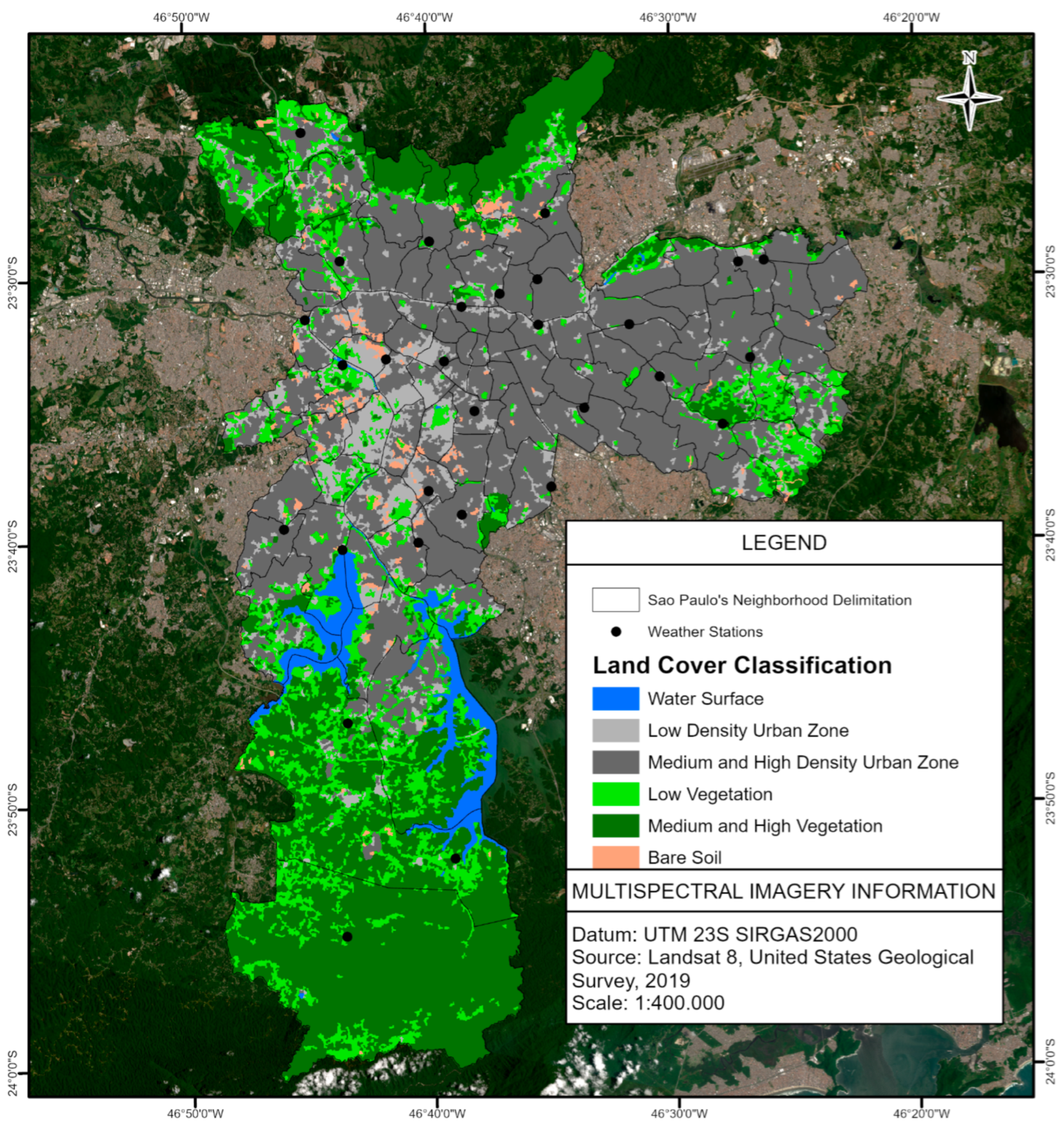
3.3. Land Use/Land Cover (LULC) Classification

The supervised classification was performed in QGIS using the Same-Automatic Classification Plugin (SCP), having as input the bands 2, 3, 4, 5, 6, and 7 of the Landsat 8 satellite and a training sample with at least one hundred clusters for each one of the classes established: bare soil, water surface, high and medium vegetation (density), low vegetation (density), high and medium urban zone (density), and low urban zone (density).
The algorithm chosen was the spectral angle mapper (SAM), which is a physically based spectral classification that uses an n-dimensional angle to match pixels to reference spectra, determining the spectral similarity between two spectra by calculating the angle between the spectra, treating them as vectors in a space with dimensionality equal to the number of bands [42]. The algorithm is relatively insensitive to illumination and albedo effects, which can help the classification in dense urbanized environments.
The classification, however, has a low level of generalization, making necessary the application of generalization processes for more suitable LULC mapping. Firstly, the wrongly classified pixels are removed, the boundaries between classes are smoothed, allowing smaller zones to expand and invade the limit of larger zones, and the pixels are divided and grouped into regions. Finally, a mask can be created in which pixels with count values less than 200 are encoded as NULL, so that the smaller regions can be excluded through a nibble process.

4. Results and Discussion

Before going further to any correlation analysis of land surface temperature, air temperature, and spatial and seasonal distribution, the limitations of the Landsat 8 temporal resolution and the cloud coverage in the intertropical region, where most of Brazil’s land is placed in the globe, will be discussed. Regarding the temporal resolution, the Landsat 8 long term acquisition plan says that “each satellite makes a complete orbit every 99 min, completes about 14 full orbits each day, and crosses every point on Earth once every 16 days”, which means that approximately 22 images are taken from the same point on Earth yearly, an average of 5 images per season. Researching the cloud cover seasonal variability in the croplands of South America, Prudente et al. (2020) discovered that 56% of Brazilian croplands have in between 50% to 60% cloud cover during September–November, 59% of the croplands have a cloud cover of 60% up to 80% during December–February, and 36% of the croplands have cloud cover from 40% to 50% in March–May; in June–August, 46% of the croplands have cloud coverage from 10% to 30%. São Paulo’s cloud cover scenario, as part of the intertropical region of Brazil, follows the country’s trend.
In that way, providing a time-series seasonal analysis with one single satellite is a difficult quest to achieve as the source may be unable to provide enough useful satellite images. However, it does not discredit all the research trying to achieve good remote sensing parameters and analysis methodology for Earth’s observations, as with this one, as the collaboration for the elaboration of a constellation of satellites and methodologies to acquire and manipulate reliable spatial data is the ultimate goal. Thus, the Landsat 8 satellite should not be the only one used for the time-series analysis of LST; it should be part of a constellation of satellites.

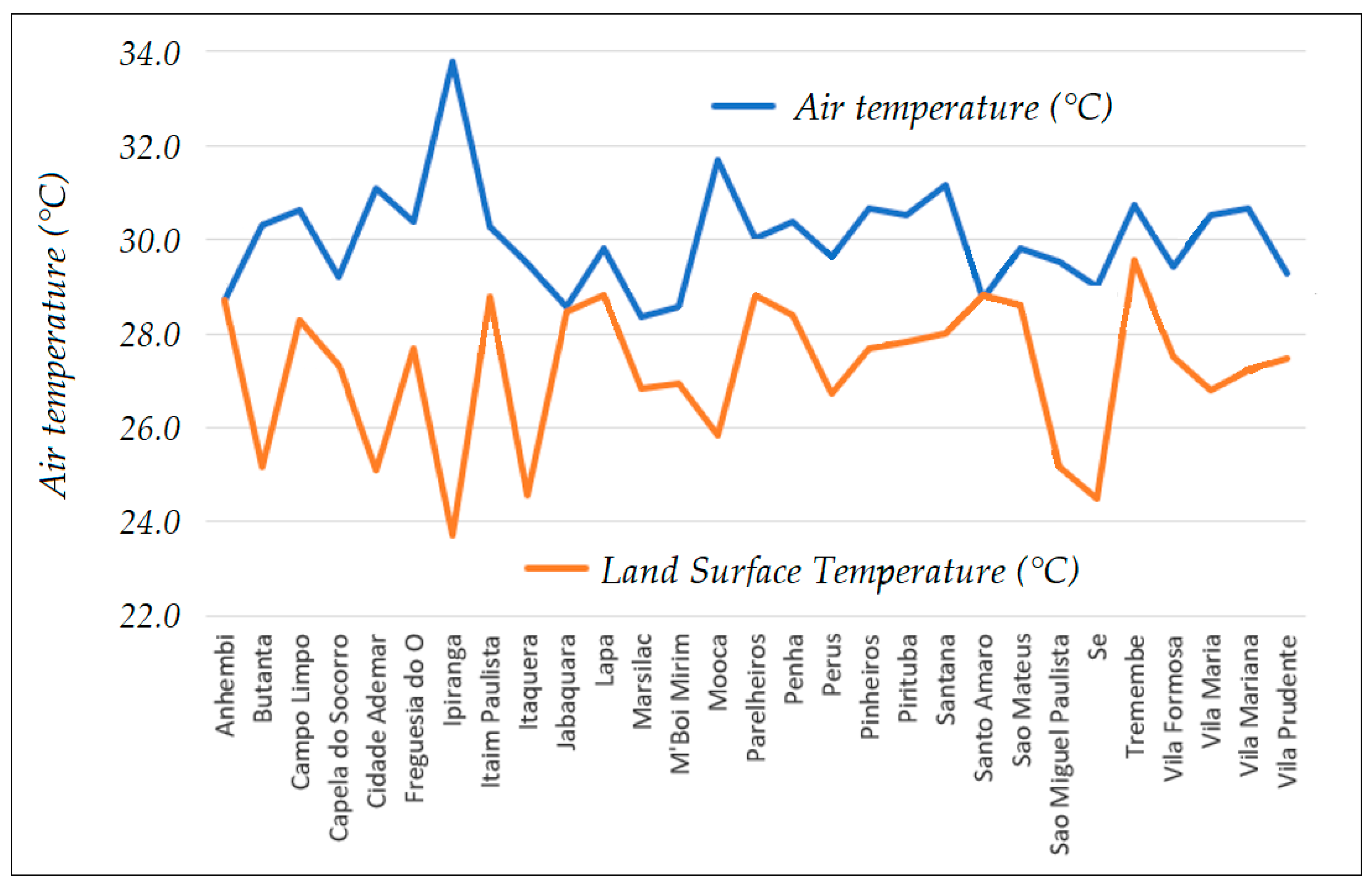
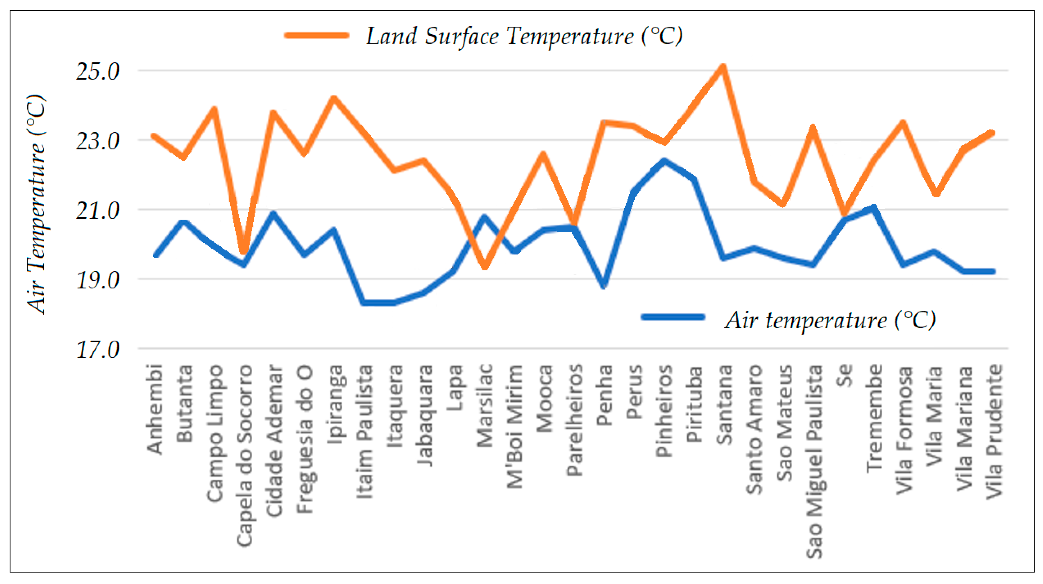
4.1. Correlation in between Land Surface Temperature and Air Temperature

The air temperature was obtained from the 29 weather stations of the CGE within the city of São Paulo. From the measurements, which are taken every 10 min, it was obtained the hourly mean corresponding to the instant at which the Landsat-8 satellite images were obtained, that is, the mean air temperature of 1:00 p.m. and 1:10 p.m. In this way, it is possible to cross-compare the LST values with air temperature, as shown in Figure 4 and Figure 5.
In the spring–summer period, most of the estimated values remain below the measured values, besides the weather stations of Anhembi, Jabaquara, and Santo Amaro, which have estimated values matching the observed values. The LST thermic amplitude is 5.9 °C as artificial surface coverage, buildings, and human activities, reflected in the mosaic of land occupation, significantly modify the radiation components of the energy balance throughout the city [6,7,8,9,10], with the minimum temperature at weather station Ipiranga (23.7 °C) and the maximum temperature at weather station Tremembé (29.6 °C).
In the autumn-winter period, most of the LST values are above the air temperature values, except in the weather stations of Marsilac, where the LST presents a value below the air temperature, most probably due to the release of heat and the increase of evapotranspiration processes and latent heat fluxes on this highly vegetated area [11,12,13,14] that decreased the emitted radiance to the satellite. The LST thermic amplitude is 6.1 °C, with the minimum value at weather station Marsilac (19.3 °C) and the maximum value at weather station Santana (25.1 °C).
The LULC’s and surface emissivity’s influence on the variation in temperatures is very strong since it follows similar trend lines on both dates. They have higher temperatures at Campo Limpo, Penha, Santana, Itaim Paulista, and Itaquera weather stations and lower temperatures at the Capela do Socorro, Marsilac, Parelheiros, M’Boi Mirim, and Lapa weather stations. It is clear, then, that the modifications imposed by the city’s shape on the local climate system affect the city’s inhabitants and expose them to the consequences of urban heat islands and thermal discomfort [4,17].
The air temperature shows no trend lines as there are other variables in its measurements of wind direction and speed, humidity, and rainfall. Besides that, the CGE meteorological stations do not meet the criteria established by the INMET—a flat location to avoid the accumulation of water and far from electrical installations; broad horizons, without barriers that prevent solar radiation or change the characteristics of the wind; distance from watercourses and grassy or undergrowth soil—compromising the results and measurements. They are placed throughout the city in the most diverse types of terrains: above liquid surfaces, on concrete, on asphalt, under dense vegetation, and so forth, and this negatively affects the reliability, efficiency, and fidelity of the results.
The values of the mean absolute error (MAE) and root mean square deviation (RMSD) of the temperature estimated by the observed temperature, as well as the mean of the difference between LST and air temperature and the standard deviation for each of the 29 meteorological stations of the CGE on both dates, can be seen in Table 3 and Table 4.
The LST is 2.8 °C lower in spring–summer and 2.6 °C higher in autumn–winter on average; however, adding the standard deviation of 2.2 °C in spring–summer and 1.5 °C in autumn–winter, 95% of the samples have differences in between −4.9 and −0.6 °C in spring–summer and 4.1 and 1.1 °C in autumn–winter. Using the stablish difference interval of −3.0 °C > x > 3.0 °C for the values of LST and air temperature [43], the spring–summer season presents 72.0% of satisfactory values, while the autumn–winter season presents 58.6% of the results in between −3.0 °C > x > 3.0 °C. However, applying the standard deviation of ±2.2 °C for spring–summer and ±1.5 °C for autumn–winter and considering the accuracy of ±0.2 °C of the HMP45C-L temperature and humidity probe from the CGE weather stations, the reliability of the results during the spring–summer period is up to 86.2% and during autumn–winter is up to 93.1%. The increase in reliability during winter is due “winter’s ability to homogenize the surrounding environment, which increases the reliability of the surface temperature to determine near-surface temperatures” [44].
The present work demonstrates satisfactory results compared to other literature. Gusso (2003) also showed a mean difference of 2.6 °C for autumn–winter measurements using the sensor AVHRR/NOAA, while Caselles et al. (1997) compared methods for LST estimation and found a mean difference of 4.0 °C in between LST and air temperature, while the highest mean difference in the current work is of 2.8 °C in January measurements. Wenbin et al. (2012) reached an RMSE ranging from 2.9 to 3.2 °C, and Vancutsem et al. (2010) found 75% of their results under 2.0 °C for MAE and 2.7 °C for RMSE by analyzing MODIS land surface products, while the mean MAE and mean RMSE from this present work ranges from 1.2 to 1.9 °C, with 82.7% of the values being ≤2.7 °C. Mutiibwa et al. (2015), nevertheless, found better results studying complex terrain in Nevada, USA, using MODIS technology, with a mean difference of 1.8 °C; however, there was a standard deviation of 7.7 °C; additionally, they discovered an interesting seasonal trending on the results: better accuracy in summer due clear-sky conditions and a poor relationship in winter due to prevalent clouds. The tropical temperate by altitude climate of the city of São Paulo [39] reveals a true inverse relationship as its summer presents high precipitation and the heavy presence of clouds, while its winter presents long dry periods with clear sky conditions. Analyzing previous literature on other satellites rather than MODIS, Hadria et al. (2017) discovered the mean values of 3.0 °C for RSME and 2.3 °C for MAE for the Advanced Very High Resolution Radiometer sensor on-board the National Oceanic and Atmospheric Administration’s satellites.
Using the software Excel (2013), the Pearson coefficient was calculated for both dates, being r = 0.81 for the spring–summer season and r = 0.82 for the autumn–winter season; however, the statistic results of MAE, RMSD, and difference (°C) are parameters with higher importance to the validation of the comparison between LST and air temperature. Gusso (2003), analyzing three different methodologies, calculated the results of R² = 0.73 to 0.77; Vancutsem et al. (2010) reached results from R² = 0.42 to 0.86; Mutiibwa et al. (2015) achieved the results of R² = 0.74 (winter), R² = 0.86 (spring), and R² = 0.92 (fall and summer). Wenbin et al. (2013) and Urban et al. (2013) preferred to work with the correlation coefficient, the first showing r = 0.83 to 0.94 and the second showing r = 0.89 from the (A)ATSR satellite, r = 0.90 from the AVHRR Polar Pathfinder, and r = 0.95 from MODIS Terra and Aqua. The results of the current work are lower than the ones showed by Gusso (2003) and Mutiibwa et al. (2015); however, our results are close to some of the results showed by Wenbin et al. (2013) and Urban et al. (2013) and even higher than some of the results showed by Vancutsem et al. (2010).

4.2. Correlation in between Land Surface Temperature and LULC

The LULC map (Figure 6) shows the existence of areas with high vegetation coverage in the south and north regions of the city of São Paulo: Serra do Mar State Park and Cantareira State Park. The urban area is concentrated in between the parks and extends to the East Zone. Some low vegetation spots can also be seen in the west–south axis and in the extreme east, respective to the Santa Helena Park (Figure 6).
Regarding the urbanized area, there is a lower density of urbanization in the west–south axis, in a strip that separates the old center from the east of the city and in the nort–west area, taking advantage of the vegetation corridors from the Cantareira State Park. The medium and high urban zones cover most of the urbanized areas in the city, being the predominant land use in the north, east, and southeast axis, showing a higher level of degradation in the environment and, consequently, in the quality of life of its citizens [16].
The relationship between the LULC classification and LST is clear: areas with a higher density of urban occupation have higher temperatures, followed by areas of low density of urban occupation and low vegetation cover/pastures, and areas with high vegetation cover and liquid surfaces (e.g., rivers, lakes, streams, dams) with lowest temperatures. The first two areas with urban occupation can be designated as built-up areas, while the other two areas can be designated as rural areas. Regarding the built-up area, the difference in temperature between higher-density urban occupation and low-density urban occupation is clear, the first being known as heat islands and the second as freshness islands. Thus, the uneven distribution of green areas and the densely concentrated demographic population generate multiple heat islands that have negative effects on urban areas [32,33,34,35], with occasional and rare freshness islands. The LST estimations are shown in Figure 7 and Figure 8.
Comparing the present LST mapping with the one presented in the 2002 Environmental Atlas of the City of São Paulo is possible in order to verify that the central–west–south axis upscale neighborhoods have maintained their mild temperatures since the years of 1999/2000, including areas with high urban density. In contrast, the urban heat island has been expanding to the East Zone, North Zone, and South Zone, sometimes invading areas that previously belonged to State Parks, permanent protection areas (APPs), and environmental protection areas (APAs) [26].
The urban heat island is displaced through most of the built-up space in the city of São Paulo, being confined by the rural areas of vegetation and water bodies’ surfaces in the north, east, and south and by the freshness island downtown, with its effects cooling the effects spreading to the west. The high-density urban zone in between the two biggest water surfaces (Guarapiranga Dam and Billings Dam), in the area known as “further-South”, can be wrongly mistaken as a freshness island as it presents colder temperatures compared to other high-density urban zones in the city. However, compared to the 1999/2000 mapping [26], that area used to be classified as a vegetation surface, presenting colder LST, as, nowadays, it is a heat island with less intensity, proving that changes in urban LULC intensify climate change and that urban expansion has a significant impact on land and surface temperatures.
In that way, the north–east–south heat island has, on average, temperatures varying from 28.4 to 32.9 °C during spring–summer and from 21.6 to 25.8 °C during autumn–winter; the further-South heat island presents LSTs varying from 27.1 to 29.4 °C during spring–summer and from 21.6 to 25.8 °C in autumn–winter. The downtown-West freshness island shows LST ranges in spring-summer of mainly 25.6 to 27.0 °C, with small areas ranging from 23.8 to 25.5 °C and from 27.1 to 28.3 °C, while in autumn–winter, it ranges from 19.4 to 23.6 °C. The rural area (vegetation and water bodies) ranges from 21.5 to 25.5 °C during spring–summer and from 17.3 to 21.5 °C during autumn–winter.
The autumn–winter LST is well and sparsely distributed on the whole territory, with the presence of notorious overlapping LST ranges in vast areas in between rural areas and the freshness island and in between the freshness island and heat islands. In both the rural and freshness islands, it is possible to visualize vast extensions of land with LSTs from 19.4 to 21.5 °C; big regions, either in the freshness island or heat island, with temperatures ranging from 21.6 to 23.6 °C, are also visible. However, during the spring-summer period, the thermal amplitude is stronger and presents considerable differences in temperature in between the rural areas, freshness island areas, and heat island areas.
Therefore, air temperature in the far east zone, both provided by the CGE, differs from the temperature estimated by remote sensing and the peripheral urban climate characterization [26], since, in summer, there were milder temperatures, which may indicate a measurement error in the thermometers of the CGE’s weather stations or that the region is in another urbanization process and requires an update regarding its microclimate as it does not show the characteristic “extreme heat”.
The urbanization and peripheral expansion produced microclimates for the city based on the different techniques and technologies used: the presence of buildings, materials unsuitable for civil construction, public roads that absorb large amounts of solar radiation, reduced wind speed and change of direction by buildings and towers, pollution that reduces the loss of long-wave radiation from surfaces to the sky, rainwater catchment systems with insufficient drainage, the use of impermeable coatings on the ground, and the reduction of energy used in evapotranspiration processes performed by vegetation [42]. Green areas, in turn, are concentrated in a few places, presenting local effects instead of being proportionally distributed over the built-up space.

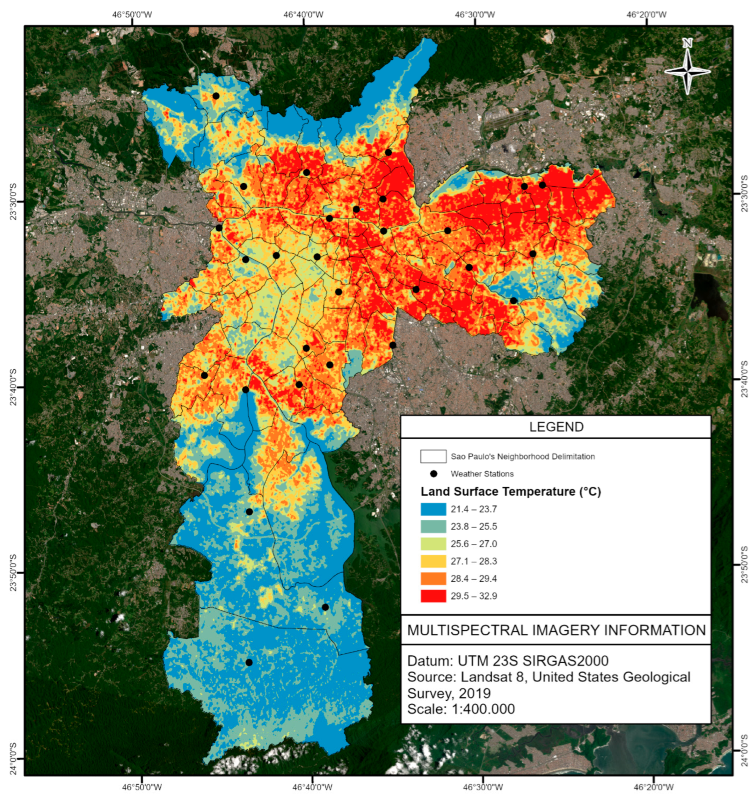
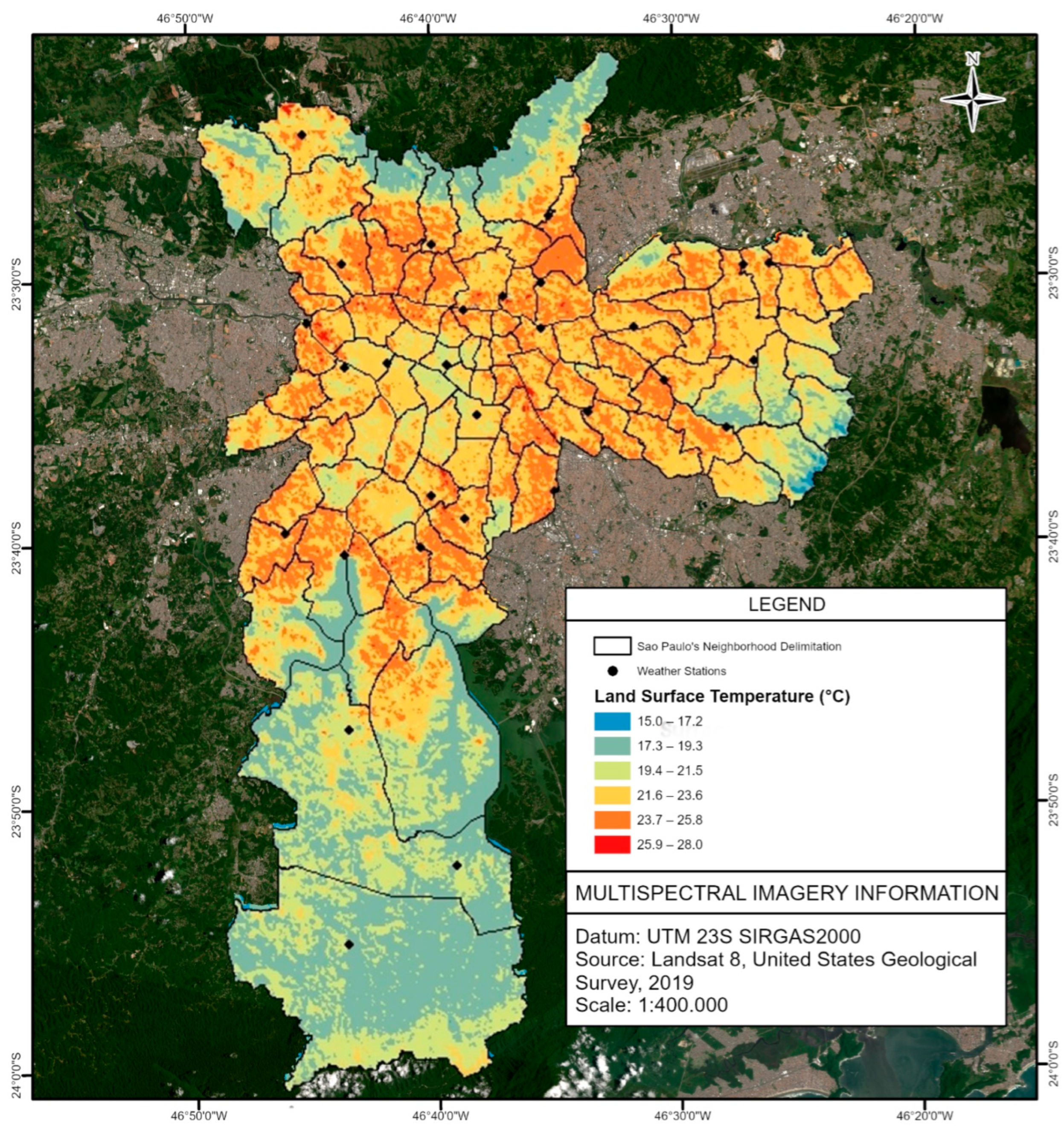
4.3. Land Use/Land Cover and Seasonality Impact

The troubled mosaic of the metropolitan region of São Paulo presents “surface conditions, changes to the soil moisture content, and heterogeneity of the LULC can play a major role in determining the variations between seasons” [44]. Additionally, the 16-day time resolution for Landsat-8 and the lack of a cloud mask algorithm limit the availability of data [44]. Furthermore, the 30 m pixel OLI sensor and the 15 m panchromatic band are neither precise enough to categorize the LULC of the city correctly nor broad enough to homogenize the LULC categories; this is a disadvantage.
The comparison results from weather stations placed over or near water bodies and vegetated covers within urban areas are the most discrepant as non-evaporating surfaces present higher temperatures, while liquid and vegetated surfaces present lower temperatures due to radiant reflection and soil transpiration [43]. To boot, the reflected solar radiation on the impervious pixels can impact the LST strongly [44].
Analyzing Figure 7 and Figure 8, both periods, spring–summer and autumn–winter, present similar spatial distributions of hot and fresh zones throughout the city; however, a difference in the intensity of the heat islands when comparing the spring–summer LST (Figure 7) and the autumn–winter LST (Figure 8) is visible. Having as a reference the freshness island of the high upright downtown and the hot islands of the north–east axes, during the autumn–winter season, the LST in both regions differs on average 4.2 °C, while during spring–summer season, the LST differs on average 7.3 °C, with points that can have a difference of up to 9.1 °C.
When comparing the rural region with lowest values of LST with the heat islands of the north–east axis, the difference in LST temperatures in between climatological periods can be, on average, from 4.4 to 8.5 °C for the autumn–winter season. The values are significantly higher in the spring–summer season, ranging from 5.8 up to 11.5 °C. The highest thermal amplitude during spring–summer can be directly linked to the land use/land cover of the city of São Paulo, especially in the low-income neighborhoods (low–middle class and poor suburbs) of the North Zone and the East Zone, with intense urbanization and low arborization, commonly with the presence of self-construction houses with improper materials [26].
In addition, the lowest and highest temperatures during the autumn–winter period are only shown in small areas, almost not visible through eye inspection, mainly located on the border of the image. It can probably be designated to two factors: geoprocessing error on the border of the images due to clipping processes and/or unusual materials on the surface as laminated metal roofs or deep lagoons, and so forth.

5. Conclusions

  • The correlation in between LST and air temperature indicates a similar spatial distribution pattern as regions classified as Medium and High Vegetation, Low Vegetation, and Water Surfaces hold low or mild temperatures, in contrast to the higher temperatures observed in Medium and High-Density Urban Zones. The formation of cold islands, probably caused by the projection of the shadows of buildings in areas with a higher pattern of vertical occupation, is predominantly found in the Low-Density Urban Zone. These cold islands are also observed in the areas of the so-called garden neighborhoods due to the predominance of horizontal residential occupation and intense urban afforestation. Furthermore, it is possible to relate the influence of the materials found on the surfaces registered by the thermal sensor, that is, the emissivity of the materials and the respectively revealed apparent temperatures.
  • The North–East–South heat island has temperatures varying from 28.4 to 32.9 °C during spring–summer and from 21.6 to 25.8 °C during autumn–winter; the further-South heat island presents LSTs varying from 27.1 to 29.4 °C during spring–summer and from 21.6 to 25.8 °C in autumn–winter. The downtown-West freshness island shows LST ranges in spring–summer of mainly 25.6 to 27.0 °C, with small areas ranging from 23.8 to 25.5 °C and from 27.1 to 28.3 °C, while in autumn–winter, it ranges from 19.4 to 23.6 °C. The rural area (vegetation and water bodies) ranges from 21.5 to 25.5 °C during spring–summer and from 17.3 to 21.5 °C during autumn–winter. The autumn–winter LST is well and sparsely distributed over the whole territory, with the presence of notorious overlapping LST ranges in big areas in between rural areas and the freshness island and in between the freshness island and heat islands. In both rural and freshness islands, it is possible to visualize vast extensions of land with LSTs from 19.4 to 21.5 °C; notorious regions, either in the freshness island or heat island, with temperatures ranging from 21.6 to 23.6 °C, are also visible. However, during the spring-summer period, the thermal amplitude is stronger and presents considerable differences in temperature in between rural areas, freshness island areas, and heat island areas. The thermal amplitude can range from 4.4 to 8.5 °C for the autumn–winter season and from 5.8 up to 11.5 °C in the spring–summer season.
  • The CGE weather stations aim to monitor the weather in order to minimize the extreme weather hazards as they do not meet the criteria established by the WMO: a flat location to avoid the accumulation of water and far from electrical installations; broad horizons, without barriers that prevent solar radiation or change the characteristics of the wind; distance from watercourses, grassy or undergrowth soil, and so forth. They are placed throughout the city in the most diverse types of terrains: above liquid surfaces, on concrete, on asphalt, under dense vegetation, and so forth. However, the stations present a temperature related to the emissivity of the materials along the city’s surface; in other words, they are particularly suitable for the comparison with LSTs estimated by satellites.
  • The Landsat 8′s TIRS sensor spatial resolution of 100 m compromises the quality of the land surface temperature estimation, especially considering the chaotic land use distribution in the megacity of São Paulo, where different surface materials are mixed and layered with each other: e.g., bridges over channelized rivers, urban gardens in between avenues. Thus, the emitted radiance of the materials read by the satellite is not trustworthy to the position of the weather stations, considering the pixel size. However, the 30 m spatial resolution OLI red and infrared bands were used to obtain surface emissivity, smoothing the pixel error of the thermal bands.
  • The LST results were satisfactory, especially in the January measurements, with 72.0% of the results being less than 3 °C higher or lower than the weather-station-collected data. Considering that the LST presents values below the air temperature, applying the standard deviation of ±2.2 °C and the accuracy of ±0.2 °C of the HMP45C-L temperature and humidity probe from the CGE weather stations, the differences between the measurements and estimations have up to 99.3% accuracy. It also shows a mean difference of −2.8 °C, a mean MAE of −1.4 °C, a mean RMSE of 2.0 °C, and a coefficient of determination R² = 0.83. Those values are in accordance and are satisfactory, considering the other works published.
  • The measurements in August presents, initially, only 58.6% of results of less than 3.0 °C higher or lower temperatures than the observed data of CGE. However, considering that the LST values are mainly above the air temperature, when applying its standard deviation of ±1.5 °C and the HMP45C-L accuracy error of ±0.2 °C, the difference estimation of air temperature by LST is highly accurate, within 93.1%. It also shows a mean difference of 2.6 °C, a mean MAE of 1.2 °C, a mean RMSE of 1.8 °C, and a coefficient of determination R² = 0.63. The coefficient of determination is slightly under the overall results of the literature compared; however, it still presents better results compared to some of Vancutsem et al. (2010) analyses.
  • Providing a time-series seasonal analysis with a single satellite is a difficult quest to achieve as the source may be unable to provide enough useful satellite images due to the temporal resolution and the cloud coverage on the intertropical region, especially during the rainy season. However, it does not discredit all the research trying to achieve good remote sensing parameters and analysis methodology for Earth observations, as with this one, as the collaboration for the elaboration of a constellation of satellites and methodologies to acquire and manipulate reliable spatial data is the ultimate goal. Thus, the Landsat 8 satellite should not be the only one used for the time-series analysis of LST; it should be a part of a constellation of satellites.
  • Acquiring meteorological data for a historical LST comparison analysis of the city of São Paulo during the pandemic scenario in Brazil is a difficult barrier to break. The data from CGE during the months of January and August of 2019 were acquired in the same year as it is stored and freely available for a short period of time. Requiring past data is a bureaucratic and long process even in normal conditions: we need a letter of request for the CGE data from the university; we need to apply the request data to the CGE platform, send all the necessary documentation as a preview of the research, wait for the approval, and then wait for the data to be sent. Those processes during the pandemic could have taken months as many governmental units were closed or paused from a lack of employees. However, it is an interesting approach for future research.
  • The correlation of the land urban heat and freshness/cold islands with LULC and seasonality was initially done in this current work through the LST analysis as it was possible to visualize the distribution of land surface heat on the city. Further, starting from this current work, new measurements in the intensity of the surface urban heat island (UHI) effect can be done, applying the temperature difference index, the UHI effect classification index, and the urban thermal field variance index (UFTVI) of SUHI.

Author Contributions

Conceptualization, A.C.L.d.N. and E.G.; methodology, A.C.L.d.N. and E.G.; software, A.C.L.d.N.; validation, A.C.L.d.N., E.G., J.P.A.G. and C.A.W.; formal analysis, A.C.L.d.N., J.P.A.G. and C.A.W.; investigation, A.C.L.d.N. and E.G.; resources, A.C.L.d.N., E.G. and C.A.W.; data curation, A.C.L.d.N.; E.G. and J.P.A.G.; writing—original draft preparation, A.C.L.d.N., E.G., J.P.A.G. and C.A.W.; writing—review and editing, A.C.L.d.N., J.P.A.G. and C.A.W.; visualization, A.C.L.d.N., J.P.A.G. and C.A.W.; supervision, A.C.L.d.N., J.P.A.G. and C.A.W.; project administration, A.C.L.d.N.; funding acquisition, A.C.L.d.N., E.G. and C.A.W. All authors have read and agreed to the published version of the manuscript.

Funding

This research received no external funding.

Institutional Review Board Statement

Not applicable.

Informed Consent Statement

Not applicable.

Data Availability Statement

Not applicable.

Acknowledgments

We thank the Agência USP de Inovação for providing the research AUSPIN entrepreneur scholarship; we thank Márcia Cassemiro and Vivian de Castro from the Comissão de Cooperação Internacional from the Faculty of Philosophy, Literature and Human Sciences (FFLCH) for helping throughout the exchange program; we thank Hans Peter Anderson and Benjamin Aubrey Robson for welcoming our researcher to the University of Bergen; we also thank the Conselho Nacional de Desenvolvimento Científico e Tecnológico (CNPq) for proving the Research and Productivity research grant (process number 304973/2017-3 and 306505/2020-7).

Conflicts of Interest

The authors declare no conflict of interest.

References

  1. Kandya, A.; Mohan, M. Mitigating the Urban Heat Island effect through building envelope modifications. Energy Build. 2018, 164, 266–277. [Google Scholar] [CrossRef]
  2. Gobo, J.P.A.; Faria, M.R.; Galvani, E.; Goncalves, F.L.T.; Monteiro, L.M. Empirical Model of Human Thermal Comfort in Subtropical Climates: A First Approach to the Brazilian Subtropical Index (BSI). Atmosphere 2018, 9, 391. [Google Scholar] [CrossRef] [Green Version]
  3. Gobo, J.P.A.; Faria, M.R.; Galvani, E.; Amorim, M.C.C.T.; Celuppi, M.C.; Wollmann, C.A. Empirical Model of Thermal Comfort for Medium-Sized Cities in Subtropical Climate. Atmosphere 2019, 10, 576. [Google Scholar] [CrossRef] [Green Version]
  4. Gobo, J.P.A.; Wollmann, C.A.; Celuppi, M.C.; Galvani, E.; Faria, M.R.; Mendes, D.; Oliveira-Júnior, J.F.; Malheiros, T.F.; Riffel, E.S.; Gonçalves, F.L.T. The bioclimate present and future in the state of São Paulo/Brazil: Space-time analysis of human thermal comfort. Sustain. Cities Soc. 2021, 78, 103611. [Google Scholar] [CrossRef]
  5. Wollmann, C.A.; Hoppe, I.L.; Gobo, J.P.A.; Simioni, J.P.D.; Costa, I.T.; Baratto, J.; Shooshtarian, S. Thermo-Hygrometric Variability on Waterfronts in Negative Radiation Balance: A Case Study of Balneário Camboriú/SC, Brazil. Atmosphere 2021, 12, 1453. [Google Scholar] [CrossRef]
  6. Litardo, J.; Palme, M.; Borbor-Cordova, M.; Caiza, R.; Macias, J.; Hidalgo-Leon, R.; Soriano, G. Urban Heat Island intensity and buildings’ energy needs in Duran, Ecuador: Simulation studies and proposal of mitigation strategies. Sustain. Cities Soc. 2020, 62, 102387. [Google Scholar] [CrossRef]
  7. Tian, L.; Li, Y.; Lu, J.; Wang, J. Review on Urban Heat Island in China: Methods, Its Impact on Buildings Energy Demand and Mitigation Strategies. Sustainability 2021, 13, 762. [Google Scholar] [CrossRef]
  8. Yang, X.; Jin, T.; Yao, L.; Zhu, C.; Peng, L.L. Assessing the Impact of Urban Heat Island Effect on Building Cooling Load based on the Local Climate Zone Scheme. Procedia Eng. 2017, 205, 2839–2846. [Google Scholar] [CrossRef]
  9. Yang, X.; Peng, L.L.H.; Jiang, Z.; Chen, Y.; Yao, L.; He, Y.; Xu, T. Impact of urban heat island on energy demand in buildings: Local climate zones in Nanjing. Appl. Energy 2020, 260, 114279. [Google Scholar] [CrossRef]
  10. Yang, X.; Yao, L.; Jin, T.; Peng, L.L.; Jiang, Z.; Hu, Z.; Ye, Y. Assessing the thermal behavior of different local climate zones in the Nanjing metropolis, China. Build. Environ. 2018, 137, 171–184. [Google Scholar] [CrossRef]
  11. Asaeda, T.; Ca, V.T.; Wake, A. Heat storage of pavement and its effect on the lower atmosphere. Atmospheric Environ. 1996, 30, 413–427. [Google Scholar] [CrossRef]
  12. Salata, F.; Golasi, I.; Vollaro, R.D.L.; Vollaro, A.D.L. Outdoor thermal comfort in the Mediterranean area. A transversal study in Rome, Italy. Build. Environ. 2016, 96, 46–61. [Google Scholar] [CrossRef]
  13. Thom, J.K.; Coutts, A.M.; Broadbent, A.M.; Tapper, N. The influence of increasing tree cover on mean radiant temperature across a mixed development suburb in Adelaide, Australia. Urban For. Urban Green. 2016, 20, 233–242. [Google Scholar] [CrossRef]
  14. Richards, D.R.; Fung, T.K.; Belcher, R.N.; Edwards, P.J. Differential air temperature cooling performance of urban vegetation types in the tropics. Urban For. Urban Green. 2020, 50, 126651. [Google Scholar] [CrossRef]
  15. Agopyan, V.; Jhon, V.M. O Desafio da Sustentabilidade na Construção Civil; Editora Blucher: São Paulo, Brazil, 2011; p. 144. [Google Scholar]
  16. Amorim, M.C.D.C.T. Ilhas de Calor Urbanas: Métodos e Técnicas de Análise. Rev. Bras. Clim. 2019, 22–46. [Google Scholar] [CrossRef] [Green Version]
  17. IPCC. Climate Change 2014: Synthesis Report. Contribution of Working Groups I, II and III to the Fifth Assessment Report of the Intergovernmental Panel on Climate Change; Pachauri, R.K., Meyeer, L.A., Eds.; United Nations: Geneva, Switzerland, 2014. [Google Scholar]
  18. SOARES, F.S.; Almeida, R.K.; Rubim, I.B.; Barros, R.S.; Cruz, C.B.M.; Mello, G.V.; Neto, J.A.B. Análise comparativa da correção atmosférica de imagem do Landsat 8: O uso do 6S e do ATCOR2. In Proceedings of the Simpósio Brasileiro de Sensoriamento Remoto, 17, (SBSR), João Pessoa, Brazil, 25–29 April 2015; Instituto Nacional de Pesquisas Espaciais (INPE): João Pessoa, Brazil, 2015; pp. 1821–1828. Available online: http://www.dsr.inpe.br/sbsr2015/files/p0358.pdf (accessed on 29 December 2021).
  19. Gusso, A.; Fontana, D.C.; Gonçalves, G.A. Mapeamento da temperatura da superfície terrestre com uso do sensor AVHRR/NOAA. Pesqui. Agropecuária Bras. 2007, 42, 231–237. [Google Scholar] [CrossRef]
  20. Wang, M.; He, G.; Zhang, Z.; Wang, G.; Wang, Z.; Yin, R.; Cui, S.; Wu, Z.; Cao, X. A radiance-based split-window algorithm for land surface temperature retrieval: Theory and application to MODIS data. Int. J. Appl. Earth Obs. Geoinf. 2019, 76, 204–217. [Google Scholar] [CrossRef]
  21. Valor, E.; Caselles, V. Mapping land surface emissivity from NDVI: Application to European, African, and South American areas. Remote Sens. Environ. 1996, 57, 167–184. [Google Scholar] [CrossRef]
  22. Shafri, H.Z.M.; Suhaili, A.; Mansor, S. The Performance of Maximum Likelihood, Spectral Angle Mapper, Neural Network and Decision Tree Classifiers in Hyperspectral Image Analysis. J. Comput. Sci. 2007, 3, 419–423. [Google Scholar] [CrossRef] [Green Version]
  23. Maia, M.A.; Rodrigues, N.B.; Richter, M.; Rubim, I.B. Modelos de correção atmosférica aplicados em imagens OLI/Landsat 8 a partir do uso de programas gratuitos: Uma análise comparativa. In Proceedings of the Simpósio Brasileiro de Sensoriamento Remoto, 18, (SBSR), Santos, Brazil, 28–31 May 2017; Instituto Nacional de Pesquisas Espaciais (INPE): Santos, Brazil, 2017; pp. 4888–4895. [Google Scholar]
  24. Barsi, J.A.; Barker, J.L.; Schott, J.R. An atmospheric correction parameter calculator for a single thermal band earth-sensing instrument. In Proceedings of the International Geoscience and Remote Sensing Symposium, 23, (IGARSS), Toulouse, France, 21–25 July 2003; Institute of Electrical and Electronics Engineers (IEEE): Toulouse, France, 2003. [Google Scholar]
  25. Martins, A.P.; Alves, W.S.; Damasceno, C.E. Avaliação de métodos de interpolação para espacialização de dados de temperatura do ar na bacia do Rio Paranaíba–Brasil. Rev. Bras. Climatol. 2019, 25, 444–463. [Google Scholar] [CrossRef] [Green Version]
  26. Tarifa, J.R.; Armani, G. Unidades climáticas urbanas da cidade de São Paulo (primeira aproximação). In Atlas Ambiental do Município de São Paulo-FASE I; Secretaria do Verde e do meio ambiente e Secretaria de Planejamento, Prefeitura Municipal de São Paulo: São Paulo, Brazil, 2000. [Google Scholar]
  27. Oliveira, H.T. Climatologia das Temperaturas Mínimas e Probabilidade de Ocorrência de Geada no Estado do Rio Grande do Sul. Master’s Thesis, Universidade do Rio Grande do Sul, Porto Alegre, Brazil, 1997; p. 81. [Google Scholar]
  28. Amorim, M.C.D.C.T.; Dubreuil, V.; Amorim, A.T. Day and night surface and atmospheric heat islands in a continental and temperate tropical environment. Urban Clim. 2021, 38, 100918. [Google Scholar] [CrossRef]
  29. Lombardo, M.A. Ilha de Calor nas Metrópoles: O Exemplo de São Paulo; Hucitec Editora: São Paulo, Brazil, 1985. [Google Scholar]
  30. Dias, M.B.G.; Nascimento, D.T.F. Clima urbano e ilhas de calor: Aspectos teórico-metodológicos e estudo de caso. Fórum Ambient. Da Alta Paul. 2014, 10, 27–41. [Google Scholar] [CrossRef] [Green Version]
  31. Christofoletti, A. Modelagem de Sistemas Ambientais; Edgard Blücher: São Paulo, Brazil, 2000. [Google Scholar]
  32. Schneider, A. Understanding urban growth in the context of global changes, Germany. IHDP Newsl. 2006, 2. Available online: https://ugec.org/viewpoints/ (accessed on 29 December 2021).
  33. Dacanal, C.; Labaki, L.C.; Da Silva, T.M.L. Vamos passear na floresta! O conforto térmico em fragmentos florestais urbanos. Ambiente Construído 2010, 10, 115–132. [Google Scholar] [CrossRef]
  34. Shinzato, P.; Duarte, D.H.S. Impacto da vegetação nos microclimas urbanos e no conforto térmico em espaços abertos em função das interações solo-vegetação-atmosfera. Ambiente Construído 2018, 18, 197–215. [Google Scholar] [CrossRef] [Green Version]
  35. Song, J.; Wang, Z.-H. Interfacing the Urban Land–Atmosphere System Through Coupled Urban Canopy and Atmospheric Models. Bound.-Layer Meteorol. 2015, 154, 427–448. [Google Scholar] [CrossRef]
  36. Instituto Brasileiro de Geografia e Estatística (IBGE). Cidades e Estados: São Paulo. Available online: https://www.ibge.gov.br/cidades-e-estados/sp/sao-paulo.html (accessed on 4 May 2021).
  37. Sepe, P.M.; Takiya, H. Atlas Ambiental do Município de São Paulo-O Verde, O Território, O Ser Humano; Secretaria Municipal do Verde e do Meio Ambiente (SVMA); Secretaria Municipal de Planejamento (SEMPLA): São Paulo, Brazil, 2004; p. 266.
  38. Prefeitura Municipal de São Paulo (PMSP). Características Gerais do Município. Available online: https://www.prefeitura.sp.gov.br/cidade/secretarias/upload/arquivos/secretarias/meio_ambiente/projetos_acoes/0004/capitulo2.pdf (accessed on 15 May 2021).
  39. França, A. Estudo Sobre o Clima da Bacia de São Paulo. Boletim da Faculdade de Filosofia; Ciências e Letras. n. 70; USP: São Paulo, Brazil, 1946. [Google Scholar]
  40. A Barsi, J.; Schott, J.R.; Palluconi, F.D.; Helder, D.L.; Hook, S.J.; Markham, B.L.; Chander, G.; O’Donnell, E.M. Landsat TM and ETM+ thermal band calibration. Can. J. Remote Sens. 2003, 29, 141–153. [Google Scholar] [CrossRef]
  41. Laraby, K. Landsat Surface Temperature Product: Global Validation and Uncertainty Estimation. Ph.D. Thesis, Rochester Institute of Technology, Rochester, NY, USA, 14 May 2017. Available online: https://scholarworks.rit.edu/theses/9439 (accessed on 4 May 2021).
  42. Bernatzky, A. The effects of trees on the urban climate. In Trees in the 21st Century; Academic Publishers: Cambridge, MA, USA, 1983; pp. 59–76. [Google Scholar]
  43. Sahana, M.; Ahmed, R.; Sajjad, H. Analyzing land surface temperature distribution in response to land use/land cover change using split window algorithm and spectral radiance model in Sundarban Biosphere Reserve, India. Model. Earth Syst. Environ. 2016, 2, 1–11. [Google Scholar] [CrossRef] [Green Version]
  44. Burnett, M.; Chen, D. The Impact of Seasonality and Land Cover on the Consistency of Relationship between Air Temperature and LST Derived from Landsat 7 and MODIS at a Local Scale: A Case Study in Southern Ontario. Land 2021, 10, 672. [Google Scholar] [CrossRef]
Figure 1. Location map of the municipality of São Paulo, with district division in the context of the Metropolitan Region of São Paulo in relation to the Tropic of Capricorn and the Atlantic Ocean and with the weather stations of the Monitoring Centre of Climate Emergency of São Paulo, which carry the same name as the district they are placed in. Layer source as figure elaborated by authors (2021).
Atmosphere 13 00491 g001
Figure 2. Climograph of the monthly variation in average air temperature and accumulated precipitation for the city of São Paulo, Brazil, in between 1981 and 2010, according to the data calculated by the National Institute of Meteorology (INMET) of Brazil according to the World Meteorological Organization (WMO) requirements, available in Table 2. Source: National Institute of Meteorology (INMET) of Brazil, normal climatological of 1981–2010. Figure elaborated by authors (2021).
Atmosphere 13 00491 g002
Figure 3. Flowchart of methodology and procedures for land surface temperature applied with the use of ArcGis Pro. Elaborated by authors (2021).
Atmosphere 13 00491 g003
Figure 4. Graph of air temperature and land surface temperature at each CGE’s weather station in São Paulo City on 21 January 2019 in the spring–summer season. Data source: Management Centre of Climate Emergencies of the São Paulo City, 2019.
Atmosphere 13 00491 g004
Figure 5. Graph of air temperature and land surface temperature at each CGE’s weather station in São Paulo City on 17 August 2019 in the autumn–winter season. Source: Management Centre of Climate Emergencies of the São Paulo City, 2019.
Atmosphere 13 00491 g005
Figure 6. LULC classification of São Paulo City using a spectral angle mapper algorithm. Source: Landsat 8, United States Geological Survey. Elaborated by authors (2021).
Atmosphere 13 00491 g006
Figure 7. Land surface temperature (°C) in São Paulo City on 21 January 2019 at 1:04 PM using the split window algorithm. Source: Landsat 8, United States Geological Survey. Elaborated by authors (2021).
Atmosphere 13 00491 g007
Figure 8. Land surface temperature (°C) in São Paulo City on 17 August 2019 at 1:04 PM using the split window algorithm. Source: Landsat 8, United States Geological Survey. Elaborated by authors (2021).
Atmosphere 13 00491 g008
Table 1. Abbreviations and names of the districts of the city of São Paulo. Source: Municipal Government of São Paulo.
AbbreviationNameAbbreviationNameAbbreviationName
AALArtur AlvimIGUIguatemiPRSPerus
ANHAnhangueraIPAItaim PaulistaREPRepública
APIAlto de PinheirosIPIIpirangaRPERio Pequeno
ARAÁgua RasaITQItaqueraRTARaposo Tavares
ARIAricanduvaJABJabaquaraSACSacomã
BELBelémJACJaçanãSAMSanto Amaro
BFUBarra FundaJAGJaguaraSAPSapopemba
BREBom RetiroJARJaraguáSAUSaúde
BRLBrasilândiaJARDIMAJardim ÂngelaSCESanta Cecília
BRSBrásJARDIMHJardim HelenaSDOSão Domingos
BUTButantãJARDIMPJardim PaulistaSEE
BVIBela VistaJARDIMSJardim São LuísSLUSão Lucas
CACCachoeirinhaJBOJosé BonifácioSMISão Miguel Paulista
CADCidade AdemarJREJaguaréSMTSão Mateus
CARCarrãoLAJLajeadoSOCSocorro
CBECampo BeloLAPLapaSRASão Rafael
CDUCidade DutraLIBLiberdadeSTNSantana
CGRCampo GrandeLIMLimãoTATTatuapé
CLDCidade LíderMANMandaquiTERTremembé
CLMCampo LimpoMARMarsilacTUCTucuruvi
CMBCambuciMOEMoemaVANVila Andrade
CNGCangaíbaMOOMoocaVCRVila Curuçá
COMConsolaçãoMORMorumbiVFOVila Formosa
CRECapão RedondoPDRPedreiraVGLVila Guilherme
CTICidade TiradentesPDRPerdizesVJAVila Jacuí
CURCursinoPENPenhaVLEVila Leopoldina
CVECasa VerdePINPinheirosVMDVila Medeiros
ERMErmelino MatarazzoPIRPiritubaVMNVila Mariana
FREFreguesia do ÓPLHParelheirosVMRVila Maria
GRAGrajaúPQCParque do CarmoVMTVila Matilde
GUAGuaianasesPRAPonte RasaVPRVila Prudente
IBIItaim BibiPRIPariVSOVila Sônia
Table 2. Climatological data of São Paulo from Mirante de Santana weather station, calculated by the National Institute of Meteorology (INMET) of Brazil according to the World Meteorological Organization (WMO) requirements. Source: National Institute of Meteorology (INMET) of Brazil, normal climatological of 1981–2010 and records of temperature from 1945 to present. Table elaborated by authors (2021).
Climatological Data of São Paulo (Mirante de Santana Weather Station)
MonthJanuaryFebruaryMarchAprilMayJuneJulyAugustSeptemberOctoberNovemberDecemberYear
Maximum temperature record (°C)37.036.434.333.431.728.830.233.037.137.836.134.837.8
Mean maximum temperature (°C)28.228.828.026.223.322.622.424.124.425.926.927.625.7
Annual mean temperature (°C)22.923.222.421.018.217.116.717.718.520.021.222.120.1
Mean minimum temperature (°C)19.319.518.817.414.513.012.313.114.416.017.318.316.2
Minimum temperature record (°C)10.211.111.06.03.71.00.4−2.12.24.37.09.4−2.1
Preciptation (mm)288.2246.2214.582.178.150.347.836.084.8126.6137.0224.41616.0
Days of preciptation (≥ 1 mm)161413774447101014110
Annual mean humidity (%)77.276.077.175.375.673.271.669.472.574.373.675.574.3
Hours of sunlight139.1153.5161.6169.3167.6160.0169.0173.1144.5157.9151.8145.11893.5
Table 3. Values of the mean absolute error (MAE) and root mean square deviation (RMSD) of the temperature estimated by the observed temperature on 21 January 2019 in the spring–summer season. Source: Management Centre of Climate Emergencies of the São Paulo City, 2019.
Name of the DistrictsSpring–Summer Period
Mean Absolute ErrorRoot Mean Square DeviationDifference (°C)
Marsilac−0.81.1−1.5
M’Boi Mirim−0.81.2−1.6
Jabaquara−0.10.1−0.1
Anhembi0.00.00.0
Santo Amaro0.00.10.1
−2.33.2−4.5
Capela do Socorro−0.91.3−1.9
Vila Prudente−0.91.3−1.8
Vila Formosa−1.01.3−1.9
Itaquera−2.53.5−4.9
São Miguel Paulista−2.23.1−4.4
Perus−1.42.0−2.9
Lapa−0.50.7−1.0
São Mateus−0.60.8−1.2
Parelheiros−0.60.9−1.2
Itaim Paulista−0.71.1−1.5
Butantã−2.63.6−5.1
Freguesia do Ó−1.31.9−2.7
Penha−1.01.4−2.0
Vila Maria−1.92.6−3.7
Pirituba−1.41.9−2.7
Campo Limpo−1.21.7−2.4
Pinheiros−1.52.1−3.0
Vila Mariana−1.72.4−3.5
Tremembé−0.60.8−1.2
Cidade Ademar−3.04.2−6.0
Santana−1.62.2−3.2
Mooca−2.94.1−5.9
Ipiranga−5.07.1−10.1
VariationMeanStandard Deviation
4.7−2.82.2
Table 4. Values of the mean absolute error (MAE) and root mean square deviation (RMSD) of the temperature estimated by the observed temperature on 17 August 2019 in the autumn–winter season. Source: Management Centre of Climate Emergencies of the São Paulo City, 2019.
Name of the DistrictsAutumn–Winter Period
Mean Absolute ErrorRoot Mean Square DeviationDifference (°C)
Marsilac−0.81.11.5
M’Boi Mirim0.60.81.2
Jabaquara1.92.73.8
Anhembi1.72.53.5
Santo Amaro1.01.31.9
0.10.20.2
Capela do Socorro0.20.30.4
Vila Prudente2.02.94.1
Vila Formosa2.12.94.1
Itaquera1.92.63.4
São Miguel Paulista1.92.73.8
Perus0.91.31.9
Lapa1.11.62.3
São Mateus0.81.11.5
Parelheiros Barragem0.00.10.1
Itaim Paulista2.52.54.9
Butantã0.91.31.9
Freguesia do Ó1.42.02.8
Penha2.43.44.7
Vila Maria0.81.21.7
Pirituba1.11.52.1
Campo Limpo2.02.84.0
Pinheiros0.20.30.5
Vila Mariana1.82.53.5
Tremembé0.71.01.4
Cidade Ademar1.52.12.9
Santana2.83.95.5
Mooca1.11.52.2
Ipiranga1.92.73.8
VariationMeanStandard Deviation
2.22.61.5
Publisher’s Note: MDPI stays neutral with regard to jurisdictional claims in published maps and institutional affiliations.

