Spatial Downscaling Model Combined with the Geographically Weighted Regression and Multifractal Models for Monthly GPM/IMERG Precipitation in Hubei Province, China

Abstract

High spatial resolution (1 km or finer) precipitation data fields are crucial for understanding the Earth’s water and energy cycles at the regional scale for applications. The spatial resolution of the Global Precipitation Measurement (GPM) mission (IMERG) satellite precipitation products is 0.1° (latitude) × 0.1° (longitude), which is too coarse for regional-scale analysis. This study combined the Geographically Weighted Regression (GWR) and the Multifractal Random Cascade (MFRC) model to downscale monthly GPM/IMERG precipitation products from 0.1° × 0.1° (approximately 11 km × 11 km) to 1 km in Hubei Province, China. This work’s results indicate the following: (1) The original GPM product can accurately express the precipitation in the study area, which highly correlates with the site data from 2015 to 2017 (R² = 0.79) and overall presents the phenomenon of overestimation. (2) The GWR model maintains the precipitation field’s overall accuracy and smoothness, with even improvements in accuracy for specific months. In contrast, the MFRC model causes a slight decrease in the overall accuracy of the precipitation field but performs better in reducing the bias. (3) The GWR-MF combined with the GWR and MFRC model improves the observation accuracy of the downscaling results and reduces the bias value by introducing the MFRC to correct the deviation of GWR. The conclusion and analysis of this paper can provide a meaningful experience for 1 km high-resolution data to support related applications.

1. Introduction

As a fundamental factor in the water and energy cycle, precipitation data with high-resolution and accuracy play an important role in hydrological, meteorological, and ecological studies [1,2]. Traditionally, precipitation data are obtained from rain gauges or ground weather radars. However, the interpolation of rain gauges cannot always attain the necessary accuracy due to the sparse distribution of stations, especially in mountainous and remote areas, and the precipitation detected by ground-based radar also faces challenges in practical applications because of its limited range and high uncertainties [1,3,4,5,6]. With the development of modern remote sensing technology, gridded satellite precipitation datasets have provided more reliable estimations of precipitation at the global scale since the 1980s, such as the Climate Prediction Center (CPC), the MORPHing technique (CMORPH) [5], the Climate Hazards Group InfraRed Precipitation with Station data (CHIRPS) [6], the Tropical Rainfall Measuring Mission (TRMM) Multi-satellite Precipitation Analysis (TMPA) [7], and the Integrated Multi-Satellite Retrievals for the Global Precipitation Measurement (GPM) mission (IMERG) [8]. As the successor of TRMM/TMPA, the more advanced GPM/IMERG products have 0.1° × 0.1° and 0.5 h resolutions and spatial coverage between 60° N and 60° S, so the TRMM/TMPA data will no longer be produced and released after the TMPA-to-IMERG transition is completed in mid-2019 [9]. Nevertheless, the spatial resolution of GPM/IMERG is still too coarse for relevant research and applications at the regional scale; and it is essential to downscale the GPM/IMERG precipitation products to a finer resolution (1 km × 1 km or 0.01° × 0.01° generally) and while preserving their accuracy.

The spatial downscaling of satellite-based precipitation mostly employs statistical methods instead of dynamic models. The statistical downscaling methods can be grouped into three categories, namely transfer function models, weather-pattern-based approaches, and weather generators [10,11,12,13,14]. The geographically weighted regression (GWR) model is a transfer function downscaling method. The MLR model can establish the global linear regression equation between precipitation and other environmental factors such as vegetation and terrain, at coarse/low resolution, and then complete the prediction by employing the coefficients at fine/high resolution [15,16,17].

However, global regression analysis may miss local details that can be significant if the relationship is spatially nonstationary [18], and Fotheringham et al. [19] proposed a local regression model called the GWR to handle the problem. The GWR model allows the linear regression parameters to vary in space and is more reasonable for spatial downscaling of precipitation estimates [20,21,22,23]. Chen et al. [24] successfully built a GWR downscaling procedure for the monthly TRMM 3B43 products in Gansu Province, China. Xu et al. [25] and Zhang et al. [26] also proved that GWR-based satellite precipitation downscaling algorithms performed better than MLR-based algorithms over various regions.

The GWR model is a transfer functions downscaling method. The commonly used environmental variables in regression models include elevation, slope, aspect, NDVI, land-surface temperature (LST), and geolocation (longitude and latitude) [6,23,27]. Although the vegetation index has been widely selected as the key independent variable in many downscaling studies, researchers also find that the response of vegetation to precipitation normally lags by 2–3 months that the lag effect behaves differently in various kind study areas [28]. Additionally, because vegetation growth is suppressed and promoted in some land covers types, such as water bodies, urban areas, and farmlands [29], vegetation data of these land covers must be excluded and masked when the vegetation index is adopted in research. Considering the inconvenience of the vegetation index and the whole study arrangement, DEM, LST, and geolocation were finally chosen as explanatory factors to achieve spatial downscaling in this paper.

Benoit B. Mandelbrot coined the term “fractal” in 1975, and fractal theory developed quickly in the following decades [30,31,32,33]. The fractal/multifractal phenomenon exists wildly in the natural world, such as the well-known example of the coastline of Britain, for which one can obtain diverse measurement results at different scales [34]. The evidence concerning the multiple scaling or multifractal behavior of precipitation fields has been well documented in the scientific literature, and the self-similarity-based multiplicative random cascade model was introduced into the spatial downscaling research of satellite precipitation, which is a type of weather-generator method [35,36,37]. For example, Posadas et al. [38] developed a reliable spatial downscaling model for TRMM 3B42 datasets by applying the multifractal technique over the Southern Peruvian Andes. Furthermore, Xu et al. [39] combined multifractal analysis and an artificial neural network (ANN) model to downscale the TRMM 3B43 precipitation in Southwest China.

The GWR method achieves the spatial downscaling goal by fitting and utilizing the regression coefficients, whose effects highly depend on the explanatory power of selected environmental factors, and the multifractal analysis method can complete the task of downscaling using the self-similarity and scale invariance of the precipitation field without any other information. Moreover, one downscaling model cannot always behave perfectly for various precipitation-estimate products in diverse geographical conditions, and the complexity of different models also varies greatly.

Improving the common downscaling models to improve the downscaling accuracy is also the focus of scholars in China and internationally. With the continuous updating of downscaling results, some scholars have proposed new interpolation algorithms.

The evaluation of a hybrid interpolation algorithm based on the GWR model is constantly updated. Li et al. estimated the annual precipitation of the Lancang River Basin (LRB) from 2001 to 2015 based on the GWRK model [40]. Residual correction is a necessary step of the hybrid downscaling method. Zhang et al. [28] presented a regression model with a residual correction method. In the experiment, five interpolation methods (IDW, spline regularization, spline tension, ordinary Kriging, and simple Kriging) were applied to the residuals, and the best interpolation method was selected through cross-validation.

The purpose of this study is to evaluate the performance of two classic spatial downscaling methods (transfer function models and weather generators) and a hybrid downscaling method for predicting monthly fine-resolution precipitation fields based on the latest GPM/IMERG products and to offer input-data support for relevant applications and experiences for other similar studies. We chose Hubei Province, China, as a study area, and the study period comprised 36 months from January 2015 to December 2017.

2. Materials and Methods

2.1. Methodology

2.1.1. Geographically Weighted Regression (GWR) Model

The GWR model is an extension of the ordinary linear regression model obtained by embedding the location information as a regression parameter, and the model coefficients vary in geographical space for exploring spatial heterogeneity [19,24]. The local GWR [41] equation can be expressed as follows:

$$R_{n }{=\phi }_0\left(x_n,y_n\right)+{\displaystyle \sum }_{j=1}^K{\phi }_k\left(x_n,y_n\right)P_{nk}{+\epsilon }_n, n=1,2,\dots ,\mathrm{N}$$

(1)

where N denotes the total number of cells, K denotes the number of regression parameters, $R_{n }/ P_{nk}$ is the precipitation and the k-th effect factor of cell n, ${\phi }_0$ and ${\phi }_k$ represent the regression coefficients, and ${\epsilon }_n$ is the residual error.

To obtain the integral high-resolution precipitation of the whole of Hubei province, the data range involved in the regression must be larger than that of the study area; therefore, N equals 4890 in this paper. After the GWR model of the study area is constructed with the precipitation and DEM, LST, and longitude and latitude (K equals 4) at the 10 km scale, we use the 4 coefficients to achieve the prediction by the 1 km DEM, LST, and geological information (longitude and latitude).

The Koenker (BP) statistic can test heteroscedasticity or non-stationarity, and it is strongly recommended to apply a GWR analysis if the non-stationarity is statistically significant [42,43]. The Jarque–Bera statistic for assessing model bias indicates whether the residuals are normally distributed [44,45,46].

Because the unknown coefficients are much more than equations in the GWR model, $\widehat{\phi }\left(x_n,y_n\right)$ is estimated by the weighted least squares (WLS) method [18], which takes the following form:

$$\widehat{\phi }\left(x_n,y_n\right)={\left[U^T\omega \left(x_n,y_n\right)U\right]}^{-1}{U}^T\omega \left(x_n,y_n\right)V$$

(2)

$$V=\left[\begin{array}{c}{R}_1\\ R_2\\ ⋮\\ R_N\end{array}\right]$$

(3)

$$U=\left[\begin{array}{cccc}1& P_{11}& \cdots & P_{1K}\\ 1& P_{21}& \cdots & P_{2K}\\ ⋮& ⋮& \ddots & ⋮\\ 1& P_{N1}& \cdots & P_{NK}\end{array}\right]$$

(4)

$$\widehat{\phi }={\left[{\phi }_0 {\phi }_1 \cdots {\phi }_K\right]}^T$$

(5)

$$\widehat{\phi }\left(x_n,y_n\right)=\left[\begin{array}{cccc}{\phi }_0\left(x_1,y_1\right)& {\phi }_1\left(x_1,y_1\right)& \cdots & {\phi }_K\left(x_1,y_1\right)\\ {\phi }_0\left(x_2,y_2\right)& {\phi }_1\left(x_2,y_2\right)& \cdots & {\phi }_K\left(x_2,y_2\right)\\ ⋮& ⋮& \ddots & ⋮\\ {\phi }_0\left(x_N,y_N\right)& {\phi }_1\left(x_N,y_N\right)& \cdots & {\phi }_K\left(x_N,y_N\right)\end{array}\right]$$

(6)

$$\omega \left(x_n,y_n\right)=\left[\begin{array}{cccc}{\omega }_{n1}& 0& 0& 0\\ 0& {\omega }_{n2}& 0& 0\\ ⋮& ⋮& \ddots & ⋮\\ 0& 0& \cdots & {\omega }_{nN}\end{array}\right]$$

(7)

where $\omega \left(x_n,y_n\right)$ denotes the spatial weight matrix of cell n, which reflects the local spatial features of precipitation. According to Tobler’s First Law of Geography [47], observations that are closer to the location $\left(x_n,y_n\right)$ should have a greater weight in the estimation than observations which are farther away. Gaussian and bi-square kernel functions are two common kernel types for the GWR model, and this paper implements the adaptive bi-square function to quantify the nonnegative attenuation relation between weights and distance. The weights are calculated by the following:

$$w_{nm}=\{\begin{array}{l}{\left[1-{\left(d_{nm}/b_n\right)}^2\right]}^2 d_{nm}\le b_n\\ 0\hspace{1em}\hspace{1em}\hspace{1em}\hspace{1em}\hspace{1em}\hspace{1em} d_{nm}>b_n\end{array}$$

(8)

where $w_{nm}$ and $d_{nm}$ represent the weight and the Euclidean distance of cells n and m, respectively; bn denotes the distance from position n to its pth nearest neighbor, and the calibration of the adaptive kernel involves the estimation of the p-value.

The extensively employed measure of goodness of fit in GWR is the corrected Akaike Information Criterion (AICc) [48], which can be expressed as follows:

$$AI{C}_c=2N{\log }_e\left(\sqrt{SSE/\left(N-tr\left(S\right)\right)}\right)+N{\log }_e\left(2\pi \right)+N\left(\frac{N+tr\left(S\right)}{N-2-tr\left(S\right)}\right)$$

(9)

where $SSE$ is the residual sum of squares, and $tr\left(S\right)$ is the trace of the hat matrix.

In GWR, the golden section search was adopted to determine the optimal bandwidth at a 10 km scale. Because the calculation is too complicated for such a large area, which incorporates 4890 positions, several code optimizations were accomplished in this work. The coefficients of the GWR model at 1 km scale can be computed by the obtained optimal bandwidth, and then the high-resolution precipitation field can be predicted with 1 km of independent data.

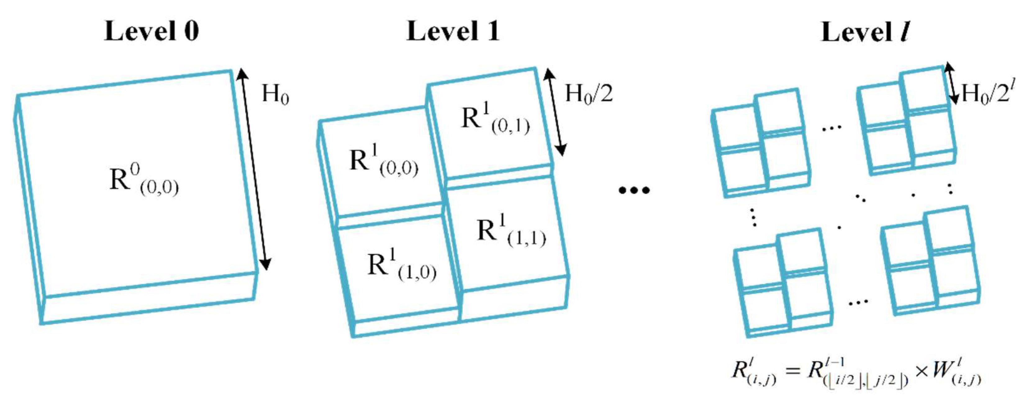
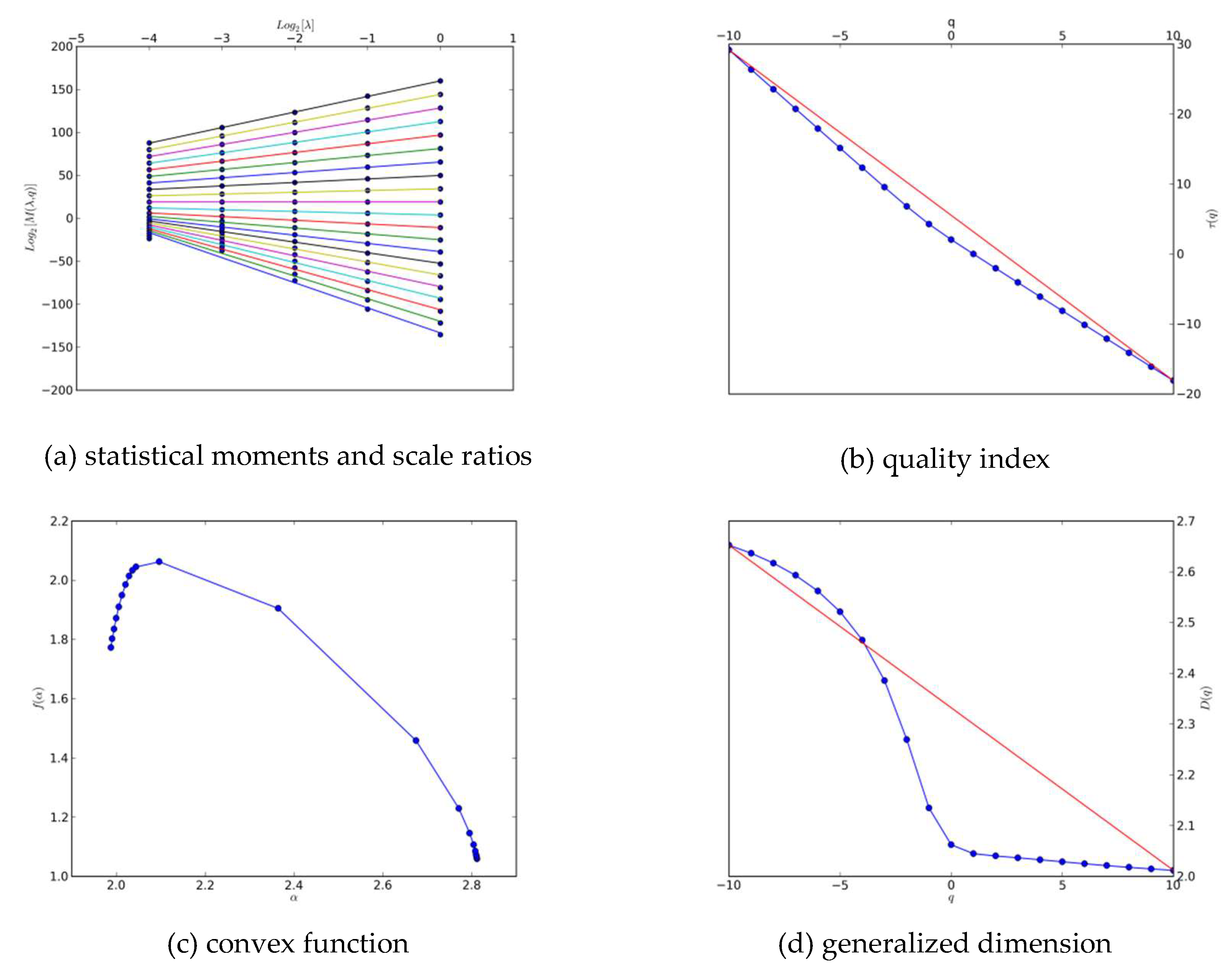
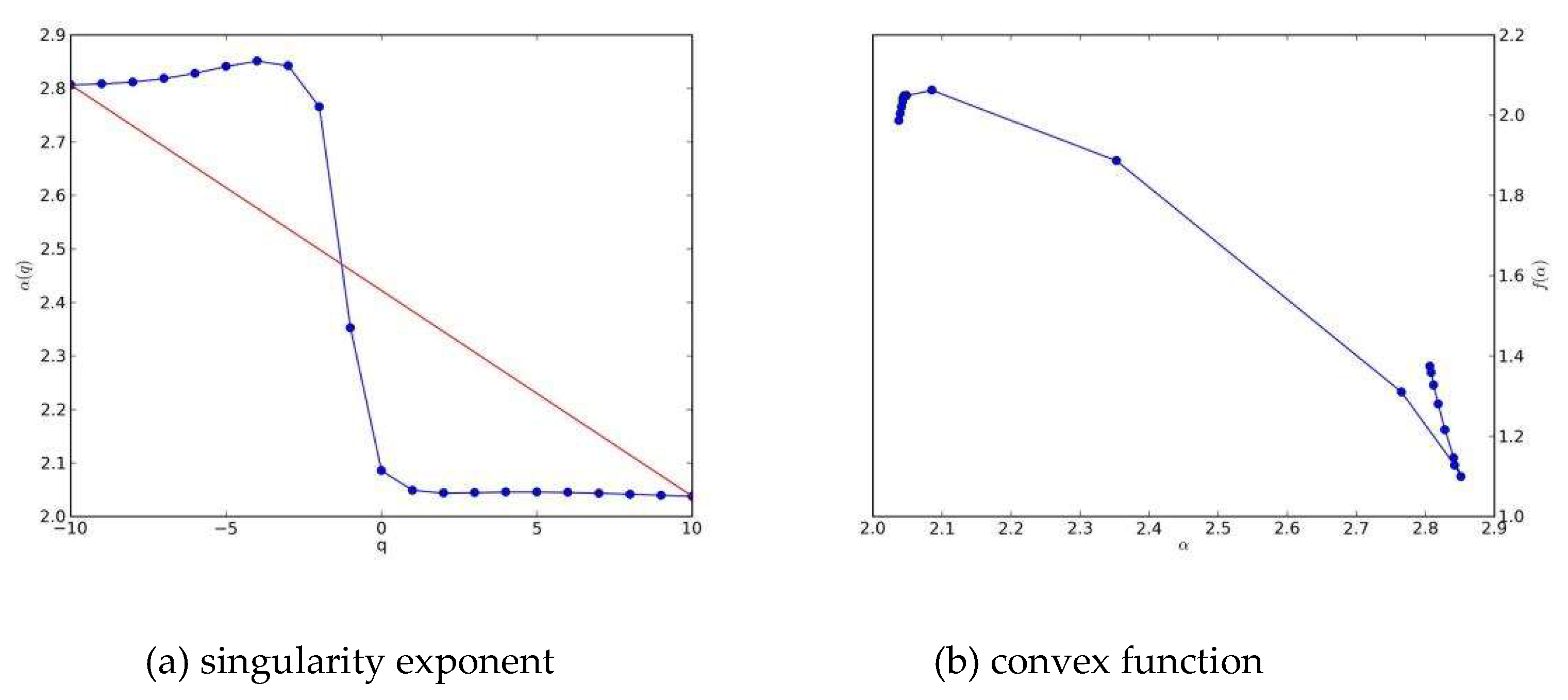
2.1.2. Multifractal Random Cascade (MFRC) Model

The multifractal analysis is a quantitative tool to describe the mass distribution of fractal space. Many researchers have proposed the self-similarity-based spatial downscaling method by utilizing the multifractal characteristics of precipitation [38,39]. The MFRC model employed in this study was derived from Pathirana and Herath’s work [39], and the random cascade process is depicted in Figure 1.

The homogeneous multifractal precipitation is expressed by the following equation:

$$M_{\left(i,j\right)}^l=\{\begin{array}{l}{M}_{\left(⎣i/2⎦,⎣j/2⎦\right)}^{l-1}\times W_{\left(i,j\right)} , l > 0\\ M_{\left(i,j\right)}^0\hspace{1em}\hspace{1em}\hspace{1em}\hspace{1em} , l=0\end{array}$$

(10)

where $i/j$ denotes the row/column index in the grid, and $W_{\left(i,j\right)}$ represents the random cascade weight in cell ($i,j$) to obtain level l homogeneous precipitation $M_{\left(i,j\right)}^l$. In this work, $M_{\left(i,j\right)}^0$ denotes the level 0 homogeneous field, while the initial 10 km precipitation data, which covers the entire study region as an 85 × 56 grid, is the 4th level field $(M_{\left(i,j\right)}^4$).

The $W_{\left(i,j\right)}$ in Equation (10) influences the downscaling results directly, and it can be calculated by Equations (11)–(13):

$$W_{\left(i,j\right)}=B{Y}_{\left(i,j\right)}$$

(11)

$$P\left[B=0\right]=1-b^{-\beta },P\left[B=b^{\beta }\right]=b^{-\beta }$$

(12)

$$Y_{\left(i,j\right)}=b^{-{\sigma }^2\frac{lnb}{2}+\sigma X_{\left(i,j\right)}}$$

(13)

where $b$ denotes the branching number with value of 4, $\beta$ and $\sigma$ are parameters of the β-lognormal model, and $X_{\left(i,j\right)}$ represents the random variable following a standard normal distribution according to classical multifractal theory. Combining Equations (11)–(13) and the Mandelbrot–Kahane–Peyriere (MKP) equations [32,38,49], $W_{\left(i,j\right)}$ yields Equations (14)–(19):

$$P\left[W_{\left(i,j\right)}=0\right]=1-b^{-\beta }$$

(14)

$$P\left[W_{\left(i,j\right)}{=b}^{\beta -{\sigma }^2\frac{lnb}{2}+\sigma X_{\left(i,j\right)}}\right]=b^{-\beta }$$

(15)

$$\beta =1+\frac{\tau \prime \left(q\right)}{2}-\frac{\tau ″\left(q\right)}{2}q+\frac{\tau ″\left(q\right)}{4}$$

(16)

$$k=\frac{\tau ″\left(q\right)}{2lnb}$$

(17)

$$\tau \left(q\right)=\underset{l\to \infty }{\lim }\frac{{log}_2{Q}^l\left(q\right)}{-{log}_2{\lambda }_l}$$

(18)

$${\lambda }_l=b^{-l/2},l=0,1,2,\dots .$$

(19)

where ${\lambda }_l$ represents the level l scale ratio, $Q^l\left(q\right)$ denotes the qth order statistical moment of $M_{\left(i,j\right)}^l$, and $q$ is in the range [−10, 10] in this study; $\tau \left(q\right)$ is the quality index describing the fractal characteristic of precipitation, while ${\tau }^{\prime }\left(q\right)$ and $\tau ″\left(q\right)$ are the first and second derivatives of $\tau \left(q\right)$, respectively.

In the estimation of β and $k$ and the subsequent downscaling process, it is necessary to recover the spatial heterogeneity of the estimated precipitation in the end, and this can be achieved by Equation (20) as follows:

$$R_{\left(i,j\right)}^l=M_{\left(i,j\right)}^l·G_{\left(i,j\right)}^l$$

(20)

where $R_{\left(i,j\right)}^l$/$G_{\left(i,j\right)}^l$ denotes the value of the l-th level estimated/heterogeneous precipitation in cell (i,j). The level-4 heterogeneous precipitation at the 10 km scale is calculated by Equation (21):

$$G_{\left(i,j\right)}^4=N^4\times \frac{A_{(i,j)}}{{{\displaystyle \sum }}_{i,j}{A}_{(i,j)}}$$

(21)

where $A_{(i,j)}$ denotes the monthly average precipitation value in cell (i,j) in a specific month during the study period, and $N^4$ represents the total number of level 4 grid cells.

From Equations (20) and (21), it is possible to calculate $M_{\left(i,j\right)}^4$ from 10 km satellite precipitation data. The expected value of $W_{\left(i,j\right)}$ equals 1; therefore, $M_{\left(i,j\right)}^0$ equals the average of $M_{\left(i,j\right)}^4$. Then it is possible to obtain the model parameters $\beta$ and $\sigma$ from Equations (16) and (17) with which to calculate the higher resolution homogeneous precipitation ($M_{\left(i,j\right)}^l$).

The recovery of level-l precipitation heterogeneity is achieved with Equation (22) (Posadas et al. 2015):

$$R_{\left(i,j\right)}^l=T_{\left(i,j\right)}^l\times \frac{M_{\left(i,j\right)}^l{G}_{\left(i,j\right)}^l}{{{\displaystyle \sum }}_{i,j}{M}_{\left(i,j\right)}^l{G}_{\left(i,j\right)}^l}$$

(22)

where $T^l$ denotes the large-scale forcing factor, and $G_{\left(i,j\right)}^l$ and $T_{\left(i,j\right)}^l$ can be calculated with Equation (23):

$$G_{\left(i,j\right)}^l=G_{\left(\overline{i},\overline{j}\right)}^4 , T_{\left(i,j\right)}{}^l=N^l\times R_{\left(\overline{i},\overline{j}\right)}^4 \overline{i}=⎣i/2^{l-4}⎦,\overline{j}=⎣j/2^{l-4}⎦$$

(23)

The initial 10 km precipitation field was downscaled to 0.625 km at the 8th level in this study to enhance the heterogeneity of the precipitation; the model always runs the random cascade process for multiple times and takes the mean value of different results. Finally, the 1 km high-resolution precipitation estimates were obtained by bilinear interpolation from the average downscaled field.

2.1.3. GWR-MF Model

The GWR-MF model uses the MFRC model to downscale the regression residual of the point set in the study area obtained by the GWR model to obtain the residual after downscaling, and then adds the residual of the point set obtained with the corresponding point data of GWR to compensate and correct the results after downscaling of the GWR.

The results of the GWR-MF model are obtained by MFRC interpolation based on GWR, and its principle can be expressed as follows:

R_GWR-MF = R_GWR + Residual_MF

(24)

where GWR-MF is the precipitation prediction value, R_GWR is the GWR precipitation after downscaling, and Residual_MF is the residual value after downscaling of the MFRC model.

The MFRC model requires the l-th heterogeneous precipitation to recover heterogeneity. The GWR-MF model applies GWR to obtain high-resolution monthly precipitation which can be used to enhance the heterogeneity of high-resolution daily precipitation. In this study, GWR high-resolution (1 km × 1 km) monthly precipitation with spatial resolution of 1 km was introduced to restore the heterogeneity of MFRC model. Recall that in Equation (22) that $G_{\left(i,j\right)}^l$ denotes the value of the l-th level heterogeneous precipitation in cell (i,j), and it equals the average monthly precipitation downscaled with the GWR at a 1 km × 1 km spatial resolution.

2.1.4. Validation

This paper adopts the correlation coefficients (CCs) and relative bias (bias) to measure the accuracy of the predicted precipitation. A CC close to 1 (or 0) indicates a strong positive statistical relation (or no statistical relation) between the predicted precipitation and the ground observations. The absolute value of bias close to zero is desirable from the perspective of calculating predictions nearly identical to observations. These evaluation criteria are given by the following equations:

$$CC=\frac{{{\displaystyle \sum }}_{i=1}^n(D_i-\overline{D}){(E_i-\overline{E})}^2}{{{\displaystyle \sum }}_{i=1}^n{(D_i-\overline{D})}^2{{\displaystyle \sum }}_{i=1}^n{(E_i-\overline{E})}^2}$$

(25)

$$Bias=\frac{{{\displaystyle \sum }}_{i=1}^n{E}_i}{{{\displaystyle \sum }}_{i=1}^n{D}_i}-1$$

(26)

where $D_i$ and $E_i$ denote gauge-measured precipitation and the final downscaled estimates, respectively, while $\overline{D}$ and $\overline{E}$ represent the average values of $D_i$ and $E_i$, respectively.

The performance of the GWR model is quantified by the goodness of fit (R²), the standardized residuals (StdResid), and the AICc value, in which R², and StdResid can be calculated with the initial precipitation field and the predicted value at coarse resolution; and the AICc value is computed by Equation (9) for the GWR model. R² ranges between 0 and 1 for positively correlated variables, and the larger it is, the stronger the statistical relation between predictions and observations. The magnitude and distribution of StdResid can reflect the model’s robustness and fitness to some extent. The more significant the multifractal characteristics in the initial satellite-based precipitation field are, the more reliable the MFRC downscaled results are in theory. In the end, 1 km downscaled precipitation should be as smooth as possible to reveal the natural rainfall phenomenon.

2.2. Study Area and Data

2.2.1. Study Areas

Hubei Province (29˚1′–33˚6′ N, 108˚21′–116˚7′ E), which is located in Central China, with an area of approximately 185,900 km², was selected as a case study area in this study and is shown in Figure 2. The study region has a complex landform, and the topography is slanted downward form east to west. The Yangtze River and its longest tributary, the Han River, cross the province, and thousands of lakes dot the landscape of Jianghan Plain, giving Hubei the name of the “Province of Lakes”. The Jianghan Plain occupies most of Central and Southern Hubei, while the west and the peripheries are more mountainous, with ranges such as the Wudang Mountains and the Daba Mountains. Hubei Province has a humid subtropical climate, with four distinct seasons. Precipitation shows great spatial variation due to geography and the climate, and the overall trends of precipitation decrease from the southeast to the northwest.

2.2.2. Precipitation Datasets

The GPM aims to provide a new generation of global rainfall and snowfall observations, as a successor of the TRMM. The Core Observatory satellite was launched in February 2014 by the National Aeronautics and Space Administration (NASA, Washington, D.C., United States) and the Japan Aerospace and Exploration Agency (JAXA, Tokyo, Japan), carrying the GPM Microwave Imager (GMI) and the Dual-Frequency Precipitation Radar (DPR). The GPM sensors improve the ability to detect solid precipitation due to the new high-frequency channels (165.6 and 183.3 GHz) for the GMI and Ka-band (35.5 GHz) for the DPR. The most advanced IMERG is a 0.5 h, 0.1° × 0.1° resolution, 60° N–60° S spatial coverage dataset and is computed by using GPM and several other satellite precipitation products, using the Goddard Profiling Algorithm (GPROF). Three modes (early, late, and final runs) are available with the IMERG product depending on latency and requirements, and the final-run IMERG product can provide more accurate results based on monthly rain gauge calibration. The latest level-3 05b version of IMERG final-run monthly estimates from 2015 to 2017 selected in this study was downloaded from https://pmm.nasa.gov/data-access/downloads/gpm (Accessed on 16 June 2021). All raw data are clipped to the study area, reprojected to the UTM 49N, and resembled 10 km resolutions as initially coarse precipitation fields, which still hold the same accuracy as the original 0.1° IMERG product in geographic coordinate systems.

The ground-observed precipitation of 75 rain gauge stations was parsed from the Hubei Meteorological Bureau website (http://www.hbqx.gov.cn/qx_tqsk.action, accessed on 20 January 2021), as shown in Figure 2. The stations are distributed randomly over the entire study area. Since the function of rain-gauge data was to validate the downscaling results independently, they were not used to correct GPM/IMERG precipitation.

The correlation between the original GPM and the site data is shown in Figure 3. Most of the results are above 0.6, which indicates a clear correlation between the two. Therefore, this paper uses the precipitation of 75 rain gauges to verify the downscaling results.

2.2.3. DEM and LST Datasets

DEM and LST data were extensively used as explanatory variables in spatial downscaling research for satellite-based precipitation. The 30 m ASTER GDEM (V2) data were selected in this paper and downloaded from the Geospatial Data Cloud (http://www.gscloud.cn) (Accessed on 16 June 2021). Terra-MODIS daytime LST products (MOD11A2) with 1 km resolution used in the study were obtained from the NASA Land Processes Distributed Active Archive Center (LP DAAC, https://ladsweb.modaps.eosdis.nasa.gov) (Accessed on 16 June 2021). The monthly LST data were generated by averaging four 8-day MOD11A2 data files for each calendar month, and the missing values were interpolated by the nearest neighbor resampling algorithm. Both DEM and LST data were adjusted to the same spatial range and projection as the processed GPM/IMERG precipitation fields, and then resembled and aggregated to 10 km and 1 km resolutions. The longitude and latitude information was ultimately calculated from the projected raster.

3. Results

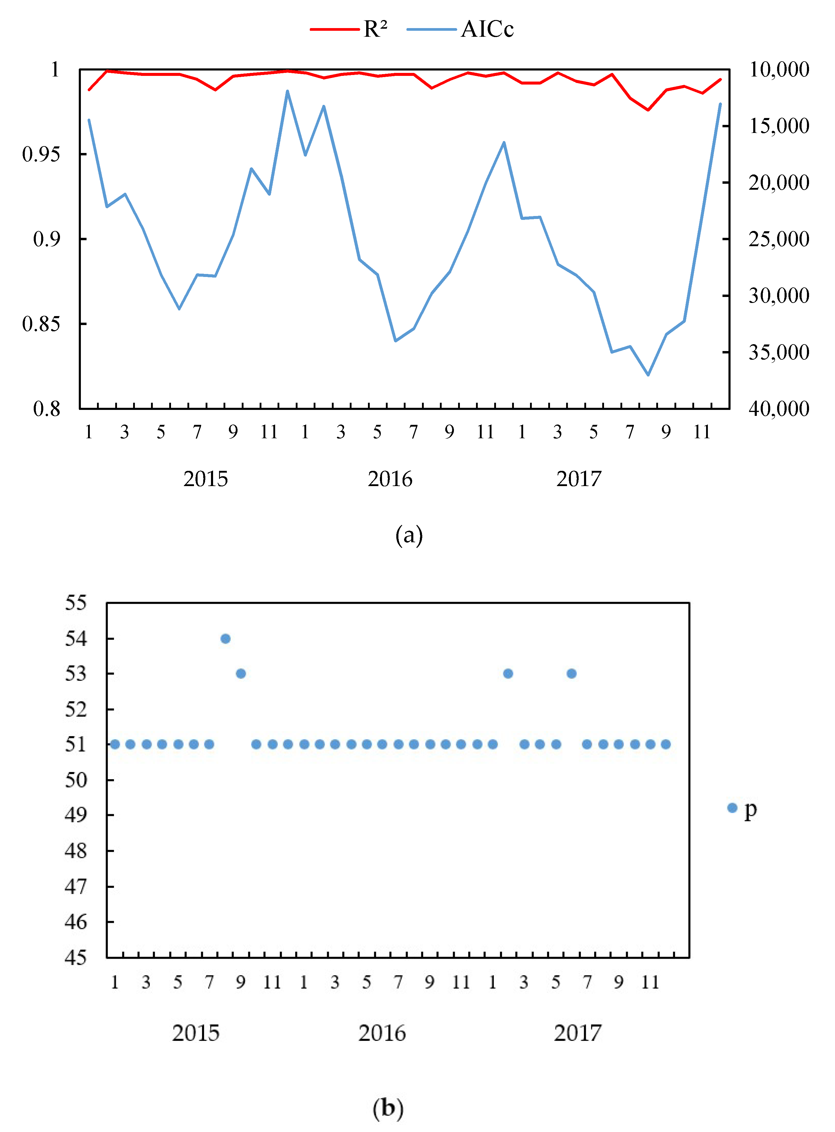
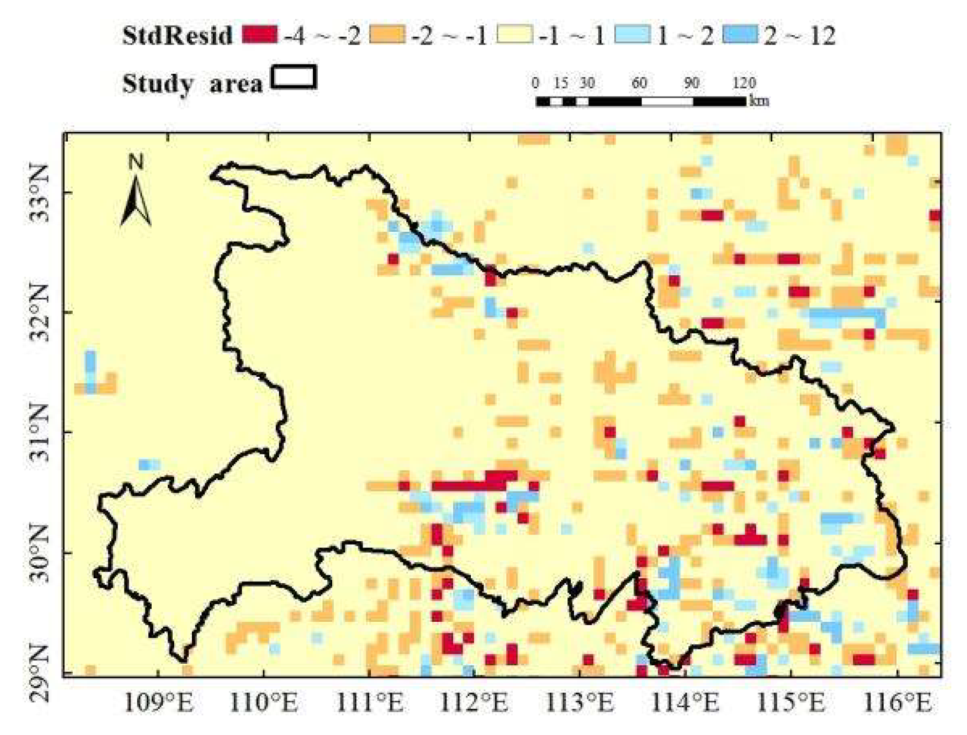
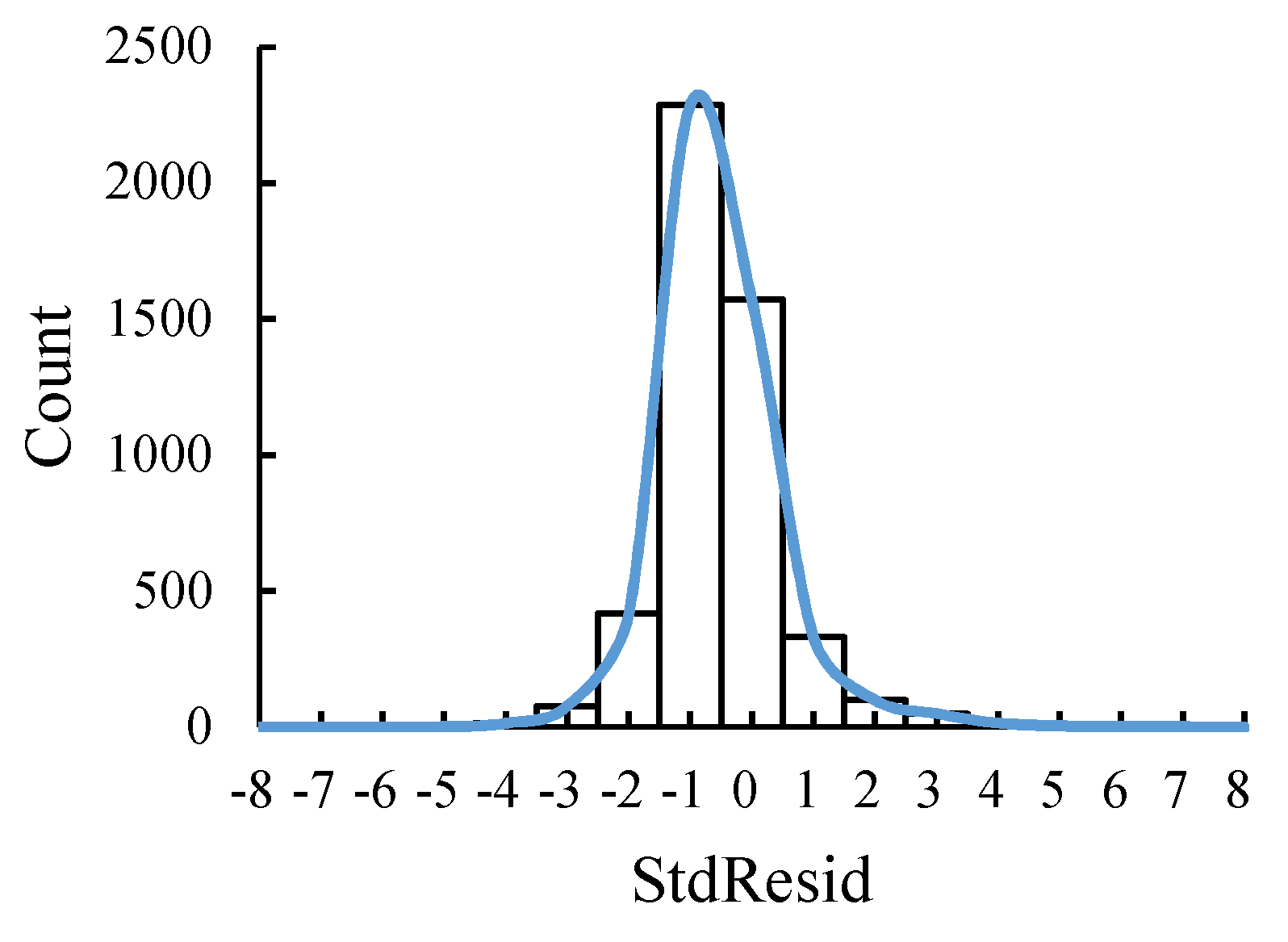
3.1. The Performances of GWR Models

The GWR models adopting the adaptive bi-square kernel function were constructed in this paper for all 36 months, and the optimal p-value [50], which represents the number of neighbors counted in the prediction of the current position, mostly determines the GWR model’s performance. The R² and AICc of 36 GWR models are shown in Figure 4a, and the p-values are shown in Figure 4b.

The AICc value of the GWR model depends on the $SSE$ value (see Equation (9)). The average AICc value during the whole study period was 25,108.379. At the same time, due to the obvious influence of different months, the AICc value fluctuates seasonally.

The p-values of 36 GWR models are in the range of 51–54, irregularly, as shown in Figure 4b, which indicates that tens of neighbor points were counted into the local regression at the current position. The non-stationarity in the neighborhood within approximately 50–60 km is slight enough to ignore it and can reasonably achieve the local linear regression. Residuals in GWR models were not required to be normally distributed, because the WLS is a biased estimation method from the beginning. For the same month in December 2016, the StdResid values and the distribution curve of the GWR model are depicted in Figure 5 and Figure 6. There are no severe clusters in the whole study area, and the StdResid values are mainly in the range of −2~2.

3.2. The Performances of MFRC Models

A scale region that obeys the power law is called non-scaling, which is a requirement of fractal analysis, in which case the relationships between the statistical moments, $Q\left(\lambda ,q\right)$, and the scale ratios, $\lambda$, appear as straight lines in a log–log diagram. According to multifractal theory [7,32,37,39] there are four phenomena that can indicate a certain object possessing multifractal characteristics, which can be described as follows: the quality index, $\tau \left(q\right)$, is not a simple linear function of the order q of $Q\left(\lambda ,q\right)$; the singularity exponent, $\alpha \left(q\right)$, is strictly decreasing with the increment of q; the multifractal spectrum, $f\left(\alpha \right)$, is a convex function of $\alpha$ which reaches the single peak when $\alpha \left(q\right)=0$; and the generalized dimension, $D\left(q\right)$, decreases monotonically with the increment of q.

The large majority of the 36 monthly homogenized precipitation fields during the study period have been proven to be multifractal objects, and the indicators mentioned above in July 2016, the same month analyzed in the GWR model, are depicted in Figure 7, and they reveal the typical multifractal characteristics. However, aberrations at different degrees also occurred in homogenized precipitation in February and December 2015, November 2016, and December 2017. Figure 8 illustrates the anomalies present in the homogenized precipitation field in February 2015.

All downscaling methods were designed to enhance the heterogeneity of precipitation fields at a subpixel level in practice—in other words, to create reasonable and diverse precipitation intensity values within a 100 km² area—since the initial spatial resolution is 10 km. For the MFRC downscaling model, the sub-pixel heterogeneity is solely produced by the random variable X of the cascade generator, in that it always takes the mean values of multiple downscaled results because of the absolute randomness at any position.

Unfortunately, a kind of self-contradiction that creates heterogeneity with X and averages the different results, so the number of times the cascade process is run is essential for the performance of the final model and the consumption of computing resources. Twenty times was determined to be feasible in this work based on abundant experiments, and the initial 10 km precipitation grid and the downscaled results of running the cascade process for 10/20/50 times in December 2015 are displayed in Figure 9. Many tiny spots with errors exist in the “10 times” downscaled results and those errors are visibly reduced in the “20 times” downscaled results, whose value range is closer to the initial field as well. The “50 times” downscaled results do not show significant improvements compared to the “20 times” results, and instead, considerable time is wasted in processing.

3.3. The Performances of GWR-MF Models

The Multifractal objects usually have a self-similarity. Therefore, the downscaling decomposition process of the precipitation field in the random cascade model requires the precipitation field to have statistical homogeneity in order to reflect the regional self-similarity of the homogeneous background field.

In the downscaling process of the MFRC model, with the help of the GPM monthly mean of precipitation field, to restore the heterogeneity of the precipitation field, the downscaling results show obvious mosaic characteristics. To explore whether the use of the low-resolution heterogeneous precipitation field in the process of restoring the spatial heterogeneity of the high-resolution precipitation background field has an impact on the downscaling results, this paper uses the corresponding monthly scale precipitation field with 1 km resolution obtained by the GWR model to enhance the spatial heterogeneity of the MFRC model after downscaling. The local regression is well realized by using the downscaling results of the GWR model with a 1 km resolution to enhance heterogeneity. As seen from Figure 10, the downscaling result of the MFRC model has no obvious mosaic characteristics or clustering phenomenon.

Table 1. Results of 36 months accuracy evaluation of the GWR-MF model.

Month	2015		2016		2017
	CC	Bias	CC	Bias	CC	Bias
1	0.549	0.080	0.806	0.442	0.807	0.315
2	0.964	0.056	0.772	0.008	0.651	0.338
3	0.766	0.172	0.831	0.061	0.917	0.009
4	0.887	0.056	0.891	−0.002	0.794	−0.011
5	0.801	0.125	0.703	0.222	0.698	0.155
6	0.843	0.004	0.798	0.186	0.890	0.193
7	0.791	0.114	0.783	−0.125	0.689	0.207
8	0.273	0.060	0.431	−0.030	0.828	−0.015
9	0.773	0.114	0.832	0.142	0.782	−0.032
10	0.787	0.024	0.463	0.105	0.874	0.023
11	0.780	0.177	0.738	0.128	0.824	0.158
12	0.856	0.402	0.893	0.210	0.841	0.547

shows the 36-month downscaling accuracy evaluation results based on the GWR-MF model.

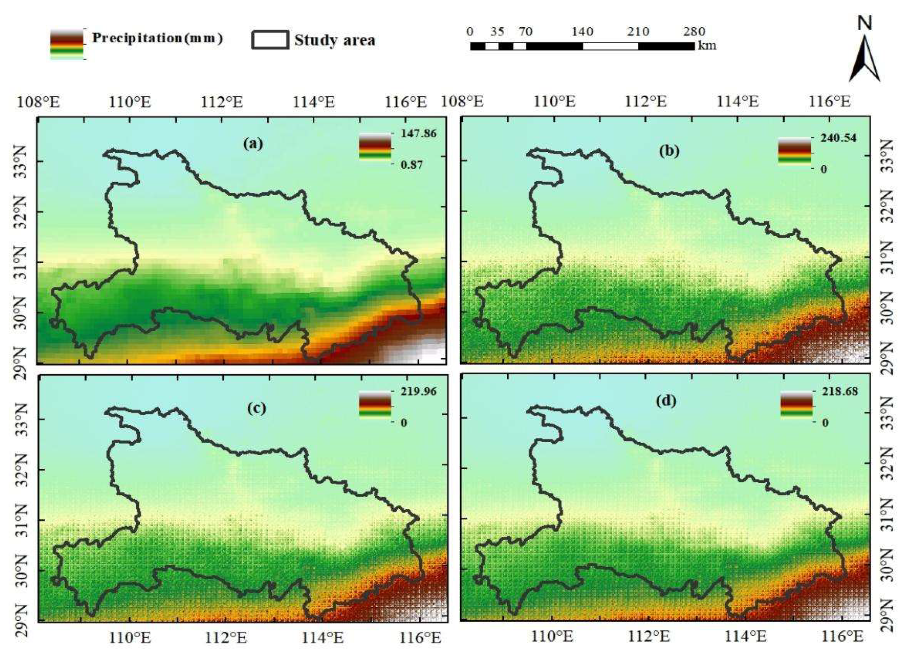
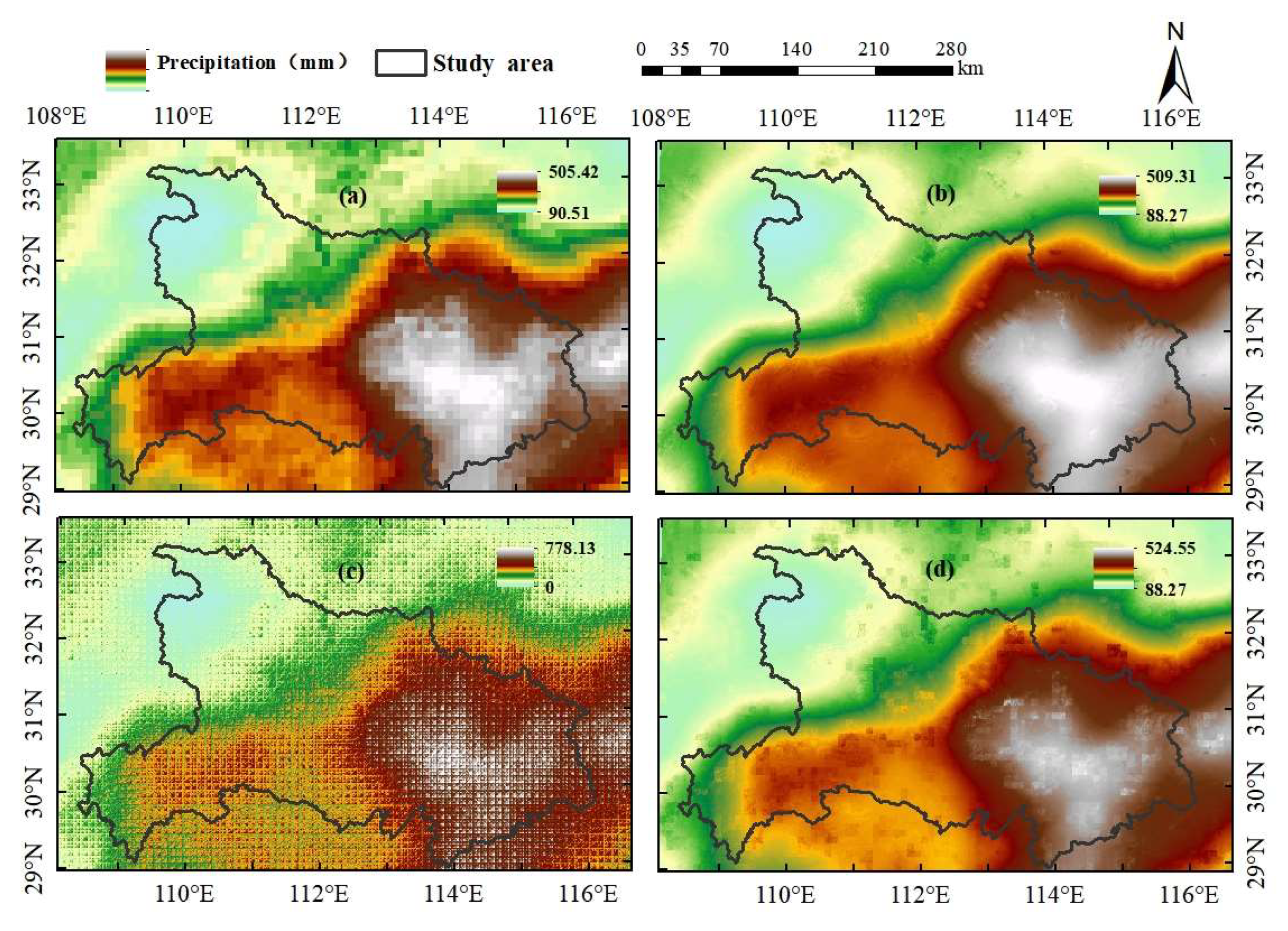
3.4. Comparison of 1 km Final Downscaled Results of GWR, MFRC, and GWR-MF Models

Ignoring the anomalies for specific months in GWR and MFRC models construction, we see that all 36 monthly precipitation fields derived from the GPM/IMERG products were downscaled from 10 km spatial resolution to 1 km in this study. The accuracy assessment was accomplished with CC and bias by utilizing the initial 10 km precipitation data. The downscaled results of the three methods and the ground-observed precipitation at 75 rain gauge stations were analyzed.

As depicted in Figure 11, satellite-derived 10 km precipitation data possess the equivalent accuracy and quality relative to the rain gauges’ observations at monthly temporal scale, which holds a mean CC value of 0.770 and a mean bias value of 13.202% for the entire study period. The largest CC value of 0.966 shows up in February 2015, and it is a little overestimated in satellite precipitation fields for most months; however, the discrepancy between the two datasets may also be quite huge under extreme situations. Calibration of initial precipitation fields, not discussed in this study, is necessary for better downscaling performance due to the ineluctable random errors to some extent.

Compared to the GPM/IMERG-based 10 km precipitation fields, the downscaled results of the GWR and MFRC models can remain with the same accuracy as the mean CC values of the GWR/MFRC models, which are 0.771 and 0.731, respectively, and the mean Bias values of the GWR/MFRC models are 14.018% and 11.865%, respectively, where the data points and lines are severely overlapped in Figure 11.

The results show that the three adopted downscaling methods for the monthly 10 km resolution satellite precipitation cannot significantly enhance the sub-pixel heterogeneity according to the similar statistical index (CC/Bias), even in the GWR/MFRC results. Perhaps the predicted precipitation should have been as smooth as possible and identical to the original 10 km data to maintain the intrinsic details and consistency. The downscaling goal was already successfully satisfied when the high-resolution estimated precipitation quality did not decrease obviously, and the spatial distribution was not distorted in the whole study area.

Based on an analysis of the downscaling accuracy evaluation results of the GWR/MFRC model, the downscaling results of the GWR model have a higher correlation with the true value of precipitation, but in terms of bias evaluation, the MFRC model is better than the GWR model. Combining the GWR model with MFRC for hybrid downscaling can maintain and improve the correlation and reduce the deviation of the results.

Since the GWR downscaling model in July 2016 holds a high goodness of fit (R² = 0.989), and the multifractal characteristics are also satisfactory in the same month, the initial 10 km precipitation grid and the downscaled results of the three models in July 2016 are displayed in Figure 12, and the CC and bias values of the four fields are compared in

Table 2. CC and bias values of four precipitation grids in July 2016.

Index	10 km	GWR	MFRC	GWR-MF
CC	0.771	0.775	0.753	0.783
Bias	−13.7%	−13.3%	−15.2%	−12.5%

.

The scatter diagram of precipitation field data and station observation data after downscaling in July 2016 is shown in Figure 13. The downscaling data of the GWR model and MF model are very close to GPM product data, and the downscaling data of the MFRC model are quite different from the GPM product data in some months. The accuracy of downscaling data of several models is reduced in meteorological stations with large precipitation, and the data of GPM data are significantly different in meteorological stations with large precipitation.

The GWR/MFRC downscaled results have a good performance, with a substantial distribution and a rational value range. The difference between the GWR and MFRC results is that the former is smoother, and the latter shows an apparent mosaic-like trait suggesting that the spatial resolution did not improve. The downscaling results of the GWR-MF model have higher CC/lower bias values than the GWR/MFRC model.

The horizontal and vertical profiles of the GWR and MFRC downscaled results in July 2016 at the Wuhan rain gauge station (114.05° E, 30.6° N) are depicted in Figure 14. Both profile curves of the MFRC results have many jaggies corresponding to the mosaics above and the curves of the GWR results are much smoother. As discussed in the analysis of MFRC models construction (see Section 3.2), in some instances, the prediction is too random and produces unavoidable errors in an original 10 km pixel due to the internal defect of the classic MRFC method that brings the mosaics or jaggies into the final results. Although not all downscaled results have been displayed or analyzed in diagrams one by one, there is sufficient evidence to conclude that the GWR models are more reliable and suitable than the MRFC models for spatial downscaling of the latest monthly GPM/IMERG precipitation products.

4. Discussion

The improved CC of the GWR model accounts for 47.2% of the model improvement, and the bias-accuracy improvement accounts for 50%. The GWR model needs different influence factors for correlation analysis besides latitude and longitude. Different influencing factors lead to diverse effects on downscaling, the overall improvement in accuracy is uncertain, so it needs further exploration.

The MFRC interpolation is not smooth enough, and it is hard to avoid a lot of mosaics. Meanwhile, there are many random errors, since not all of the months satisfied the prerequisite for the multifractal theory.

According to the obtained downscaling accuracy evaluation results, the spatial distribution of the precipitation background field after the downscaling of the GWR-MF model is the same as that of the MFRC model and initial precipitation background field, which shows that this method of downscaling of precipitation by the GWR-MF model is feasible.

When the rainfall value is large, the downscaling advantage of the GWR-MF model is more obvious than that of the GWR model and MFRC model. The introduction of the MFRC model is reasonable to improve the interpolation accuracy. The fusion of the GWR model and the MFRC model can improve the correlation coefficient and reduce the deviation.

In this paper, one of the reasons for the unsatisfactory results of the downscaling of the MFRC model is that the low-resolution heterogeneous precipitation field is still used in the process of restoring the spatial heterogeneity of the high-resolution precipitation background field. Based on the MFRC model and GWR model, the GWR-MF model is obtained to eliminate the influence of the low resolution heterogeneous precipitation field.

In the months with precipitation greater than 100 mm, the CC accuracy of the GWR-MF model improves by 11.1%, and bias-accuracy improves by 2.8% over the GWR model. Compared to the MFRC model, the CC accuracy of the GWR-MF model improves by 25% over the MFRC model, and the bias-accuracy improves by 25% over the GWR model. However, in the months with low rainfall, the accuracy of the GWR-MF model is still higher than the MFRC model, despite being lower than the GWR model. According to the statistical results from 2015 to 2017, the GWR-MF model performed well when the rainfall was relatively high. However, the conclusions still need to be confirmed by more data.

5. Conclusions

This paper investigated and evaluated the spatial downscaling performances and suitability of a typical GWR regression method, a multifractal-based weather generator (MFRC) and a hybrid downscaling method for the latest monthly GPM/IMERG precipitation products from 0.1° × 0.1° to 1 km × 1 km for the 2015 to 2017 period in Hubei Province, China. The main conclusions are as follows:

(1)

The original GPM product can accurately express the precipitation in the study area, which highly correlates with the site data from 2015 to 2017 (R² = 0.79) and overall presents the phenomenon of overestimation.

(2)

Based on the analyses of models construction and the accuracy assessment results, the GWR models are more reliable and suitable than the MRFC model, as they can perfectly maintain the equivalent accuracy relative to the initial precipitation fields and keep enough smoothness and consistency at a 1 km scale, as well.

(3)

The GWR-MF model can improve CC and bias to a certain extent. In the months with large precipitation in the study area, the superiority of the GWR-MF model is more obvious. The GWR-MF model can weaken a large number of mosaics in the downscaling of the MFRC model and avoid the disadvantage that the MFRC model cannot be established effectively in a few months during the study period.

The analyses and conclusions in this paper can offer a meaningful information for similar studies. The proposed model provides 1 km high-resolution data support for regional ecology, hydrology, agriculture, or other relevant applications. It is noteworthy that the discrepancy between the GPM/IMERG satellite products and the observed precipitation by rain gauges exists and visible in any time period, and the calibration of the GPM/IMERG series precipitation fields remains in progress.

The introduction of the GWR-MF model is reasonable in improving the interpolation accuracy, but the accuracy is lower than that of the GWR model in individual months. Since the experiments are only for precipitation over 36 months, it is necessary to confirm the universality of several downscaling models in the long time-series model in the future.

References

1. Duan, Z.; Liu, J.; Tuo, Y.; Chiogna, G.; Disse, M. Evaluation of eight high spatial resolution gridded precipitation products in Adige Basin (Italy) at multiple temporal and spatial scales. Sci. Total Environ. 2016, 573, 1536–1553. [Google Scholar] [CrossRef] [PubMed] [Green Version]
2. Tang, G.; Ma, Y.; Long, D.; Zhong, L.; Hong, Y. Evaluation of GPM Day-1 IMERG and TMPA Version-7 legacy products over Mainland China at multiple spatiotemporal scales. J. Hydrol. 2016, 533, 152–167. [Google Scholar] [CrossRef]
3. Yu, C.; Hu, D.; Liu, M.; Wang, S.; Di, Y. Spatio-temporal accuracy evaluation of three high-resolution satellite precipitation products in China area. Atmos. Res. 2020, 241, 104952. [Google Scholar] [CrossRef]
4. Xie, P.P.; Xiong, A.Y. A conceptual model for constructing high-resolution gauge-satellite merged precipitation analyses. J. Geophys. Res. Atmos. 2011, 116. [Google Scholar] [CrossRef]
5. Cecinati, F.; Rico-Ramirez, M.A.; Heuvelink, G.B.; Han, D. Representing radar rainfall uncertainty with ensembles based on a time-variant geostatistical error modelling approach. J. Hydrol. 2017, 548, 391–405. [Google Scholar] [CrossRef] [Green Version]
6. Liu, J.; Zhang, W.; Nie, N. Spatial downscaling of TRMM precipitation data using an optimal subset regression model with NDVI and terrain factors in the Yarlung Zangbo River Basin, China. Adv. Meteorol. 2018, 2018, 3491960. [Google Scholar] [CrossRef]
7. Huffman, G.J.; Adler, R.F.; Bolvin, D.T.; Gu, G.J.; Nelkin, E.J.; Bowman, K.P.; Hong, Y.; Stocker, E.F.; Wolff, D.B. The TRMM multisatellite precipitation analysis (TMPA): Quasi-global, multiyear, combined-sensor precipitation estimates at fine scales. J. Hydrometeorol. 2007, 8, 38–55. [Google Scholar] [CrossRef]
8. Huffman, G.J.; Bolvin, D.T.; Braithwaite, D.; Hsu, K.; Kidd, C.; Nelkin, E.J.; Sorooshian, S.; Tan, J.; Xie, P. NASA Global Precipitation Measurement (GPM) Integrated Multi-satellitE Retrievals for GPM (IMERG). Available online: https://gpm.nasa.gov/sites/default/files/document_files/IMERG_ATBD_V06.pdf (accessed on 11 June 2021).
9. Huffman, G.J. The Transition in Multi-Satellite Products from TRMM to GPM (TMPA to IMERG). Available online: https://gpm.nasa.gov/sites/default/files/2020-10/TMPA-to-IMERG_transition_201002.pdf (accessed on 11 June 2021).
10. Bi, E.G.; Gachon, P.; Vrac, M.; Monette, F. Which downscaled rainfall data for climate change impact studies in urban areas? Review of current approaches and trends. Theor. Appl. Climatol. 2015, 127, 685–699. [Google Scholar] [CrossRef]
11. Asong, Z.E.; Khaliq, M.N.; Wheater, H.S. Projected changes in precipitation and temperature over the Canadian Prairie Provinces using the Generalized Linear Model statistical downscaling approach. J. Hydrol. 2016, 539, 429–446. [Google Scholar] [CrossRef]
12. Manzanas, R.; Gutiérrez, J.M.; Fernández, J.; Van Meijgaard, E.; Calmanti, S.; Magariño, M.E.; Cofiño, A.S.; Herrera, S. Dynamical and statistical downscaling of seasonal temperature forecasts in Europe: Added value for user applications. Clim. Serv. 2018, 9, 44–56. [Google Scholar] [CrossRef]
13. Jing, W.; Yang, Y.; Yue, X.; Zhao, X. A comparison of different regression algorithms for downscaling monthly satellite-based precipitation over north China. Remote Sens. 2016, 8, 835. [Google Scholar] [CrossRef] [Green Version]
14. Baghanam, A.H.; Eslahi, M.; Sheikhbabaei, A.; Seifi, A.J. Assessing the impact of climate change over the northwest of Iran: An overview of statistical downscaling methods. Theor. Appl. Climatol. 2020, 141, 1135–1150. [Google Scholar] [CrossRef]
15. Cai, M.; Lv, Y.; Yang, S.; Zhou, Q. TRMM precipitation downscaling in the data scarce Yarlung Zangbo River basin. J. Beijing Norm. Univ. Nat. Sci. 2017, 53, 111–119. [Google Scholar]
16. Duan, Z.; Bastiaanssen, W.G.M. First results from Version 7 TRMM 3B43 precipitation product in combination with a new downscaling–calibration procedure. Remote Sens. Environ. 2013, 131, 1–13. [Google Scholar] [CrossRef]
17. Ma, Z.Q.; Zhou, L.Q.; Yu, W.; Yang, Y.Y.; Teng, H.F.; Shi, Z. Improving TMPA 3B43 V7 data sets using land-surface characteristics and ground observations on the Qinghai–Tibet Plateau. IEEE Geosci. Remote Sens. Lett. 2018, 15, 178–182. [Google Scholar] [CrossRef]
18. Brunsdon, C.; Fotheringham, A.S.; Charlton, M.E. Geographically weighted regression: A method for exploring spatial nonstationarity. Geogr. Anal. 1996, 28, 281–298. [Google Scholar] [CrossRef]
19. Stewart Fotheringham, A.; Charlton, M.; Brunsdon, C. The geography of parameter space: An investigation of spatial non-stationarity. Int. J. Geogr. Inf. Syst. 1996, 10, 605–627. [Google Scholar] [CrossRef]
20. Chen, F.; Liu, Y.; Liu, Q.; Li, X. Spatial downscaling of TRMM 3B43 precipitation considering spatial heterogeneity. Int. J. Remote Sens. 2014, 35, 3074–3093. [Google Scholar] [CrossRef]
21. Zhan, C.; Han, J.; Hu, S.; Liu, L.; Dong, Y. Spatial downscaling of GPM annual and monthly precipitation using regression-based algorithms in a mountainous area. Adv. Meteorol. 2018, 2018, 1506017. [Google Scholar] [CrossRef] [Green Version]
22. Jaber, S.M. Comparative evaluation of statistically downscaling Tropical Rainfall Measuring Mission (TRMM) and Global Precipitation Measurement (GPM) mission precipitation data: Evidence from a typical semi-arid to arid environment. Spat. Inf. Res. 2021, 29, 331–338. [Google Scholar] [CrossRef]
23. Wang, M.; He, G.; Zhang, Z.; Wang, G.; Zhang, Z.; Cao, X.; Wu, Z.; Liu, X. Comparison of spatial interpolation and regression analysis models for an estimation of monthly near surface air temperature in China. Remote Sens. 2017, 9, 1278. [Google Scholar] [CrossRef] [Green Version]
24. Chen, C.; Zhao, S.; Duan, Z.; Qin, Z. An improved spatial downscaling procedure for TRMM 3B43 precipitation product using geographically weighted regression. IEEE J. Sel. Top. Appl. Earth Obs. Remote Sens. 2015, 8, 4592–4604. [Google Scholar] [CrossRef]
25. Xu, S.; Wu, C.; Wang, L.; Gonsamo, A.; Shen, Y.; Niu, Z. A new satellite-based monthly precipitation downscaling algorithm with non-stationary relationship between precipitation and land surface characteristics. Remote Sens. Environ. 2015, 162, 119–140. [Google Scholar] [CrossRef]
26. Zhang, Y.Y.; Li, Y.G.; Ji, X.; Luo, X.; Li, X. Fine-resolution precipitation mapping in a mountainous watershed: Geostatistical downscaling of TRMM products based on environmental variables. Remote Sens. 2018, 10, 119. [Google Scholar] [CrossRef] [Green Version]
27. Siabi, N.; Sanaeinejad, S.H.; Ghahraman, B. Comprehensive evaluation of a spatio-temporal gap filling algorithm: Using remotely sensed precipitation, LST and ET data. J. Environ. Manag. 2020, 261, 110228. [Google Scholar] [CrossRef]
28. Colditz, R.R.; Villanueva, V.L.A.; Tecuapetla-Gómez, I.; Mendoza, L.G. Temporal relationships between daily precipitation and NDVI time series in Mexico. In Proceedings of the 2017 9th International Workshop on the Analysis of Multitemporal Remote Sensing Images (MultiTemp), Brugge, Belgium, 27–29 June 2017; IEEE: Manhattan, NY, USA, 2017; pp. 1–4. [Google Scholar]
29. Xing, Z.; Ni, G.H.; Chen, S.; Sun, T. Remapping annual precipitation in mountainous areas based on vegetation patterns: A case study in the Nu River basin. Hydrol. Earth Syst. Sci. 2017, 21, 999–1015. [Google Scholar] [CrossRef] [Green Version]
30. Mandelbrot, B.B. Intermittent turbulence in self-similar cascades: Divergence of high moments and dimension of the carrier. J. Fluid Mech. 1974, 62, 331–358. [Google Scholar] [CrossRef]
31. Mandelbrot, B.B. Fractals: Form, Chance and Dimension; Translated from the French. Revised edition; W. H. Freeman and Co.: San Francisco, CA, USA, 1977. [Google Scholar]
32. Over, T.M.; Gupta, V.K. A space-time theory of mesoscale rainfall using random cascades. J. Geogr. Res. 1996, 101, 319–331. [Google Scholar] [CrossRef]
33. Schertzer, D.; Lovejoy, S. Physical modeling and analysis of rain and clouds by anisotropic scaling multiplicative processes. J. Geophys. Res. Atmos. 1987, 92, 9693–9714. [Google Scholar] [CrossRef]
34. Mandelbrot, B. How long is the coast of Britain? Statistical self-similarity and fractional dimension. Science 1967, 156, 636–638. [Google Scholar] [CrossRef] [Green Version]
35. Pathirana, A.; Herath, S. Multifractal modelling and simulation of rain fields exhibiting spatial heterogeneity. Hydrol. Earth Syst. Sci. 2002, 6, 695–708. [Google Scholar] [CrossRef]
36. Schleiss, M. A new discrete multiplicative random cascade model for downscaling intermittent rainfall fields. Hydrol. Earth Syst. Sci. 2020, 24, 3699–3723. [Google Scholar] [CrossRef]
37. Raut, B.A.; Seed, A.W.; Reeder, M.J.; Jakob, C. A Multiplicative Cascade Model for High-Resolution Space-Time Downscaling of Rainfall. J. Geophys. Res. Atmos. 2018, 123, 2050–2067. [Google Scholar] [CrossRef]
38. Posadas, A.; Duffaut Espinosa, L.A.; Yarlequé, C.; Carbajal, M.; Heidinger, H.; Carvalho, L.; Jones, C.; Quiroz, R. Spatial random downscaling of rainfall signals in Andean heterogeneous terrain. Nonlinear Proc. Geoph. 2015, 22, 383–402. [Google Scholar] [CrossRef] [Green Version]
39. Xu, G.; Xu, X.; Liu, M.; Sun, A.; Wang, K. Spatial downscaling of TRMM precipitation product using a combined multifractal and regression approach: Demonstration for south China. Water 2015, 7, 3083–3102. [Google Scholar] [CrossRef] [Green Version]
40. Li, Y.; Zhang, Y.; He, D.; Luo, X.; Ji, X. Spatial Downscaling of the Tropical Rainfall Measuring Mission Pre-cipitation Using Geographically Weighted Regression Kriging over the Lancang River Basin, China. Chin. Geogr. Sci. 2019, 20, 446–462. [Google Scholar] [CrossRef] [Green Version]
41. Huang, B.; Wang, J. Big spatial data for urban and environmental sustainability. Geo-Spat. Inf. Sci. 2020, 23, 125–140. [Google Scholar] [CrossRef]
42. Breusch, T.S.; Pagan, A.R. A simple test for heteroscedasticity and random coefficient variation. Econometrica 1979, 47, 1287–1294. [Google Scholar] [CrossRef]
43. Koenker, R. A note on studentizing a test for heteroscedasticity. J. Econom. 1981, 17, 107–112. [Google Scholar] [CrossRef]
44. Jarque, C.M.; Bera, A.K. A test for normality of observations and regression residuals. Int. Stat. Rev. 1987, 55, 163–172. [Google Scholar] [CrossRef]
45. Jarque, C.M.; Bera, A.K. Efficient tests for normality, homoscedasticity and serial independence of regression residuals. Econ. Lett. 1980, 6, 255–259. [Google Scholar] [CrossRef]
46. Zhou, Q.; Ismaeel, A. Integration of maximum crop response with machine learning regression model to timely estimate crop yield. Geo-Spat. Inf. Sci. 2021, 24, 474–483. [Google Scholar] [CrossRef]
47. Tobler, W.R. A computer movie simulating urban growth in the Detroit region. Econ. Geogr. 1970, 46, 234–240. [Google Scholar] [CrossRef]
48. Sugiura, N. Further analysts of the data by akaike’s information criterion and the finite corrections. Commun. Stat. -Theory Methods 2007, 7, 13–26. [Google Scholar] [CrossRef]
49. Kahane, J.P.; Peyrière, J. Sur certaines martingales de Benoit Mandelbrot. Adv. Math. 1976, 22, 131–145. [Google Scholar] [CrossRef] [Green Version]
50. Huang, X.; Yang, Q.; Yang, J. Importance of community containment measures in combating the COVID-19 epidemic: From the perspective of urban planning. Geo-Spat. Inf. Sci. 2021, 24, 363–371. [Google Scholar] [CrossRef]
Figure 1. Random cascade processes. Equation (20) for R ( i , j ) l , the l-th level estimated precipitation in cell (i,j).
Atmosphere 13 00476 g001
Figure 2. Distribution of topography, meteorological stations, and precipitation in Hubei Province, China.
Atmosphere 13 00476 g002
Figure 3. Correlation of precipitation between GPM data and station data.
Atmosphere 13 00476 g003
Figure 4. R2, AICc (a), and p-values (b) of GWR models for each month.
Atmosphere 13 00476 g004
Figure 5. The GWR model’s StdResid values in December, 2016.
Atmosphere 13 00476 g005
Figure 6. Distribution of the GWR model’s StdResid values in December, 2016.
Atmosphere 13 00476 g006
Figure 7. Multifractal characteristics verification in homogenized precipitation fields in July 2016. (a) statistical moments and scale ratios, (b) quality index, (c) convex function, (d) generalized dimension.
Atmosphere 13 00476 g007
Figure 8. An abnormal phenomenon existed in the homogenized precipitation field of February 2015. (a) singularity exponent, (b) convex function.
Atmosphere 13 00476 g008
Figure 9. Initial 10 km precipitation grid (a) and the downscaled results of running the cascade process for 10 times (b), 20 times (c), and 50 times (d) in December 2015.
Atmosphere 13 00476 g009
Figure 10. Result of residual interpolation of MFRC model in July 2016.
Atmosphere 13 00476 g010
Figure 11. Accuracy assessment of different downscaled results from GWR and MFRC models. (a) CC of GWR and MFRC models, (b) Bias of GWR and MFRC models.
Atmosphere 13 00476 g011
Figure 12. Initial 10 km precipitation grid (a) and the different downscaled results of the GWR model (b), MFRC model (c), and GWR-MF model (d) in July 2016.
Atmosphere 13 00476 g012
Figure 13. Scatter plots of rain gauges observation data and precipitation data of GPM product, GWR model, MFRC model, and GWR-MF model in July 2016. (a) Scatter plots of observed data and generated data in July 2016, (b) Scatter plots of rain gauges data and precipitation data of different models in July 2016.
Atmosphere 13 00476 g013
Figure 14. The horizontal profile graph (a) and vertical profile graph (b) of GWR and MFRC downscaled results at the Wuhan rain gauge station in July 2016.
Atmosphere 13 00476 g014