
Forecasting the June Ridge Line of the Western Pacific Subtropical High with a Machine Learning Method


School of Atmospheric Sciences, Nanjing University of Information Science and Technology, Nanjing 210044, China
*
Author to whom correspondence should be addressed.
Atmosphere 2022, 13(5), 660; https://0-doi-org.brum.beds.ac.uk/10.3390/atmos13050660
Submission received: 27 February 2022
/
Revised: 4 April 2022
/
Accepted: 20 April 2022
/
Published: 21 April 2022
(This article belongs to the Section Climatology)
Abstract
:The ridge line of the western Pacific subtropical high (WPSHRL) plays an important role in determining the shift in the summer rain belt in eastern China. In this study, we developed a forecast system for the June WPSHRL index based on the latest autumn and winter sea surface temperature (SST). Considering the adverse condition created by the small observed sample size, a very simple neural network (NN) model was selected to extract the non-linear relationship between input predictors (SST) and target predictands (WPSHRL) in the forecast system. In addition, some techniques were used to deal with the small sample size, enhance the stabilization of the forecast skills, and analyze the interpretability of the forecast system. The forecast experiments showed that the linear correlation coefficient between the predictions from the forecast system and their corresponding observations was around 0.6, and about three-fifths of the observed abnormal years (the years with an obviously high or low WPSHRL index) were successfully predicted. Furthermore, sensitivity experiments showed that the forecast system is relatively stable in terms of forecast skill. The above results suggest that the forecast system would be valuable in real-life applications.
1. Introduction
The ridge line of the western Pacific subtropical high (WPSHRL) plays an important role in determining the shift in the summer rain belt in eastern China [1,2,3,4]. The prediction of the summer WPSHRL has great application value, so it has been widely studied in the field of climatology [5,6,7,8,9,10,11,12]. Both traditional statistical methods and numerical simulation methods have shown that the monthly (i.e., at the lead time of one month) forecast skill (evaluated by the correlation coefficient) can reach 0.5 or higher [13,14]. However, there is still no study that has reported an acceptable forecast skill (>0.5) at lead times longer than three months (i.e., one season), even though the prediction with a lead time of three months has more application value than the prediction with a lead time of one month [15]. Therefore, the major purpose of this study was to develop an acceptable forecast system for the June WPSHRL index with a lead time of three months. To achieve this goal, we tried several new methods (e.g., machine learning).
In recent years, machine learning methods have been used in climate prediction [16,17,18], and many successes in the prediction of sea surface temperature indexes beyond one year (>12 months) have been reported [19,20]. These successful applications of machine learning methods for predicting a climate phenomenon support this research work. In other words, this is the reason why the forecast system in this study was developed based on machine learning methods.
Machine learning methods with non-linear statistical models can extract the non-linear relationship between input predictors and target predictands, which cannot be handled with traditional linear statistical methods (e.g., multivariate linear regression) [21,22,23,24]. Because non-linear statistical models (e.g., neural network approaches) are usually much more complex (i.e., too many undetermined parameters), a sufficient number of samples is essential to train the model [25,26]. In terms of climate forecast, the observation period is usually too short to achieve proper training [17,19]. For example, there are only 61 samples from the observations for the June WPSHRL from 1961 to 2021. Considering this limitation, we decided to use a simple neural network (NN) model (dozens of parameters) [21,22]. Furthermore, developing a stable and reliable NN-based forecast system is a multifaceted problem that requires a deep understanding of the technical aspects of the training process and details of NN architecture [27,28,29,30,31,32,33]. In this study, several techniques were used to extend the samples of training data, enhance the stabilization of the forecast skills, and analyze the interpretability of the forecast system.
The aim of this study is to design a forecast system for the June WPSHRL index based on the latest autumn and winter SST (i.e., lead time of three months). The paper is organized as follows: the observed data and the NN-based forecast system are described in Section 2, followed by the application introduction and performance analysis in Section 3; finally, the discussion is presented in Section 4, and the conclusions are provided in Section 5.
2. Data and Methods
2.1. Data
Global SST data provided by the Physical Sciences Laboratory (PSL) were used in this study. The dataset is stored on a 5° × 5° grid and consists of monthly anomalies from 1856 to the present [34]. The monthly WPSHRL indexes (integer degree of latitude) from 1961 to 2016 were downloaded from the National Climate Center of China (NCC). This dataset has been widely used for climatic prediction in China [4,10,14,35,36]. The WPSHRL index (manual statistical data) is defined as the averaged 0 line of ∂gh/∂y in the area of (10° N~45° N, 110° E~150° E) based on the monthly mean 500 hPa geopotential height (gh) field. Further details about the calculation method can be found in the study by Liu [36]. Because the NCC stopped providing this WPSHRL data after 2016, we artificially figured out the monthly WPSHRL index from 2017 to 2021 based on the ERA5 reanalysis data, following the above definition.
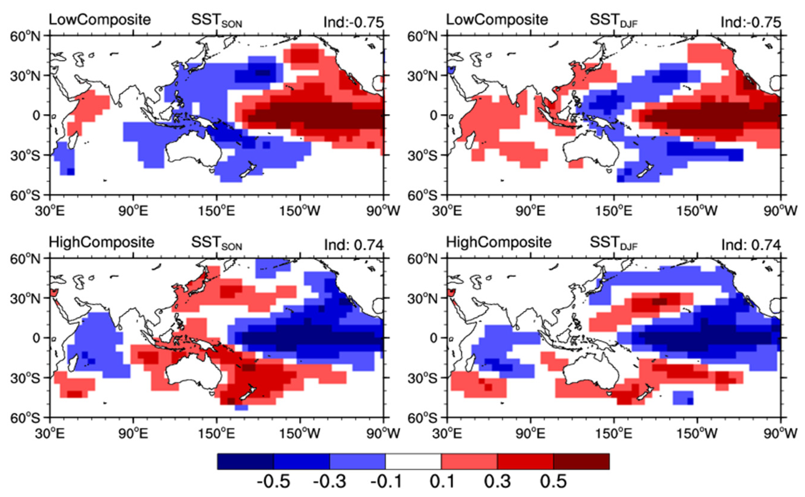
The SST shows an obvious decadal-scale warming trend due to global warming (not shown). This decadal-scale trend is removed by the 21-point (i.e., year) moving average method. The WPSHRL indexes are normalized to the range of −1 to 1. It is noteworthy that only the Pacific and Indian Ocean (60° S to 60° N, 30° E to 90° W) season-average (only autumn and winter) SST are used as input predictors. In order to increase the number of training data samples, we artificially produced some samples based on the composite analysis. Figure 1 presents the composites in the low (the lowest ~1/4) and high (the highest ~1/4) WPSHRL index years. This is consistent with previous studies in that the low composite and high composite are almost opposite, and the WPSHRL index is apt to be low/high if the pattern of prophase SST anomalies is similar to the low/high composite [37,38,39,40,41]. Furthermore, the WPSHRL index is assumed to be enhanced/weakened if the composited prophase SST anomalies are enhanced/weakened [35,42,43]. These conclusions were used as climatological background knowledge in this study. Based on this background knowledge, 20 extended samples were produced by magnifying or reducing the low composite data (SST field and corresponding WPSHRL index, upper panel of Figure 1). For example, both the SST field and corresponding WPSHRL index (i.e., −0.75) multiplied by 1.1 (or other values around 1.0) can produce an extended sample. Similarly, another 20 extended samples were produced by magnifying or reducing the high composite data (lower panel of Figure 1). Therefore, a total of 40 extended samples were used in the forecasting system.
2.2. Forecast System
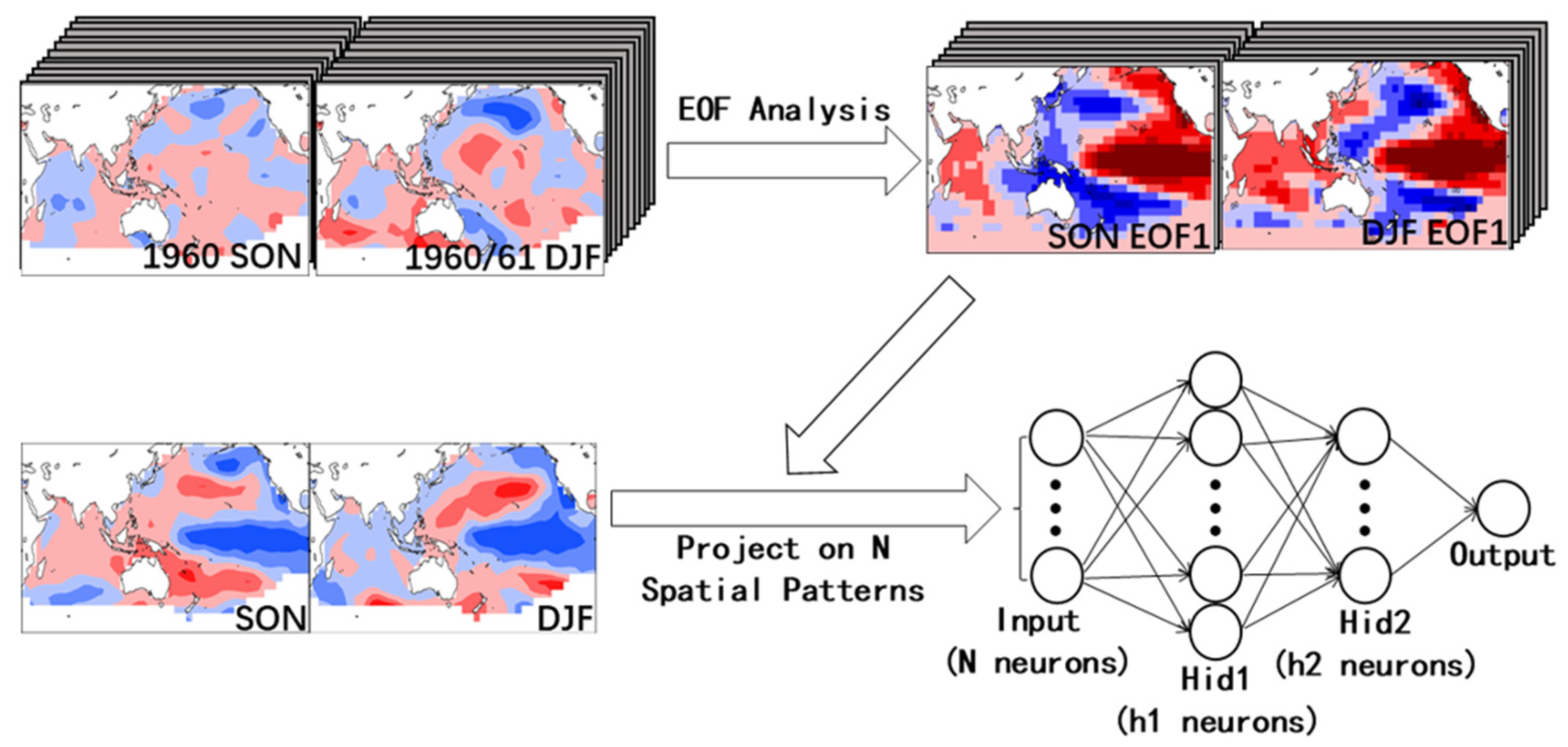
Figure 2 shows the architecture of the NN-based forecast system for the June WPSHRL indexes. The 20 leading empirical orthogonal function (EOF) eigenvectors of observed autumn and winter SST data from 1960 to 2021 are first stored as background knowledge. The N (N ≤ 20, tunable parameter) leading EOF principal components of the latest SST data are used as predictors (i.e., the input layer of the NN model). There are two hidden layers with tunable neuron numbers (h1 and h2). The model architecture is constrained by N, h1, and h2, which are called the model’s hyperparameters [25]. How to obtain the optimal architecture hyperparameters (i.e., N, h1, and h2) is discussed in the next section.
The NN model used here is the standard feed-forward multi-layer perceptron NN model. In order to minimize the root-mean-square-error (RMSE) between the predictions (i.e., outputs) and the targets (i.e., the observed WPSHRL indexes), the model’s parameters (i.e., the weights and biases associated with each layer) are adjusted through gradient descent [44]. During every update of the model’s parameters (i.e., the training phase), one-third of the training set (i.e., the batch size) is used to calculate the gradients. After every update with the training set (only the observed samples), the artificially-produced samples are also used for training the model. The initial biases are random values in the range from −0.01 to 0.01. The initial weights (i.e., the undetermined parameters of the NN model) are normally distributed, and their variance is regularized by the square root of the layer neuron number [45]. The initial learning rate is set to 0.001, and it can be adaptively adjusted during model training. As the training goes on, the model can be adjusted to best fit the given training set, which causes an overfitting problem. Usually, some samples are reserved as the test set to evaluate the overfitting problem. The training is stopped once the error (i.e., RMSE) from the test set begins to increase. Unfortunately, this common approach is not suited for this study because the total sample size is too small. Here, there is no test set. The NN model would stop training once the training error (i.e., the RMSE from the training set) is less than a threshold value (hereafter referred to as the stopping threshold, ST). How to set this hyperparameter (i.e., ST) is discussed in the next section.
The NN model is trained by the training set (i.e., all or part of the already existing samples). However, the NN model is actually estimated by the performance on new unseen examples (i.e., generalization problem). Usually, some samples are reserved as the validation set to evaluate the model’s forecast skill. Considering the small sample size in this study, the leave-one-out cross validation approach was used to quantify the forecast skill of the NN model [25,46]. Just as its name implies, one subset is chosen as the validation set and the rest of the subsets are used as the training set, and so on until all subsets have acted as the validation set. More details about the leave-one-out approach can be found in these studies [25,47]. In the forecast system developed in this study, the whole observed dataset (e.g., 1961~2021) is divided into 61 subsets, each containing one sample. Firstly, the model is trained based on the second to the sixty-first samples and the first prediction (i.e., the predicted 1961 WPSHRL index) is calculated with this model using the SST data from the first sample. Subsequently, the model is trained again based on the first and third to the sixty-first samples and the second prediction (i.e., the predicted 1962 WPSHRL index) is calculated with this new model using the SST data from the second sample. This procedure is repeated until the sixty-first prediction (i.e., the predicted 2021 WPSHRL index) has been calculated. Finally, the forecast skill of the NN model is evaluated by the Pearson linear correlation coefficient (Cor) between the predictions from 1961 to 2021 and their corresponding observations. Furthermore, since more attention should be paid to the obvious lower or higher years (i.e., abnormal years), the number of abnormal years, which are successfully predicted (Nyears), is also used to evaluate the model forecast skill. It is noteworthy that the Cor and Nyears actually represent the forecast skill of the model framework (i.e., the model’s hyperparameters are fixed, but the model’s parameters are undetermined) because the predictions from 1961 to 2021 are calculated by different NN models (i.e., the weights and biases of the model are different although the model framework is fixed).
The performance of a machine learning model might be sensitive to the random seed for weight initialization [48]. Our preliminary analysis shows that some good random seeds can often lead to a relatively higher forecast skill, and the model training often fails to reach the stopping threshold when starting with some bad random seeds. Aside from this random seed, there is another random seed that is used for the order of training data. In contrast to the weight initialization random seed, the impact of the training order random seed is negligible. In other words, the forecast skill of a given model framework (i.e., all hyperparameters have been fixed) is mainly influenced by the weight initialization random seed. Therefore, selecting good seeds is an important step in the model training process. In this step, a large number (e.g., 200 in this study) of weight initialization random seeds were carried out, and each seed corresponds to a model training forecast skill estimated by the leave-one-out approach. The reason for the name, “training forecast skill” is because the forecast skill is estimated based on the training set (i.e., during the training phase). In order to use the leave-one-out approach, one sample from the training set is chosen as the validation set and the other samples are used to train the model, and so on, until all samples from the training set have acted as the validation set. The best 10 random seeds are selected based on the training forecast skill (only the Cor). After that, the NN model would be trained again using these 10 good seeds (one seed corresponds to one NN model). In this step, the leave-one-out approach is not needed; thus, all samples from the training set are used to train the model. Finally, there are 10 NN models (the model’s parameters are fixed) in the forecast system, the actual prediction is the average of the 10 corresponding predictions (i.e., the ensemble-mean prediction). The standard deviation calculated from the difference in each prediction for 10 predictions is used to indicate the uncertainty of the ensemble-mean prediction to some extent. The main goal of ensemble prediction is to enhance the robustness of the forecast skills. In the rest of this article, the forecast skill usually denotes that which is calculated based on the ensemble-mean prediction. It is important to note that more details about the forecast system can be found in the code, which has been archived in a public repository.
3. Application and Evaluation
3.1. Setting Hyperparameters
All the hyperparameters must be set at the start of model training. Most of the time, setting hyperparameters requires an expensive guess-and-check process [25]. Similar to selecting good seeds, setting hyperparameters is also based on the model training forecast skill estimated by the leave-one-out approach. In this step, all observed samples are reserved as a training set, and the training forecast skill used for setting the hyperparameters is calculated based on the ensemble-mean prediction from the best 10 random seeds.
In this study, there is one hyperparameter for the model training (i.e., ST) and three hyperparameters for the model architecture (i.e., N, h1, and h2). The number of possible combinations is huge. Fortunately, the model performance is more sensitive to the hyperparameter of the input layer (i.e., N) as compared to other hyperparameters. Therefore, N should be set first. Table 1 lists the training forecast skills (Cor, Nyears) under different model architectures. It is obvious that the optimal N is 13 at ST = 0.36. We note that 13 is also the optimal value of N at other STs (e.g., 0.33 and 0.40, not shown). It seems that a small N (N < 13) cannot provide enough useful information, and a large N (N > 13) may cause a more serious overfitting problem.
After setting N, it becomes relatively simple to set the other hyperparameters. Table 2 lists the forecast skills under different combinations of the other three hyperparameters (i.e., ST, h1, and h2). Compared to the N, the impacts of the other hyperparameters on the forecast skill are not remarkable. Generally speaking, the model training phase is insufficient if the ST is too large, and the overfitting problem becomes serious if the ST is too small. Taken overall, the forecast skills at ST = 0.36 are a little better than those at other STs. Considering the generalization problem, a simple model is better than a complex model under similar forecast skills [25]. Based on the above analysis, the Cor = 0.67 and Nyears = 18 at ST = 0.36, h1 = 4 and h2 = 3 was taken as the best forecast skill, although the model framework (ST = 0.36, h1 = 4 and h2 = 4) produces the highest Nyears (Nyears = 19). In this study, N = 13, h1 = 4, h2 = 3 and ST = 0.36 were chosen as the optimal hyperparameters when the size of the training set is around 61. If the size of training set is far from 61, the optimal hyperparameters should be reset.
The training forecast skills analyzed above do not indicate the actual forecast skill of the forecast system. The training forecast skills are only used for setting hyperparameters and selecting random seeds. After that, the NN model is trained again using the whole training set. To some extent, the training forecast skill might be considered as the maximum potential forecast skill of the forecast system.
3.2. Forecast Skill
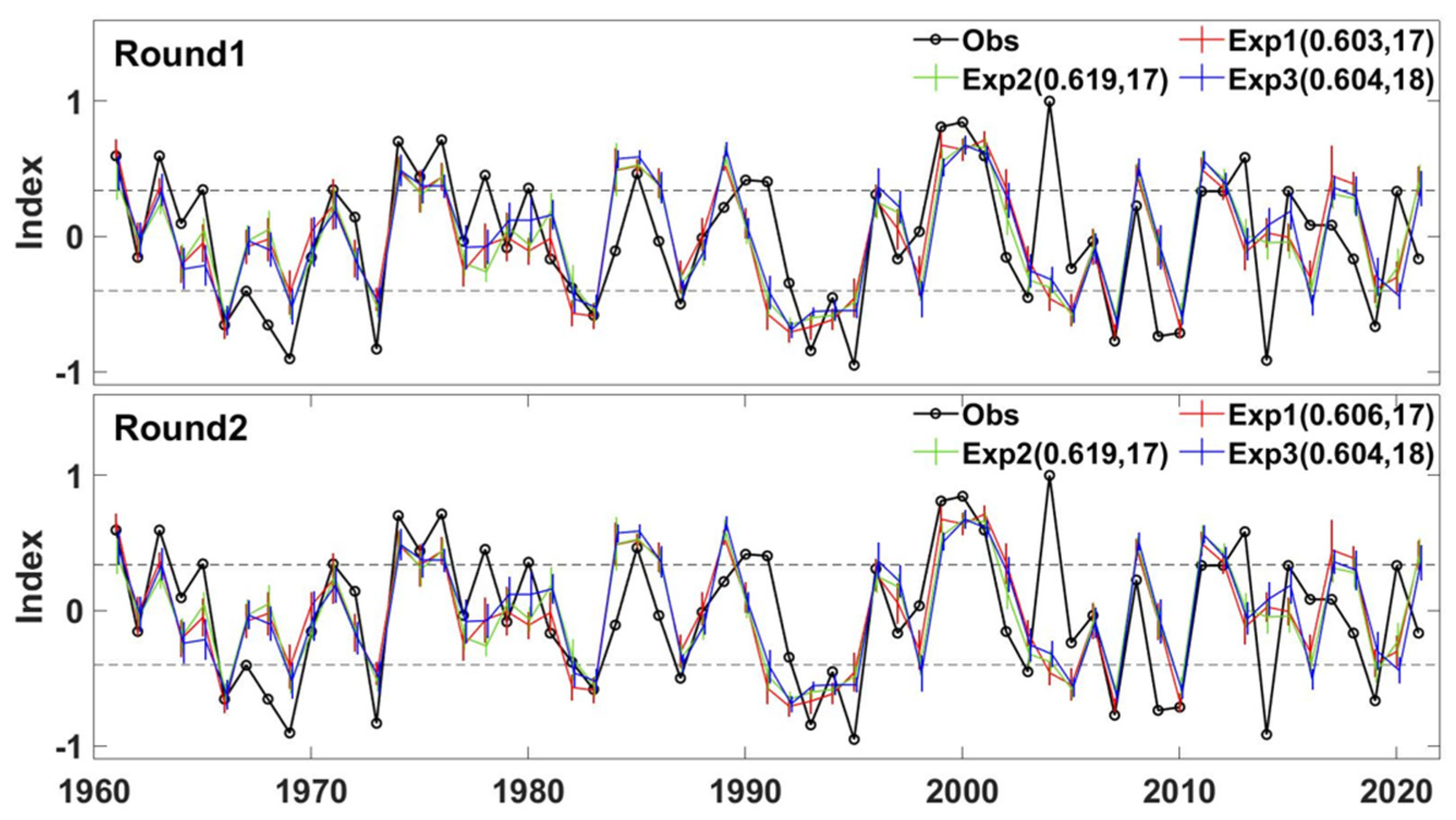
Firstly, the forecast skill of the forecast system was analyzed based on all observed samples (i.e., 1961~2021). The leave-one-out approach was used twice; once to calculate the training forecast skills during the model training phase (the number of available samples is 60), and again to calculate the actual forecast skill used for estimating the forecast system (the number of available samples is 61). Three forecast experiments, named Exp1, Exp2, and Exp3, were carried out with different selection ranges of weight initialization random seeds (e.g., 0~199, 400~599, and 1000~1199). The three forecast experiments (Exp1, Exp2, and Exp3) were run twice using the same code, named Round1 and Round2. The experimental results showed that the forecast system has acceptable predictability in most years (Figure 3). However, the predictability is always bad in a few years. For example, in 2004, the observed WPSHRL index is very high, although the spatial pattern of the prophase SST anomalies (not shown) is more similar to the composites of SST anomalies in low index years (Figure 1). In other words, 2004 is contrary to the background knowledge from the composite analysis (i.e., Figure 1). These years are called special years in this paper. It is very difficult to improve the predictability in these special years. Taken overall, the forecast skill of the forecast system is acceptable. The Cor is higher than 0.6 in all experiments. The number of abnormal years from observation is 30. The Nyears value is 17 or 18, which is around three-fifths of the observed abnormal years. This suggests that the forecast system is applicable to both normal years and abnormal years. Furthermore, the robustness of the forecast system was also analyzed. The prediction uncertainty, which is the standard deviation from the 10 ensemble members, is usually less than 0.2. As compared to the ensemble-mean value (i.e., the final prediction, which is in the range of −1 to 1), the uncertainty range (<0.2) is usually not significant. The difference in Cor and Nyears among the Exp1, Exp2, and Exp3 experiments is less than 0.02 and 2, respectively. The impact of the range of random seed selection is relatively small and negligible. The forecast skills from these three experiments are almost the same in Round1 ((0.603, 17), (0.619, 17), and (0.604, 18), respectively) and Round2 ((0.606, 17), (0.619, 17), and (0.604, 18), respectively). In terms of forecast skill, the forecast system is relatively stable, although the NN model’s parameters are different in these forecast experiments.
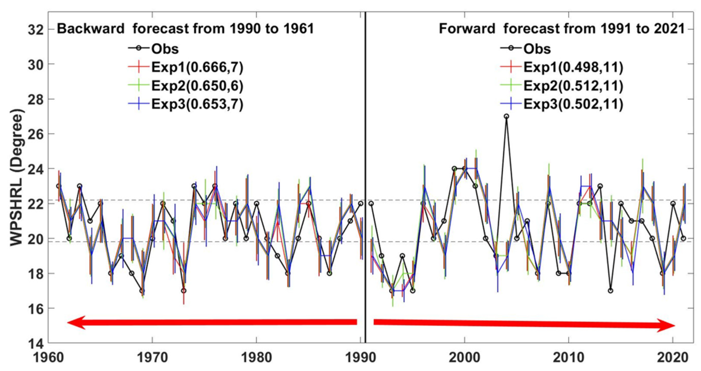
The forecast skill was also analyzed by applying the forecast system (Figure 4). In the forward forecast experiments, all available samples were used as a training set. Assuming it was 1 March 1998, the June 1998 WPSHRL was forecast using the NN models trained by the observed samples from 1961 to 1997. The backward forecast experiments were carried out under the assumption that the order of years is reversed. In these forecast experiments, the optimal hyperparameters of the NN model need to be reset based on the size of the corresponding training set, and the predicted WPSHRL indexes return back to the integer degree of latitude. The Cor is around 0.66 in the backward experiments from 1990 to 1961. In the forward experiments from 1991 to 2021, the Cor is obviously decreased due to a few special years (e.g., 2004, 2014). The Cor from the forward experiments without 2004 and 2014 is around 0.63 (not shown in Figure 4), which is close to that from the backward experiments. The reason that the forecast skill (evaluated by the Cor) for the June WPSHRL is decreased after 2000 might be that the special years occur more frequently. The numbers of observed abnormal years from the backward experiment period and forward experiment period are 12 and 15, respectively. Note that, the year with a WPSHRL higher than 22° N is taken as an abnormal year. In the backward experiment period, there are too many years (7) with the WPSHRL at the threshold value (22° N). This is the reason why the number of abnormal years from the backward experiment period is 3 less (i.e., 15–12) than that from the forward experiment period. The number of Nyears is 10 (two-thirds of the observed abnormal years) in the forward experiment period. Taken overall (i.e., 1961~2021), Nyear is 17 or 18, which is around three-fifths of the observed abnormal years. The forecast skill (both Cor and Nyears) estimated by this approach (Figure 4) is similar to that estimated by the leave-one-out approach (Figure 3).
3.3. Interpretability of the Forecast System
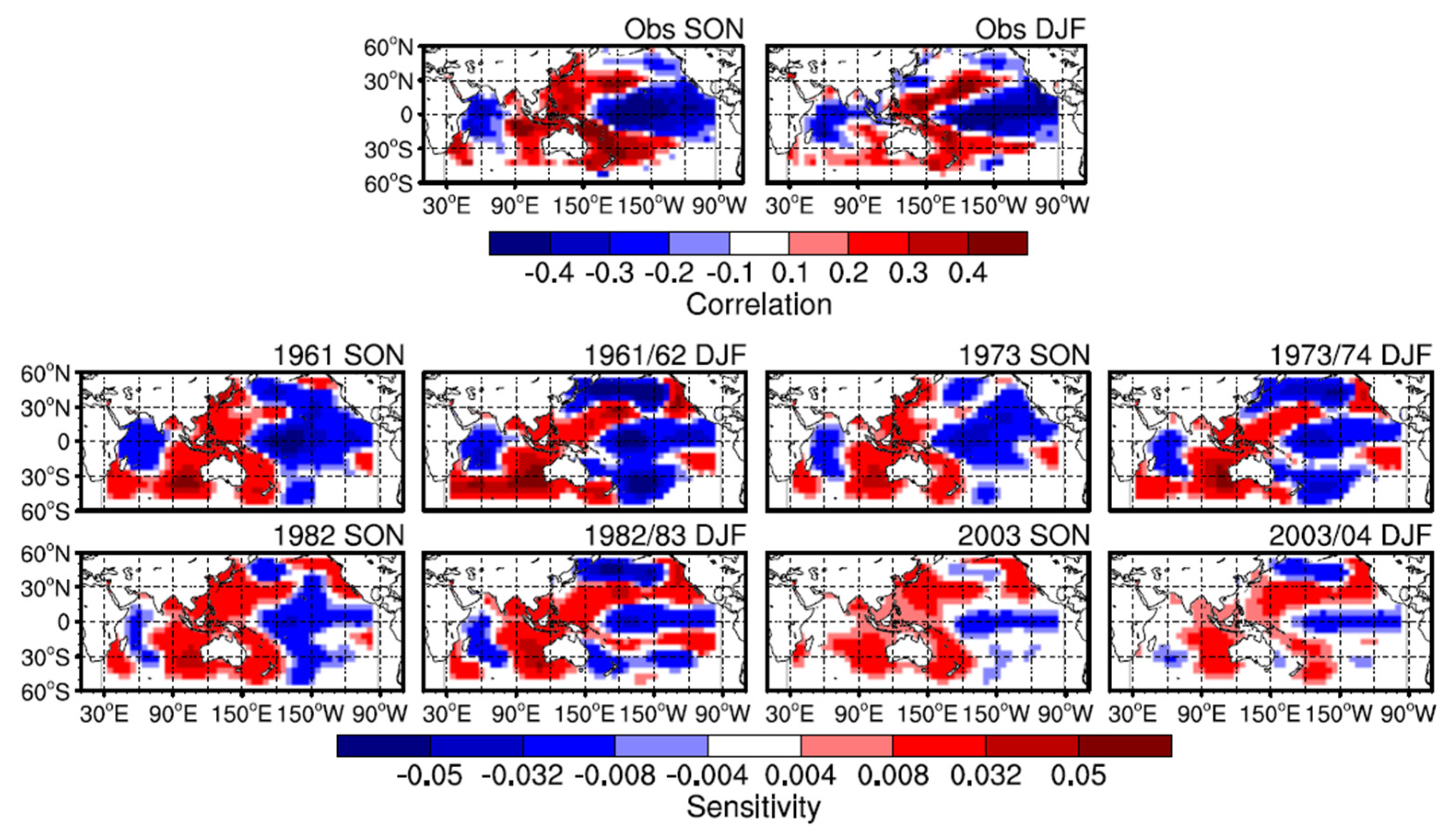
It is difficult to illustrate the physical interpretability of an NN model with several hidden layers. However, the perturbation-based method can be used to check the relation between input predictors and target predictands from the NN model [33,49]. Here, the interpretability of the forecast system was analyzed by the perturbation-based method. Figure 5 shows the sensitivity of the predicted WPSHRL to the prophase SST (i.e., ∂WPSHRL/∂SST). Here, the sensitivities were calculated based on the NN models (with given weights and biases) used in Figure 3 (Exp1 from Round1). The relationship between the SST and WPSHRL from the observation can be shown by the linear correlation (Figure 5, upper panel). Unlike the linear correlation from the observation, the sensitivity from the non-linear statistical model (i.e., the NN model) in one region (e.g., the North Pacific) is influenced by the SST in another region (e.g., the East Pacific). Therefore, the sensitivity from the NN model is dependent on the SST field of the year. The sensitivities of four years (1962, 1974, 1983 and 2004) are shown in Figure 5. The observed WPSHRL indexes from 1962, 1974, 1983, and 2004 are −0.15 (normal), 0.70 (high), −0.58 (low), and 1.00 (high), respectively. Their corresponding predicted WPSHRL indexes are −0.04 (normal), 0.51 (high), −0.56 (low), and −0.38 (normal), respectively. The years 1962, 1974, and 1983 have good predictions, whereas 2004 has a bad prediction. The spatial pattern of these sensitivities from the NN model is generally in agreement with the linear correlation from observation, especially for the years with good predictions. This is consistent with previous studies in that the SST anomalies of prophase autumn and winter might continue into summer [38,50], and increasing summer SST in the western Pacific warm pool would lead to a higher (more northerly) WPSHRL index [51,52,53]. The differences in sensitivity among these good years are not pronounced although the input SST fields (not shown) and predicted WPSHRL indexes (normal, high, and low) are obviously different. As compared to the sensitivities from these good years, the sensitivities from the bad year (i.e., 2004, the year with bad prediction) are relatively weak in most regions and the spatial pattern is very different from the linear correlation. These characteristics can also be found in most bad years (not shown). It seems necessary to check the sensitivity from the NN model, which is calculated based on the input SST data. The weak sensitivity and a bad spatial pattern usually indicate that the corresponding prediction is of low reliability.
4. Discussion
It is useful to discuss the experiences of climate prediction using machine learning methods from this study and previous researches. Unlike other application areas, there are two unique aspects in regard to climate prediction. One is that the size of the observed samples is very small (adverse condition), the other is that previous studies have provided a great deal of useful background knowledge (favorable condition).
Previous studies have provided some techniques to deal with the adverse condition [19,21,22,23,53]. For instance, Ham et al. (2019) used transfer learning to train a convolutional neural network (CNN), first on historical climate model simulations, and subsequently on reanalysis of SST data [19]. In addition, Wu et al. (2006) use a simple NN model to forecast the Pacific sea surface temperatures [23]. The NN model with dozens of parameters has fewer demands in regard to sample size as compared to the CNN model with thousands of parameters [25]. Furthermore, the transfer learning mothed could not be used in this study because climate models generally cannot forecast WPSHRL at a lead time of three months [14]. Therefore, the simple NN model was chosen in this study. It is also necessary to point out that one novelty of this study is the 40 extended samples, which were produced based on the composite analysis, following the idea from sample-extending technology used in other areas [54]. The 40 extended samples were very useful, and this improved the forecast skill by about 5%. This suggests that sample-extending technology has great potential in climate prediction.
Previous studies have also provided information on how to use the favorable condition (i.e., climatological background knowledge). For instance, the interpretability of the forecast model is checked by climatological background knowledge [19,53]. In this study, the interpretability of the NN model was also checked by climatological background knowledge (Figure 5). Unlike these previous studies, the recently reported perturbation-based method [33,49] was used in this study. This method has the advantages of simple coding and easy understanding because the interpretability only focuses on the relation between input predictors and target predictands. Furthermore, the climatological background knowledge was also used in other ways, such as the composite analysis (Figure 1), the selection of the regions of SST data as predictors (Figure 2), and the principal component extraction (Figure 2). Using a simple machine learning model, the forecast skill with the Pacific and Indian Ocean SST is obviously better than that with the global SST.
5. Conclusions
In this study, we developed a forecast system for the June WPSHRL index based on the latest autumn and winter SST. Considering the limited number of observed samples, a simple NN model was used to extract the non-linear relationship between input predictors and target predictands in the forecast system. The linear correlation coefficient between the predictions from the forecast system and their corresponding observations was around 0.6, and about three-fifths of the observed abnormal years were successfully predicted. Furthermore, sensitivity experiments (i.e., Exp1–3, Round1–2) show that the forecast system is relatively stable in terms of forecast skill. Therefore, we think that the forecast system would be valuable in real-life applications. The success of this forecast system suggests that the prediction of the atmospheric circulation indexes beyond one season might be improved by non-linear statistical methods (e.g., the NN model).
The practicability of the July and August WPSHRL index was also tested using this forecast system. The input predictors were still the latest autumn and winter SST. Although the forecast skill for the July WPSHRL was significantly reduced as compared to that for the June WPSHRL, the forecast skill was still acceptable (the Cor was around 0.40). However, the forecast skill for the August WPSHRL was very low (the Cor did not reach 0.3). It is well known that the formation mechanism for the WPSHRL index is different in different months [55,56]. The forecast system introduced in this study is designed only for the prediction of the June WPSHRL with a lead time of three months. For instance, the predictors (i.e., the regional and seasonal SST data) are first selected according to background knowledge (i.e., the strong linear correlation between the prophase SST and the June WPSHRL index). Generally speaking, the background knowledge from previous studies is useful for improving the performance of the forecast system. In order to make rational use of the background knowledge, the forecast system should be designed according to the month and lead time.
Author Contributions
X.S. designed the study. H.Y. supported the study. C.S. developed the forecast system and corresponding code. C.S. and X.S. wrote the original draft. Q.J. and Y.Z. contributed to reviewing and editing the manuscript. All authors have read and agreed to the published version of the manuscript.
Funding
This research was funded by the National Key Research and Development Program of China (grant nos. 2020YFA0608000) and the National Natural Science Foundation of China (grant nos. 41775095 and 42075145). The APC was funded by the same funders.
Institutional Review Board Statement
Not applicable.
Informed Consent Statement
Not applicable.
Data Availability Statement
The WPSHRL data from 1961 to 2016 are downloadable from http://cmdp.ncc-cma.net/160/74.php (accessed on 26 February 2022). The original SST data are downloadable from https://psl.noaa.gov/data/gridded/data.kaplan_sst.html (accessed on 26 February 2022). The code of the forecast system and related results used in this study have been archived in a public repository https://0-doi-org.brum.beds.ac.uk/10.5281/zenodo.6294926 (accessed on 26 February 2022).
Acknowledgments
The authors would like to thank Dong Si for guidance in the calculation method for the WPSHRL index. This study was conducted in the High-Performance Computing Center of Nanjing University of Information Science & Technology.
Conflicts of Interest
The authors declare no conflict of interest.
References
- Tao, S.; Wei, J. The Westward, Northward advance of the Subtropical High over the West Pacific in Summer. J. Appl. Meteor. Sci. 2006, 17, 513–525. [Google Scholar] [CrossRef]
- Liu, Y.; Hong, J.; Liu, C.; Zhang, P. Meiyu flooding of Huaihe River valley and anomaly of seasonal variation of subtropical anticyclone over the Western Pacific. Chin. J. Atmos. Sci. 2013, 37, 439–450. [Google Scholar]
- Yu, Y.; Wang, S.; Qian, Z.; Song, M.; Wang, A. Climatic linkages between SHWP position and EASM Rainy-Belts and-Areas in east part of China in summer half year. Plateau Meteor. 2013, 32, 1510–1525. Available online: http://www.gyqx.ac.cn/CN/10.7522/j.issn.1000-0534.2013.00033 (accessed on 26 February 2022).
- Wu, S.; Guo, D. Effects of East Asian summer monsoon and Western Pacific Subtropical High on summer precipitation in China. Sci. Technol. Innov. Herald. 2019, 16, 112–119. [Google Scholar] [CrossRef]
- Zhang, E.; Tang, B.; Han, Z. A long-range forecasting model for the Subtropical High using the integral multi-level recursion. J. Appl. Meteor. Sci. 1989, 4, 69–74. Available online: http://qikan.camscma.cn/article/id/19890110 (accessed on 26 February 2022).
- Dong, Z.; Zhang, R. A prediction of the Western Pacific Subtropical High based on wavelet decomposition and ANFIS model. J. Trop. Meteor. 2004, 20, 419–425. [Google Scholar] [CrossRef]
- Ren, H.; Zhang, P.; Guo, B.; Chou, J. Dynamical model of Subtropical High ridge-line section and numerical simulations with its simplified scheme. Chin. J. Atmos. Sci. 2005, 29, 71–78. [Google Scholar]
- Zhang, R.; Wang, H.; Liu, K.; Hong, M.; Yu, D. Dynamic randomicity and complexity of Subtropical High index based on phase space reconstruction. J. Nanjing Inst. Meteor. 2007, 30, 723–729. [Google Scholar] [CrossRef]
- Wang, Y.; Teng, J.; Zhang, R.; Wan, Q.; Dong, Z.; Bai, Z. Predicting the Subtropical High index by coupling self-organizing feature map and generalized regression neural network. J. Trop. Meteor. 2008, 24, 475–482. [Google Scholar] [CrossRef]
- Fu, B.; Wang, T.; Wei, C.; Deng, Z. Testing and assessment of capabilities of day-to-day predicting of summertime West Pacific Subtropical High based on CFSv2. Guangdong Meteor. 2016, 38, 15–19. [Google Scholar] [CrossRef]
- Duan, C.; Xu, M.; Cheng, Z.; Luo, L. Evaluation on monthly prediction of Western Pacific Subtropical High by DERF2.0 model. Meteor. Mon. 2017, 43, 1267–1277. Available online: https://d.wanfangdata.com.cn/periodical/qx201710011 (accessed on 26 February 2022).
- Qian, D.; Guan, Z.; Xu, J. Prediction models for summertime Western Pacific Subtropical High based on the leading SSTA modes in the tropical Indo-Pacific sector. Trans. Atmos. Sci. 2021, 44, 405–417. [Google Scholar] [CrossRef]
- Jia, Y.; Hu, Y.; Zhong, Z.; Zhu, Y. Statistical forecast model of Western Pacific Subtropical High indices in Summer. Plateau Meteor. 2015, 34, 1369–1378. Available online: http://www.gyqx.ac.cn/CN/10.7522/j.issn.1000-0534.2014.00079 (accessed on 26 February 2022).
- Zhou, F.; Ren, H.; Hu, Z.; Liu, M.; Wu, J.; Liu, C. Seasonal predictability of primary East Asian Summer circulation patterns by three operational climate prediction models. Quart. J. Roy. Meteor. Soc. 2020, 146, 629–646. [Google Scholar] [CrossRef]
- Kalnay, E. Atmospheric Modeling, Data Assimilation and Predictability, 1st ed.; Cambridge University Press: Cambridge, UK, 2002; pp. 1–27. [Google Scholar] [CrossRef]
- Huntingford, C.; Jeffers, E.S.; Bonsall, M.B.; Christensen, H.M.; Lees, T.; Yang, H. Machine learning and artificial intelligence to aid climate change research and preparedness. Environ. Res. Lett. 2019, 14, 124007. [Google Scholar] [CrossRef] [Green Version]
- Reichstein, M.; Camps-Valls, G.; Stevens, B.; Jung, M.; Denzler, J.; Carvalhais, N.; Prabhat. Deep learning and process understanding for data-driven Earth system science. Nature 2019, 566, 195–204. [Google Scholar] [CrossRef]
- He, S.; Wang, H.; Li, H.; Zhao, J. Machine learning and its potential application to climate prediction. Trans. Atmos. Sci. 2021, 44, 26–38. Available online: http://dx.chinadoi.cn/10.13878/j.cnki.dqkxxb.20201125001 (accessed on 26 February 2022).
- Ham, Y.G.; Kim, J.H.; Luo, J.J. Deep learning for multi-year ENSO forecasts. Nature 2019, 573, 568–572. [Google Scholar] [CrossRef]
- Geng, H.; Wang, T. Spatiotemporal model based on deep learning for ENSO forecasts. Atmosphere 2021, 12, 810. [Google Scholar] [CrossRef]
- Tangang, F.T.; Hsieh, W.W.; Tang, B. Forecasting the equatorial Pacific sea surface temperatures by neural network models. Climate Dyn. 1997, 13, 135–147. [Google Scholar] [CrossRef]
- Tangang, F.T.; Hsieh, W.W.; Tang, B. Forecasting regional sea surface temperatures in the tropical Pacific by neural network models, with wind stress and sea level pressure as predictors. J. Geophys. Res. 1998, 103, 7511–7522. [Google Scholar] [CrossRef]
- Wu, A.; Hsieh, W.W.; Tang, B. Neural network forecasts of the tropical Pacific sea surface temperatures. Neural Netw. 2006, 19, 145–154. [Google Scholar] [CrossRef] [PubMed] [Green Version]
- Abdullah, S.; Ismail, M.; Ahmed, A.N.; Abdullah, A.M. Forecasting particulate matter concentration using linear and non-Linear approaches for air quality decision support. Atmosphere 2019, 10, 667. [Google Scholar] [CrossRef] [Green Version]
- Goodfellow, I.; Bengio, Y.; Courville, A. Deep Learning; MIT Press: Cambridge, CA, USA, 2016; pp. 89–223. Available online: http://www.deeplearningbook.org (accessed on 26 February 2022).
- Tran, T.; Lee, T.; Kim, J.S. Increasing Neurons or Deepening Layers in Forecasting Maximum Temperature Time Series? Atmosphere 2020, 11, 1072. [Google Scholar] [CrossRef]
- Ribeiro, M.T.; Singh, S.; Guestrin, C. “Why Should I Trust You?”: Explaining the Predictions of Any Classifier. arXiv 2016, arXiv:1602.04938. [Google Scholar] [CrossRef]
- Fong, R.; Vedaldi, A. Interpretable explanations of black boxes by meaningful perturbation. arXiv 2017, arXiv:1704.03296. [Google Scholar] [CrossRef]
- Kindermans, P.J.; Schütt, K.T.; Alber, M.; Müller, K.R.; Erhan, D.; Kim, B.; Dähne, S. Learning how to explain neural networks: PatternNet and PatternAttribution. arXiv 2017, arXiv:1705.05598. [Google Scholar] [CrossRef]
- Guidotti, R.; Monreale, A.; Ruggieri, S.; Turini, F.; Giannotti, F.; Pedreschi, D. A survey of methods for explaining black box models. ACM Comput. Surv. 2019, 51, 1–42. [Google Scholar] [CrossRef] [Green Version]
- Fan, F.; Xiong, J.; Li, M.; Wang, G. On Interpretability of Artificial Neural Networks: A Survey. arXiv 2020, arXiv:2001.02522. [Google Scholar] [CrossRef]
- Belochitski, A.; Krasnopolsky, V. Robustness of neural network emulations of radiative transfer parameterizations in a state-of-the-art general circulation model. Geosci. Model Dev. 2021, 14, 7425–7437. [Google Scholar] [CrossRef]
- Yuan, H.; Yu, H.; Gui, S.; Ji, S. Explainability in Graph Neural Networks: A Taxonomic Survey. arXiv 2021, arXiv:2012.15445. [Google Scholar] [CrossRef]
- Kaplan, A.; Cane, M.A.; Kushnir, Y.; Clement, A.C.; Blumenthal, M.B.; Rajagopalan, B. Analyses of global sea surface temperature 1856–1991. J. Geophys. Res. 1998, 103, 18567–18589. [Google Scholar] [CrossRef] [Green Version]
- Yao, Y.; Yan, H. Relationship between proceeding pacific sea surface temperature and Subtropical High indexes of main raining seasons. J. Trop. Meteor. 2008, 24, 483–489. [Google Scholar] [CrossRef]
- Liu, Y.; Li, W.; Ai, W.; Li, Q. Reconstruction and application of the monthly Western Pacific Subtropical High indices. J. Appl. Meteor. Sci. 2012, 23, 414–423. [Google Scholar]
- Chen, L. Interaction between the subtropical high over the north Pacific and the sea surface temperature of the eastern equatorial Pacific. Chin. J. Atmos. Sci. 1982, 6, 148–156. [Google Scholar]
- Ying, M.; Sun, S. A Study on the Response of Subtropical High over the Western Pacific the SST Anomaly. Chin. J. Atmos. Sci. 2000, 24, 193–206. [Google Scholar] [CrossRef]
- Zeng, G.; Sun, Z.; Lin, Z.; Ni, D. Numerical Simulation of Impacts of Sea Surface Temperature Anomaly upon the Interdecadal Variation in the Northwestern Pacific Subtropical High. Chin. J. Atmos. Sci. 2010, 34, 307–322. [Google Scholar] [CrossRef]
- Ong-Hua, S.; Feng, X. Two northward jumps of the summertime western pacific subtropical high and their associations with the tropical SST anomalies. Atmos. Ocean. Sci. Lett. 2011, 4, 98–102. [Google Scholar] [CrossRef] [Green Version]
- Xue, F.; Zhao, J. Intraseasonal variation of the East Asian summer monsoon in La Niña years. Atmos. Ocean. Sci. Lett. 2017, 10, 156–161. [Google Scholar] [CrossRef] [Green Version]
- Huang, R.; Sun, F. Impacts of the Thermal State and the Convective Activities in the Tropical Western Warm Pool on the Summer Climate Anomalies in East Asia. Chin. J. Atmos. Sci. 1994, 18, 141–151. [Google Scholar] [CrossRef]
- Ai, Y.; Chen, X. Analysis of the correlation between the Subtropical High over Western Pacific in Summer and SST. J. Trop. Meteor. 2000, 16, 1–8. [Google Scholar] [CrossRef]
- Hornik, K.; Stinchcombe, M.; White, H. Multilayer Feedforward Networks are Universal Approximators. Neur. Netw. 1989, 2, 359–366. [Google Scholar] [CrossRef]
- Glorot, X.; Bengio, Y. Understanding the difficulty of training deep feedforward neural networks. In Proceedings of the Thirteenth International Conference on Artificial Intelligence and Statistics, Sardinia, Italy, 13–15 May 2010; pp. 249–256. [Google Scholar]
- Opper, M.; Winther, O. Gaussian Processes and SVM: Mean Field Results and Leave-One-Out. Advances in Large Margin Classifiers, 8th ed.; Smola, A.J., Bartlett, P.L., Schölkopf, B., Schuurmans, D., Eds.; MIT Press: Cambridge, CA, USA, 2000; pp. 311–326. Available online: https://www.researchgate.net/publication/40498234 (accessed on 26 February 2022).
- Volpe, V.; Manzoni, S.; Marani, M. Leave-One-Out Cross-Validation. In Encyclopedia of Machine Learning; Sammut, C., Webb, G.I., Eds.; Springer: Boston, MA, USA, 2011; pp. 24–45. [Google Scholar] [CrossRef]
- Dodge, J.; Ilharco, G.; Schwartz, R.; Farhadi, A.; Hajishirzi, H.; Smith, N. Fine-tuning pretrained language models: Weight initializations, data orders, and early stopping. arXiv 2020, arXiv:2002.06305. [Google Scholar] [CrossRef]
- Toms, B.A.; Barnes, E.A.; Ebert-Uphoff, I. Physically interpretable neural networks for the geosciences: Applications to earth system variability. arXiv 2020, arXiv:1912.01752. [Google Scholar] [CrossRef]
- Chen, D.; Gao, S.; Chen, J.; Gao, S. The synergistic effect of SSTA between the equatorial eastern Pacific and the Indian-South China Sea warm pool region influence on the western Pacific subtropical high. Haiyang Xuebao 2016, 38, 1–15. Available online: http://dx.chinadoi.cn/10.3969/j.issn.0253-4193.2016.02.001 (accessed on 26 February 2022).
- Tsuyoshi, N. Convective Activities in the Tropical Western Pacific and Their Impact on the Northern Hemisphere Summer Circulation. J. Meteor. Soc. Jpn. Ser. II 1987, 65, 373–390. [Google Scholar] [CrossRef] [Green Version]
- Huang, R.; Li, W. Influence of heat source anomaly over the western tropical Pacific on the subtropical high over East Asia and its physical mechanism. Chin. J. Atmos. Sci. 1988, 12, 107–116. [Google Scholar] [CrossRef]
- Liu, J.; Tang, Y.; Wu, Y.; Li, T.; Wang, Q.; Chen, D. Forecasting the Indian Ocean Dipole with deep learning techniques. Geophys. Res. Lett. 2021, 48, e2021GL094407. [Google Scholar] [CrossRef]
- Shorten, C.; Khoshgoftaar, T.M. A survey on image data augmentation for deep learning. J. Big Data 2019, 6, 60. [Google Scholar] [CrossRef]
- Qian, Q.; Liang, P.; Qi, L. Advances in the Study of Intraseasonal Activity and Variation of Western Pacific Subtropical High. Meteor. Environ. Sci. 2021, 44, 93–101. [Google Scholar] [CrossRef]
- Wen, M.; He, J. Ridge Movement and Potential Mechanism of Western Pacific Subtropical High in Summer. Trans. Atmos. Sci. 2002, 25, 289–297. Available online: http://dx.chinadoi.cn/10.3969/j.issn.1674-7097.2002.03.001 (accessed on 26 February 2022).
Figure 1.
Composites of the prophase autumn (SON, left) and winter (DJF, right) sea surface temperature (SST) anomalies in low (upper panel) and high (lower panel) WPSHRL index years. The corresponding low and high composite WPSHRL indexes are −0.75 and 0.74, respectively (upper right corner).
Figure 1.
Composites of the prophase autumn (SON, left) and winter (DJF, right) sea surface temperature (SST) anomalies in low (upper panel) and high (lower panel) WPSHRL index years. The corresponding low and high composite WPSHRL indexes are −0.75 and 0.74, respectively (upper right corner).

Figure 2.
Architecture of the NN-based model used for the June WPSHRL index forecast. The 20 leading EOF eigenvectors of observed SON and DJF SST data from 1960 to 2021 are stored as background knowledge. The N (N ≤ 20, tunable parameter) leading principal components of input SST (a certain year) obtained by calculating the pattern projection coefficients onto the EOF eigenvectors are used as predictors. The number of hidden layers is two, and the number of neurons at each hidden layer (h1, h2) is also a tunable parameter. The activation function is a hyperbolic tangent function.

Figure 3.
Time series of the WPSHRL index from the observations (black line) and model predictions (colored lines, for different experiments) for the period from 1961 to 2021. The vertical bars indicate the ranges of prediction uncertainty at different years. The dashed lines indicate the index thresholds for abnormal years. The three forecast experiments (Exp1, Exp2, and Exp3) were run twice using the same code (upper panel from Round1, and lower panel from Round2). Forecast skills (Cor, Nyears) are shown after the corresponding experiment names.

Figure 4.
Similar to Figure 3, but for the forward and backward forecast experiments. The number of the observed abnormal years from the above two periods (1961~1990 and 1991~2021) are 12 and 15, respectively.
Figure 4.
Similar to Figure 3, but for the forward and backward forecast experiments. The number of the observed abnormal years from the above two periods (1961~1990 and 1991~2021) are 12 and 15, respectively.

Figure 5.
The impact of the prophase SST on the June WPSHRL index from the observation (linear correlation, upper panel) and forecast system (sensitivities, lower panel).
Figure 5.
The impact of the prophase SST on the June WPSHRL index from the observation (linear correlation, upper panel) and forecast system (sensitivities, lower panel).


Table 1.
Training forecast skills (Cor, Nyears) under different model architectures (N, h1, and h2).
Table 1.
Training forecast skills (Cor, Nyears) under different model architectures (N, h1, and h2).
| N\(h1, h2) | (8, 5) | (6, 5) | (6, 4) | (4, 4) | (6, 3) | (4, 3) | (3, 3) |
|---|---|---|---|---|---|---|---|
| 8 | 0.56, 14 | 0.55, 16 | 0.57, 16 | 0.57, 16 | 0.56, 17 | 0.57, 16 | 0.57, 17 |
| 10 | 0.61, 17 | 0.60, 19 | 0.62, 18 | 0.59, 18 | 0.62, 18 | 0.59, 17 | 0.61, 19 |
| 12 | 0.62, 16 | 0.56, 18 | 0.62, 17 | 0.59, 18 | 0.59, 17 | 0.61, 17 | 0.60, 16 |
| 13 | 0.65, 18 | 0.64, 18 | 0.66, 18 | 0.64, 19 | 0.65, 17 | 0.67, 18 | 0.66, 18 |
| 14 | 0.64, 14 | 0.62, 18 | 0.63, 18 | 0.61, 19 | 0.62, 17 | 0.63, 19 | 0.64, 17 |
| 16 | 0.64, 18 | 0.63, 17 | 0.62, 17 | 0.63, 17 | 0.61, 17 | 0.63, 15 | 0.61, 18 |
| 18 | 0.63, 15 | 0.61, 16 | 0.61, 13 | 0.62, 18 | 0.60, 16 | 0.61, 12 | 0.62, 18 |
Here, the ST is set to 0.36, and the observed samples from 1961 to 2021 are used as the training set. The number of abnormal years from observation is 30.
Table 2.
Similar to Table 1, but for the training forecast skills (Cor, Nyears) under different stopping thresholds (ST) and hidden layer architectures (h1 and h2).
Table 2.
Similar to Table 1, but for the training forecast skills (Cor, Nyears) under different stopping thresholds (ST) and hidden layer architectures (h1 and h2).
| ST\(h1, h2) | (8, 5) | (6, 5) | (6, 4) | (4, 4) | (6, 3) | (4, 3) | (3, 3) |
|---|---|---|---|---|---|---|---|
| 0.28 | 0.64, 15 | 0.63, 14 | 0.64, 14 | 0.62, 17 | 0.65, 17 | 0.64, 16 | 0.65, 16 |
| 0.30 | 0.65, 15 | 0.64, 15 | 0.65, 14 | 0.62, 18 | 0.65, 18 | 0.65, 16 | 0.65, 16 |
| 0.34 | 0.66, 18 | 0.64, 16 | 0.66, 17 | 0.64, 19 | 0.65, 18 | 0.65, 18 | 0.66, 18 |
| 0.36 | 0.65, 18 | 0.64, 18 | 0.66, 18 | 0.64, 19 | 0.65, 17 | 0.67, 18 | 0.66, 18 |
| 0.38 | 0.66, 16 | 0.64, 17 | 0.66, 16 | 0.65, 18 | 0.65, 16 | 0.66, 16 | 0.65, 18 |
| 0.40 | 0.66, 15 | 0.64, 17 | 0.66, 17 | 0.65, 16 | 0.66, 18 | 0.65, 16 | 0.64, 16 |
| 0.42 | 0.67, 16 | 0.63, 18 | 0.67, 16 | 0.63, 18 | 0.64, 16 | 0.67, 15 | 0.65, 17 |
| 0.44 | 0.65, 14 | 0.61, 16 | 0.66, 15 | 0.61, 16 | 0.63, 16 | 0.66, 15 | 0.64, 16 |
Here, the N is set to 13.
Publisher’s Note: MDPI stays neutral with regard to jurisdictional claims in published maps and institutional affiliations. |
© 2022 by the authors. Licensee MDPI, Basel, Switzerland. This article is an open access article distributed under the terms and conditions of the Creative Commons Attribution (CC BY) license (https://creativecommons.org/licenses/by/4.0/).
Share and Cite
MDPI and ACS Style
Sun, C.; Shi, X.; Yan, H.; Jiang, Q.; Zeng, Y. Forecasting the June Ridge Line of the Western Pacific Subtropical High with a Machine Learning Method. Atmosphere 2022, 13, 660. https://0-doi-org.brum.beds.ac.uk/10.3390/atmos13050660
AMA Style
Sun C, Shi X, Yan H, Jiang Q, Zeng Y. Forecasting the June Ridge Line of the Western Pacific Subtropical High with a Machine Learning Method. Atmosphere. 2022; 13(5):660. https://0-doi-org.brum.beds.ac.uk/10.3390/atmos13050660
Chicago/Turabian StyleSun, Cunyong, Xiangjun Shi, Huiping Yan, Qixiao Jiang, and Yuxi Zeng. 2022. "Forecasting the June Ridge Line of the Western Pacific Subtropical High with a Machine Learning Method" Atmosphere 13, no. 5: 660. https://0-doi-org.brum.beds.ac.uk/10.3390/atmos13050660
Note that from the first issue of 2016, this journal uses article numbers instead of page numbers. See further details here.