Automated Recognition of Macro Downburst Using Doppler Weather Radar

Abstract

In light of the macro downburst’s ground divergent flow field characteristics and high reflectivity, this paper proposes an algorithm for identifying the downburst area using a Doppler weather radar low-level radial velocity and reflectivity factor (abbreviated as reflectivity, the same below). To binarize the radial velocity, perform quality control on the radial velocity and reflectivity, then combine the reflectivity and the radial velocity threshold. Following that, use the Eight-Neighborhood method to retrieve the positive and negative velocity connected regions and perform the connected regions. The positive and negative velocity pairs are then matched, and the zero Doppler velocity line between the positive and negative velocity pairs is extracted, followed by the center recognition of the positive and negative velocity downburst areas. The data of downbursts detected by Doppler radar in Jinan, Shandong Province, are used for algorithm verification in this paper. The results show that the proposed algorithm can detect the macro downburst area and identify the downburst center.

1. Introduction

In 1978, Fujita defined a downburst as a strong downdraft that causes strong catastrophic winds on or near the ground and subdivided the downburst into macro and micro downbursts based on the horizontal scale of the ground gale generated by the downburst [1,2]. The outflow level of a macro downburst is greater than 4 km. The macro downburst has the potential to produce strong ground winds of up to 60 m/s for 5 to 30 min, causing divergent damage on the ground. The outflow level of a micro downburst is less than 4 km. The micro downburst has the potential to produce strong ground winds of up to 75 m/s because of its small horizontal scale and high wind velocity. The micro downburst will cause significant wind shear at low levels, posing serious flight safety risks. Downbursts are classified as dry or macro based on whether or not precipitation falls on the ground during their occurrence. Macro downburst: when a microburst occurs, the precipitation exceeds 0.25 mm. The macro downburst is caused by the cold downdraft in the heavy precipitation. Dry downburst: the precipitation during the occurrence of a microburst is less than 0.25 mm. Dry downbursts are common in strong storms, owing to ice crystals in the cloud sinking into a relatively dry environment and quickly evaporating, resulting in a strong sinking cold air mass, which then sinks to the surface layer and diverges to the surroundings. Downbursts are classified according to echo patterns, which can be divided into a squall line, linear convection (except squall line), and nonlinear convective storm [3].

Downburst has always been a problem of short-term nowcasting and early warning due to its small scale, short life cycle, and high mobility. The temporal and spatial resolution of Doppler weather radar data is very high. As a result, the Doppler weather radar has become an effective means of monitoring and warning of downbursts. At present, both domestic and foreign researchers are working on identifying downbursts. Merritt [4] proposed a downburst detection algorithm based on shear segment extraction in 1987. To begin, look for the velocity shear section that satisfies the velocity difference greater than 20 m/s along the radial direction. After searching all the radial shear sections at the same elevation angle, combine the shear sections that are adjacent in azimuth and meet certain conditions in a dangerous area. If the dangerous area of the downburst stream reaches or exceeds a certain threshold, an alarm is triggered to hit the dangerous area. Roberts et al. [5] investigated whether the rapid fall of the reflectivity nucleus and the reflectivity notch could be used to warn of a downburst in 1989. In 1994, Wolfson et al. [6] proposed the automated microburst wind-shear prediction algorithm. The algorithm tracks the growth and dissipation characteristics of the monomer using a two-dimensional image processing method and can warn of downbursts with an outflow strength exceeding 15.4 m/s. In 2004, Smith et al. [7] proposed a catastrophic downburst forecast and detection algorithm. The algorithm establishes a forecast equation for downbursts using 26 parameters based on monomer reflectivity, radial velocity, and environmental parameters, and then issues early warnings for downbursts following the National Weather Service’s strong wind standards. From 1989 to 2014, Tuttle, Herzegh, Kumjian et al. [8,9,10] researched and proposed that the height and position of the ZDR column represent the strength and approximate position of the storm updraft, respectively. In 2021, Kuster et al. [11] studied the KDP cores in 81 different downburst data in 10 states and proposed that the KDP core can be used as a signal for predicting downbursts.

With the deployment of Doppler weather radar with Doppler velocity measurement function in China, Chinese scholars have launched observation and research on downbursts. Yu et al. [12] conducted the first detailed analysis of a series of downbursts using China’s new-generation weather radar data in 2006. Zhao et al. [13] summarized the status of Doppler weather radar identification and early warning of downbursts in 2007, providing a reference for domestic downburst research. In 2011, Tao et al. [14] proposed an automatic identification algorithm for downburst based on the core drop of the downburst reflectivity and the flow field characteristics of strong low-level radiation. In 2015, Du et al. [15] proposed an algorithm suitable for the identification of micro downbursts, and this algorithm has a strong identification effect on the downbursts with asymmetric divergence. Zhao [16] proposed a method for detecting and forecasting downbursts based on the static and dynamic properties of sequence fragments (time windows) in 2018. In 2019, based on the downburst warning indicators, including the characteristics of the environment, reflectivity, and radial velocity, Sun et al. [17] used Bayes and BP neural network methods to establish downburst forecast models. In 2019, Wang et al. [18] proposed a downburst warning method based on radar data extrapolation and feature recognition.

Based on the algorithm proposed by Du [15], this paper improves the algorithm for downburst region identification based on image processing using a single Doppler weather radar low-level radial velocity and reflectivity data for macro downburst. First, this paper lowers the threshold for radial velocity binarization, thereby increasing the detection probability of positive and negative velocity regions. Second, a new algorithm is added to identify the center of the downburst region, which will be introduced in Section 3.

2. Doppler Weather Radar Data Preprocessing

Doppler weather radar data is easily affected by ground objects, noise, and other factors, so effective quality control is required before radar data is used. To improve the quality of reflectivity, firstly remove isolated points and then make interpolation for the data of reflectivity. To improve the quality of radial velocity, firstly remove isolated points; secondly, filter the data of radial velocity; then reduces velocity ambiguity; finally, make interpolation for the data of radial velocity.

2.1. Remove Isolated Points

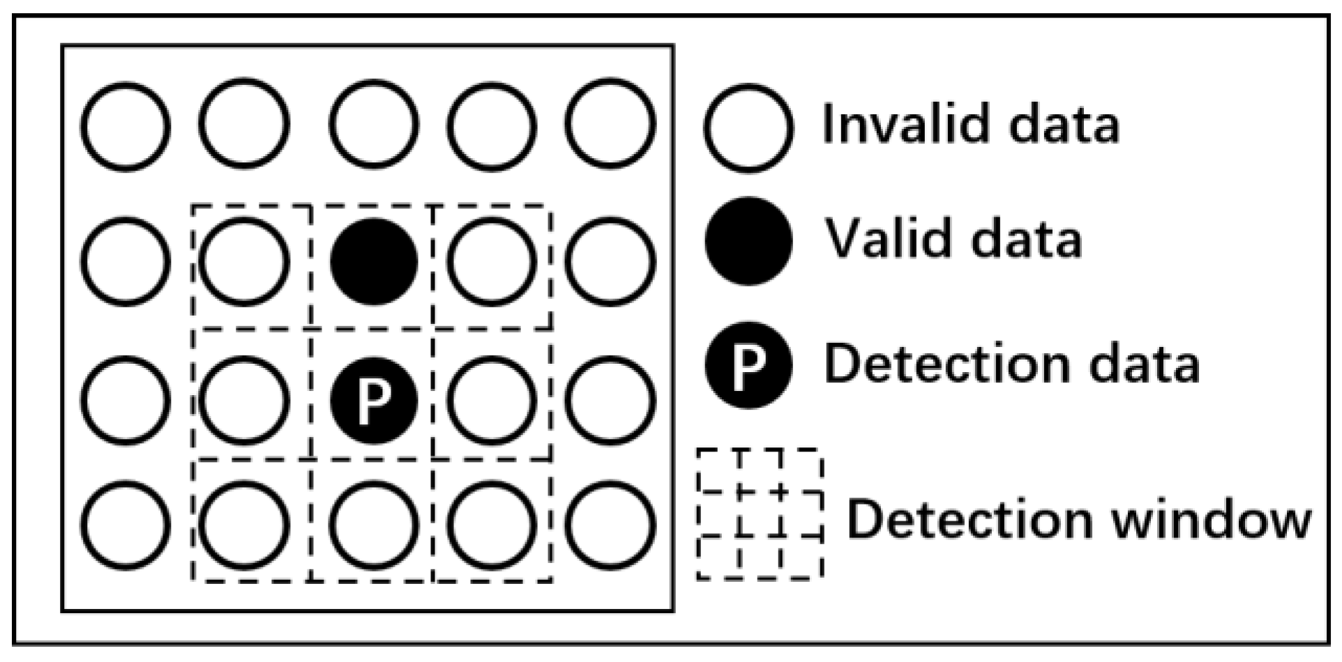
To reduce the influence of noise on the recognition result, it is necessary to remove the isolated points of reflectivity and radial velocity. The method for removing isolated points is to traverse each range bin data, as shown in Figure 1, and count the number of invalid data points around each data point using the $N1$ * $N1$ window. Equation (1) is used to determine whether the data is invalid, and Equation (2) is used to count the number of invalid data around each data point.

$$M=\{\begin{array}{c}1, Data=nan\\ 0, Data\ne nan\end{array}$$

(1)

$$T={\displaystyle \sum }_{i=1}^{N1}{\displaystyle \sum }_{j=1}^{N1}{M}_{i,j}$$

(2)

In Equation (1), the data indicates the reflectivity or the radial velocity, and nan indicates that the data is invalid. When the data is invalid, the value is assigned as 1; when the value is valid, the value is assigned as 0. In Equation (2), $T$ indicates the number of invalid data in the $N1$* $N1$ window around the data point. When $T$ ≥ $T1$, the data point is considered an isolated point and its value is set as invalid.

2.2. Fourier Interpolation Algorithm Improves the Resolution of Reflectivity Products

The azimuth resolution of reflectivity is 1°, and the range resolution of reflectivity is 1 km for the Doppler weather radar in this paper. The azimuth resolution of the radial velocity is 1°, and the range resolution is 0.25 km. Reflectivity and radial velocity should have the same azimuth and range resolution to be combined to complete the identification of the downburst area. As a result, the Fourier interpolation algorithm is used for the radial reflectivity, and the range resolution of radial reflectivity is improved from 1 km to 0.25 km. The essence of the Fourier algorithm [19] is to use Fourier spectrum analysis to obtain the spectral characteristics of the temporal and spatial changes of the reflectivity and further use the spectral characteristics to fit the discrete points of the observation data and then perform resampling. The Fourier interpolation algorithm is used in this paper to perform Fourier interpolation on the reflectivity twice in the radial direction. The radial resolution of reflectivity is doubled with one-time Fourier interpolation. The radial resolution of reflectivity will be improved from 1 km to 0.25 km after two Fourier interpolations.

2.3. Filter

This paper uses the volume scan data of a Doppler weather radar. The radial velocity should be filtered to reduce the noise. After removing isolated points of radial velocity, the value of the range folding is set to an invalid value, and invalid data does not participate in the operation. Then, use the median filter and moving average filter for radial velocity.

• Median filter

Firstly, the median filter selects $N2$ * $N2$ points along the azimuth angle and the radial direction of the point to be processed. Then, the median filter sorts the points (invalid data does not participate in the sorting). Finally, the value of the point to be processed is replaced by the result of the median filter.

2.

Moving average filter

After median filtering, the moving average filter selects $N3$ points along the radial direction of the point to be processed. Then, eliminate invalid values of radial velocity to calculate the average value. Finally, the value of the point to be processed is replaced by the above-average value.

2.4. Two-Dimensional Multi-Channel Algorithm Reduces Velocity Ambiguity in Radial Velocity Products

When the wind speed is large, due to the radial velocity measurement limitation of Doppler radar, velocity ambiguity may appear on the radial velocity. The velocity ambiguity can be identified by discriminating the sudden change of velocity between adjacent points. In 2006, Zhang et al. [20] developed a two-dimensional multi-channel automatic velocity de-aliasing algorithm, which solved the problem of obtaining the initial reference point set. In 2009, Cai et al. [21] made appropriate improvements based on Zhang et al. [20]. To determine the initial reference point set, the two-dimensional channel algorithm first searches for weak wind areas near the velocity line in elevation angle scan data. On three adjacent diameter lines in the wind area, continuity detection and ambiguous correction are performed, followed by two rounds of two-dimensional channel de-aliasing processing in both clockwise and counterclockwise directions. This paper uses a two-dimensional multi-channel algorithm from Cai et al. [21].

2.5. Radial Velocity Interpolation

To improve the accuracy of the downburst recognition result, it is necessary to interpolate the valid-data area in the large radar echo. Equation (3) is used to determine whether the radial velocity data are invalid. Equation (4) is used to count the number of invalid data around each radial velocity data point. Equation (5) is used to calculate the mean value of the valid data in the invalid data point’s $N4$ * $N4$ window.

$$M^{\prime }=\{\begin{array}{c}1, Ve=nan\\ 0, Ve\ne nan\end{array}$$

(3)

$$T^{\prime }={\displaystyle \sum }_{i=1}^{N4}{\displaystyle \sum }_{j=1}^{N4}{M}_{i,j}$$

(4)

$$V{e}^{\prime }=\frac{{{\displaystyle \sum }}_{i=1}^{N4}{{\displaystyle \sum }}_{j=1}^{N4}V{e}_{i,j}}{N4\ast N4-T^{\prime }}$$

(5)

In Equation (3), $Ve$ indicates the radial velocity data, and nan indicates that the data is invalid. When the data is invalid, the value is assigned to 1; when the value is valid, the value is assigned to 0. In Equation (4), $T^{\prime }$ indicates the number of invalid data around the data point in the $N4$ * $N4$ window. In Equation (5), $V{e}^{\prime }$ indicates the average value of the valid data within the $N4$ * $N4$ window of the invalid data point. Each data set is traversed using the radial velocity interpolation method. When $T^{\prime }$ ≤ T2, the value of the invalid data point is assigned to $V{e}^{\prime }$.

3. The Principle of Automatic Identification Algorithm for Downburst Area

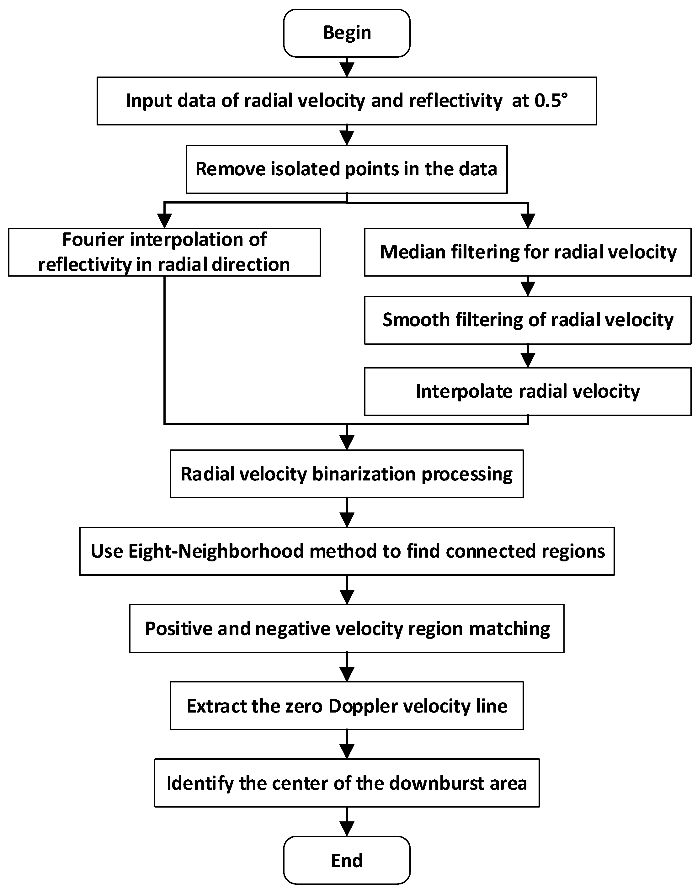
Automatic recognition algorithm for downburst area is that first input the reflectivity and radial velocity of 0.5° elevation, combine the reflectivity and radial velocity threshold to binarize the radial velocity; then use the Eight-Neighborhood method to retrieve the connected areas of positive and negative velocity; then the edge detection of the connected area is performed; then the positive and negative velocity pair matching is performed, and the zero Doppler velocity line between the positive and negative velocity pairs is extracted, and the center identification of the downburst area of the positive and negative velocity is completed.

3.1. Radial Velocity Binarization

To obtain the connected area of positive and negative velocity, the positive and negative velocity in the radial velocity should be distinguished. This is referred to as velocity binarization. Areas with positive radial velocity are classified as positive velocity areas, while areas with negative radial velocity are classified as negative velocity areas.

In the downburst area, there are positive and negative velocity pairs, and the reflectivity is high, generally above 30 dBZ. As a result, the velocity binarization of the downburst area is performed under the aforementioned conditions. If Ve > 0.5 m/s and Ze > T3, then $V{e}_{+}$ = 1; otherwise, $V{e}_{+}$ = 0. If Ve < −0.5 m/s and Ze > T3, then $V{e}_{-}$ = 1; otherwise, $V{e}_{-}$ = 0 (Ze denotes reflectivity, Ve denotes radial velocity, T3 denotes reflectivity threshold, $V{e}_{+}$ denotes positive velocity region grid point, and $V{e}_{-}$ denotes negative velocity region grid point). The data after the binarization of the positive and negative velocity regions are stored separately.

The zero Doppler velocity value of the radial velocity after quality control will fluctuate up and down with the surrounding area data, so the zero Doppler velocity is not suitable as a threshold value to distinguish between positive and negative velocity areas. After many experiments, 0.5 m/s and −0.5 m/s are selected as the threshold to distinguish between positive and negative velocity regions, and the distinguishing effect is more obvious.

3.2. Eight-Neighborhood Method for Matching Positive and Negative Velocity Connected Regions

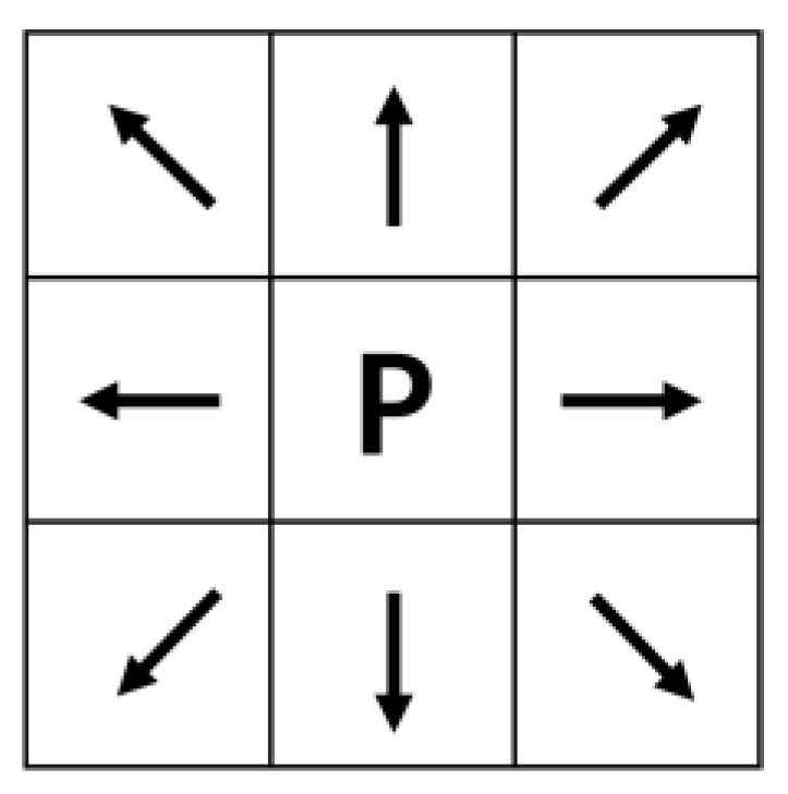
According to the principle of downburst stream recognition, for the binarized velocity image, the Eight-Neighborhood method in the image processing technology (as shown in Figure 2) is used to find the area where the positive and negative velocities are connected along the radial direction. Identify and mark the area where the positive and negative velocities are connected.

To reduce the range of the connected regions of positive and negative velocity and exclude the connected regions of velocity that do not meet the conditions, this paper uses the bwareaopen function [22] to remove the connected regions with pixels less than T4 in the binary image, and generate a new binary image. Then, on the new binary image, perform contour detection. Contour detection determines whether a pixel is a point in a connected region based on the relationship between the selected pixel and its neighboring pixels. If the value of the selected pixel is 1, and the value in the pixel’s Eight-Neighborhood is also 1, the point should be an internal point, and the pixel’s value is overwritten with 0. By traversing the entire image, in turn, all the internal points in the connected region can be removed, and the external contour of the image can be obtained. Record the number of contours in the positive and negative velocity area and the position of the contour centroid, respectively.

Match the identified positive and negative velocity regions. After obtaining the contour of the connected domain of positive and negative velocities, the constrained conditions are used to match the connected regions of positive and negative velocities based on the characteristics of downburst and research on downburst by predecessors Fujita [23] and Wilson [24]. The matching conditions of the positive and negative velocity connected regions are as follows:

• The distance between the positive and negative velocity and the center of mass of the connected area is less than 5 km;
• The number of pixels in the connected area of positive and negative velocity is greater than 10.

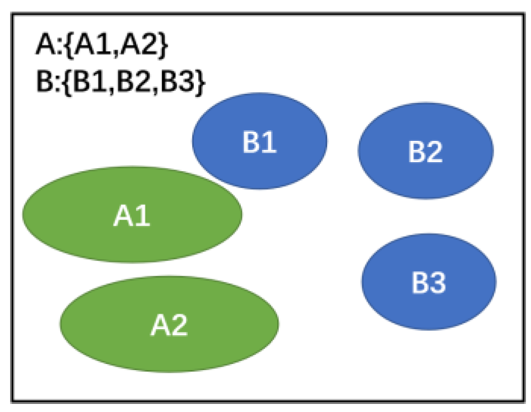
Compare the number of contours in the two groups of positive and negative velocity areas. As shown in Figure 3, define the velocity area with a smaller number of contours as group A, and define the remaining as group B. To match the other velocity zone B in sequence, use a velocity zone A1 from the A group. If velocity zone B1 is the only velocity zone that meets the conditions, it matches velocity zone A1 and is marked. If multiple velocity regions meet the conditions, the centroid distances of the connected regions for multiple velocities should be sorted, and the velocity region B1 with the smallest centroid distance is used as the best matching item for the velocity region A1. After matching all the velocity regions in group A, the matching task of the entire positive and negative velocity pair is completed.

3.3. Zero Doppler Velocity Line Extraction Method

When the positive and negative velocities are matched to the connected regions, one or more pairs of positive and negative velocities will be obtained. To extract the zero Doppler velocity line accurately, the zero Doppler velocity line will be extracted for each pair of positive and negative velocities individually.

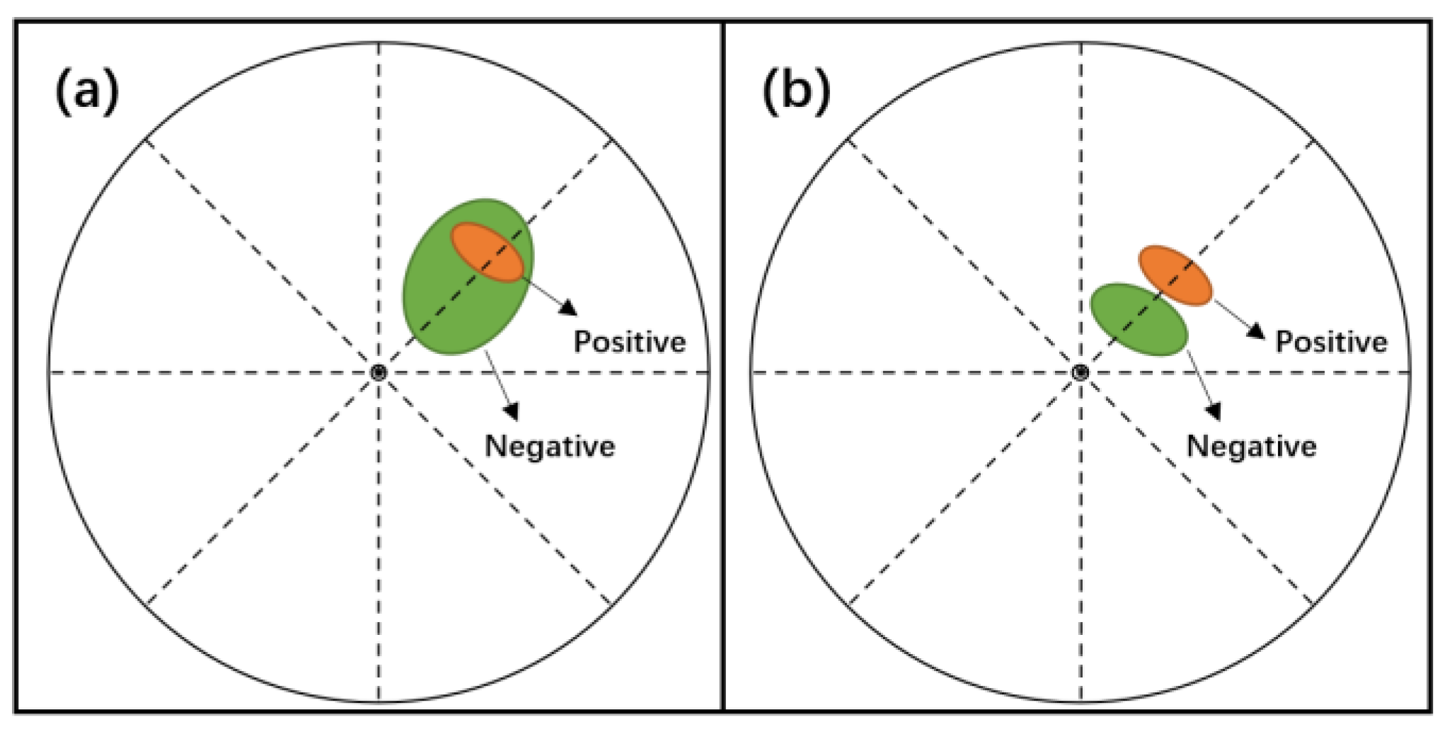
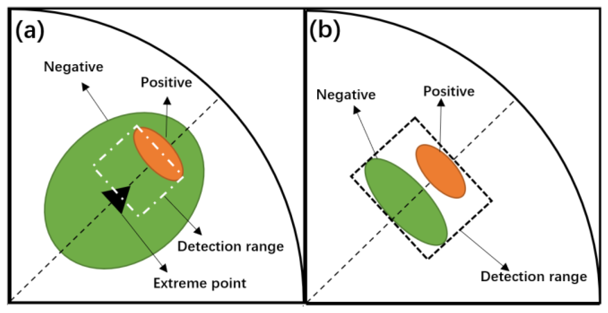
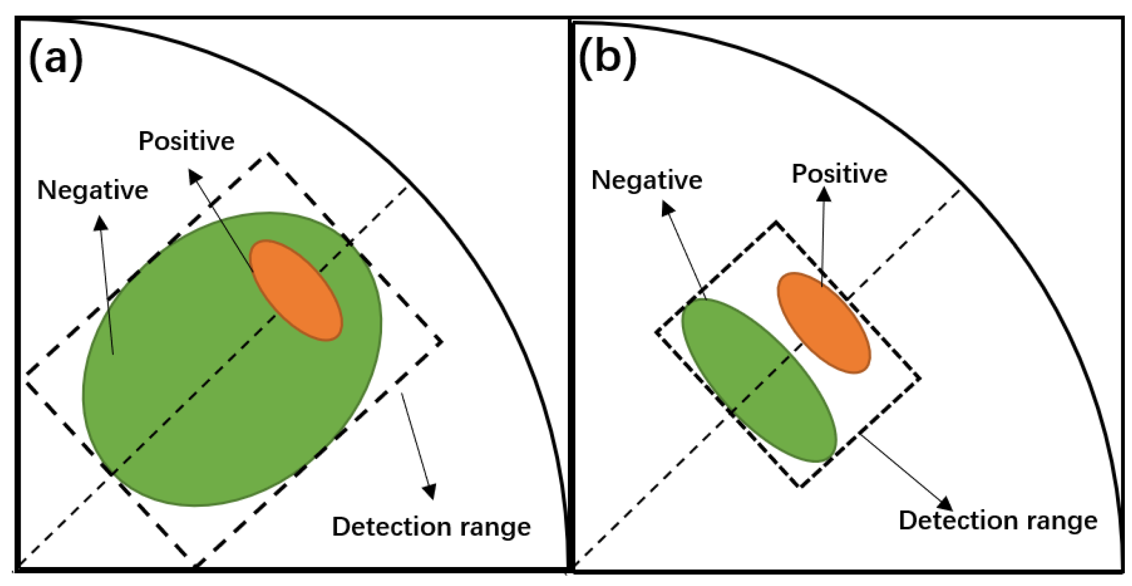
To improve the accuracy of the zero Doppler velocity line recognition, before extracting the zero Doppler velocity line, it is necessary to classify the positive and negative velocity pairs. The positive and negative velocity area is located on both sides of the zero Doppler velocity line, the positive and negative velocity pair is crossed by a radial line, the negative velocity is on the side close to the radar, and the positive velocity is on the side far away from the radar. It is divided into two categories based on the relative position of the detected positive and negative velocity contours. As shown in Figure 4a, the first category is that the contour of one velocity envelops the contour of another velocity. The first category can be described as a large circle that encloses a small circle. As shown in Figure 4b, the second category is that the positive and negative velocity contours are adjacent but not touching.

As shown in Figure 5a, for the first type of velocity pair, the zero Doppler velocity azimuth angle detection range is to determine the maximum and minimum values of the small circle azimuth angle and use them as the detection azimuth range. The mean value of the maximum and minimum values of the small circle’s range bin serves as a limit, and the distance between the extreme points of the large circle serves as another. This ensures that the detected zero Doppler line is located between the extremes of positive and negative velocity. As shown in Figure 5b, for the second type of velocity pair, the maximum azimuth angle and the minimum azimuth angle in the profile of the positive and negative velocity pairs are used as the azimuth angle detection range. The maximum range bin value and the minimum range bin value in the profile of the positive and negative velocity pairs are used as the radial distance detection range.

The first and second types of velocity pairs use the same zero Doppler detection method. The detailed steps are as follows:

• Traverse the radial velocity in the detection range. When the absolute value of the radial velocity ≤ 0.5 m/s, mark this point as a zero Doppler velocity suspected point.
• Within the detection range, use a 3 × 3 window to traverse every suspected point of zero Doppler velocity and record the number of data that satisfy the absolute value of the radial velocity ≤ 0.5 m/s.
• When the total value of the 3 × 3 window of the zero Doppler velocity suspected point meets the condition is ≥2, the zero Doppler velocity suspected point is marked as the zero Doppler velocity point.

After all grid points are traversed, the zero Doppler velocity point set is obtained as the zero Doppler velocity line. If there are multiple pairs of positive and negative velocities, repeat the above step (1) to step (3).

3.4. Recognition Method of Downburst Area Center

When there is downburst weather, the velocity field has a divergent characteristic. Downburst’s basic feature is ground divergence. Due to the interaction of the flow fields, the ground divergence is not necessarily completely symmetrical, which brings certain difficulties to the identification of downbursts.

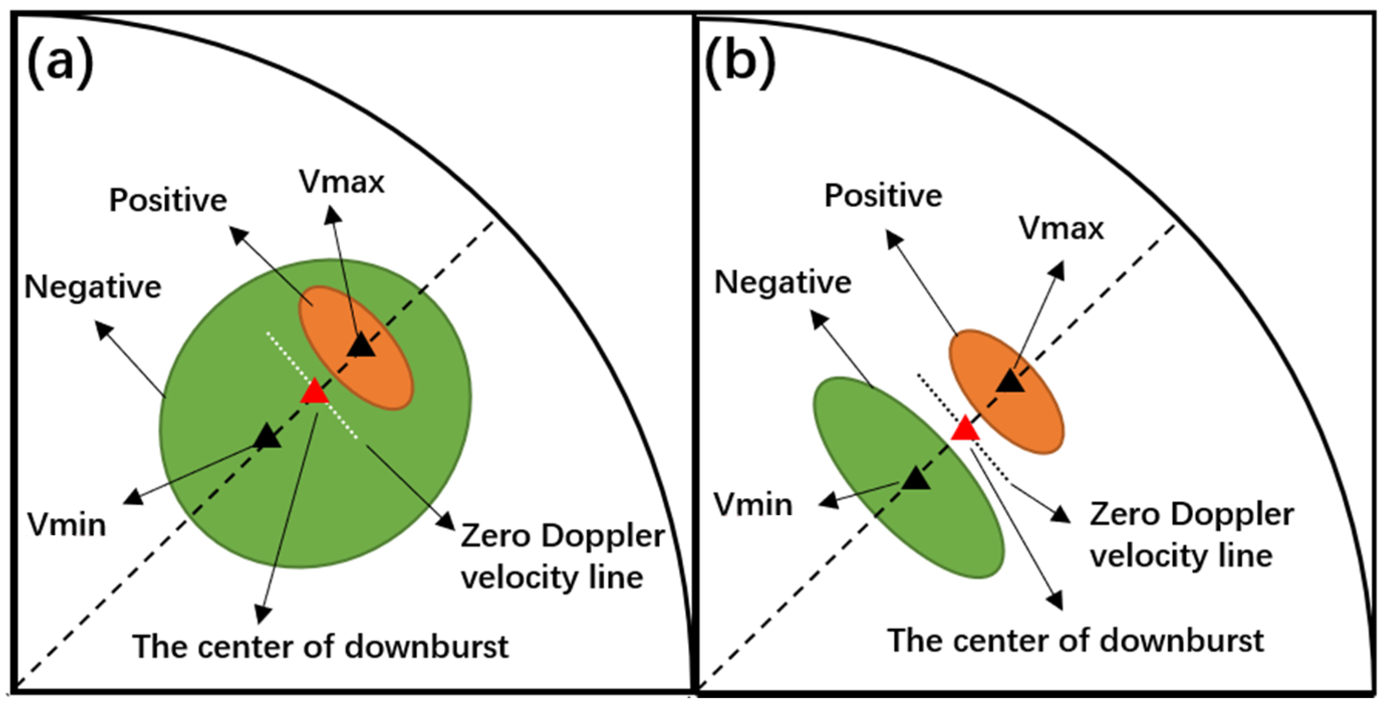
According to the characteristics of the downburst velocity field, it can be obtained that the downburst center is located between the positive and negative velocity extreme points. Then, after extracting the zero Doppler velocity line, the center of the downburst area is identified. The method is as follows:

• As shown in Figure 6, the maximum and minimum values of a pair of positive and negative velocities versus regional azimuth and distance libraries are used as the search range of velocity extremes.

2.

In the search range, find the maximum value of positive velocity and the minimum value of negative velocity, and record the value and coordinates.

3.

Take the absolute value of the maximum value of the positive velocity and the minimum value of the negative velocity. If one of the absolute values is ≥ 10 m/s [25], proceed to step (4); otherwise, the positive and negative velocity have no downburst center.

4.

Calculate the sum of the squares of the distances between all points on the zero Doppler velocity line and the maximum and minimum positive and negative velocity values. As shown in Figure 7, the suspected point at the center of the downburst area is the one where the sum of the squares of the distance is the smallest.

5.

When the reflectivity of the suspected point at the center of the downburst area is greater than 35 dBZ, mark this point as the center point of the downburst area.

6.

If there are multiple pairs of positive and negative velocities, repeat step (1) to step (5).

As shown in Figure 8, it is the flow chart for identifying the downburst area.

4. Case Analysis

To test the actual effect of the macro downburst image recognition algorithm, this paper uses the data of the downburst cases detected by the Doppler radar on 25 July 2006, and 27 June 2009, in Jinan, Shandong Province, to conduct algorithm verification.

4.1. Recognition of Downburst on 25 July 2006

4.1.1. Weather Process Description

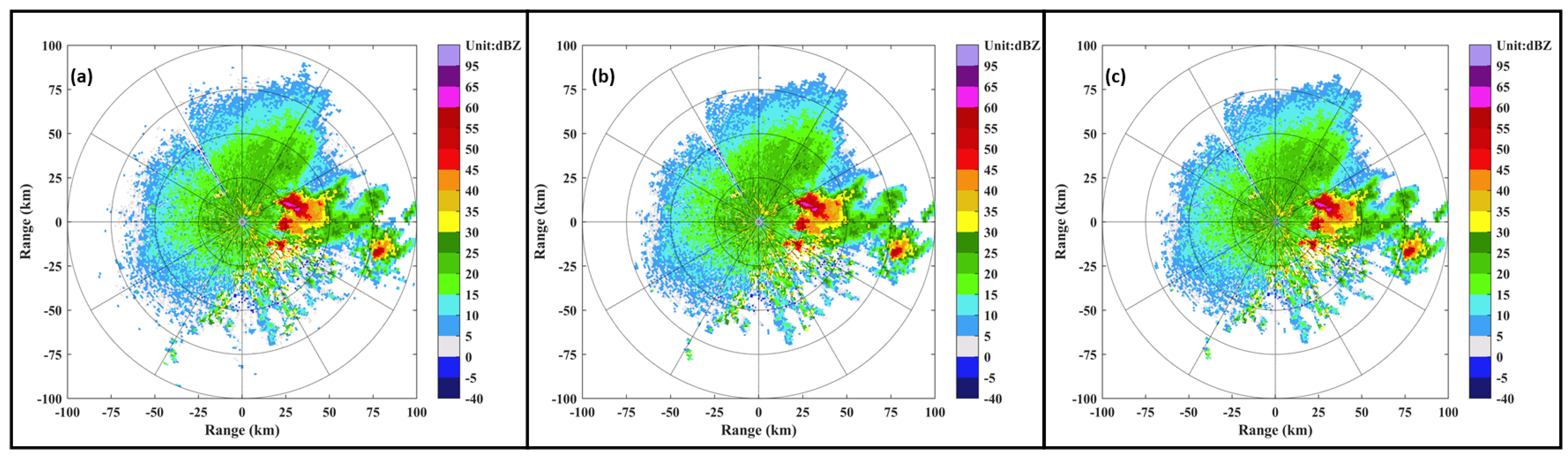
The storm formed at 13:50 (Beijing time, the same below) on 25 July 2006, and dissipated at 17:15. This strong convective weather was caused by the storm monomer E0 from the plane position indicator (PPI) of reflectivity (Figure 9a). During the storm’s mature period, the reflectivity was maintained above 60 dBZ [26].

During the evolution of the storm, the storm moves in the direction of about 70~90° away from the radar, and the middle layer has a positive radial velocity. At 15:19, the radial velocity of the monomer E0 in the hollow (5.5 km) is negative (Figure 9b), indicating that there is a significant rotating updraft inside the monomer. After 15:19, the reflectivity of cyclonic gradually strengthens. At 15:44, the negative minimum radial velocity value is 10~14 m/s, the positive maximum radial velocity value is 20~24 m/s, and the difference between the positive and negative velocities is 30~38 m/s (Figure 9c). At 15:56, the negative minimum radial velocity value is 15~19 m/s, the positive maximum radial velocity value is 20~24 m/s, and the difference between the positive and negative velocities is 35~43 m/s (Figure 9d). At 16:02, the difference between the positive and negative velocities reaches a maximum of about 40~48 m/s. At 16:08, the difference between the positive and negative velocities decreases rapidly, and the negative minimum radial velocity value is 10~14 m/s, the positive maximum radial velocity value is 15~19 m/s, and the difference between the positive and negative velocities is 25~33 m/s (Figure 9e). At 16:21, the negative minimum radial velocity value is 1~4 m/s, the positive maximum radial velocity value is 5~9 m/s, and the difference between the positive and negative velocities is 6~13 m/s (Figure 9f). From 15:19 to 16:02, a cyclonic circulation appeared in the middle of the storm, and the difference between the positive and negative velocities gradually increased. This indicated that the updraft within the storm was also gradually increasing, which contributed to the storm’s strengthening and maintenance.

4.1.2. Recognition of Downburst at 16:02 on 25 July 2006

To improve the accuracy of downburst identification, before downburst identification, data quality control on reflectivity and radial velocity is required.

For quality control of reflectivity, first, remove the isolated points of reflectivity. Figure 10b depicts the outcome of removing the isolated points of reflectivity. Then, the reflectivity is subjected to Fourier interpolation twice along the radial direction, and the result is shown in Figure 10c. After the reflectivity is subjected to radial Fourier radial interpolation twice, the radial resolution is improved from 1 km to 0.25 km. During the processing, the parameters are set as follows: N1 = 3, T1 = 5.

For quality control of radial velocity, first, remove the isolated points of the radial velocity. Figure 11b depicts the outcome of removing the isolated points of radial velocity. Then, apply median filtering to the radial velocity. The result is shown in Figure 11c. Then, the radial velocity is disambiguated, smoothed, and filtered. Figure 11d depicts the outcome. Finally, for radial velocity interpolation, the result is shown in Figure 11e. During the processing, the parameters [27,28,29] are set as follows: N1 = 3, N2 = 3, N3 = 9, N4 = 3, T1 = 5, T2 = 6.

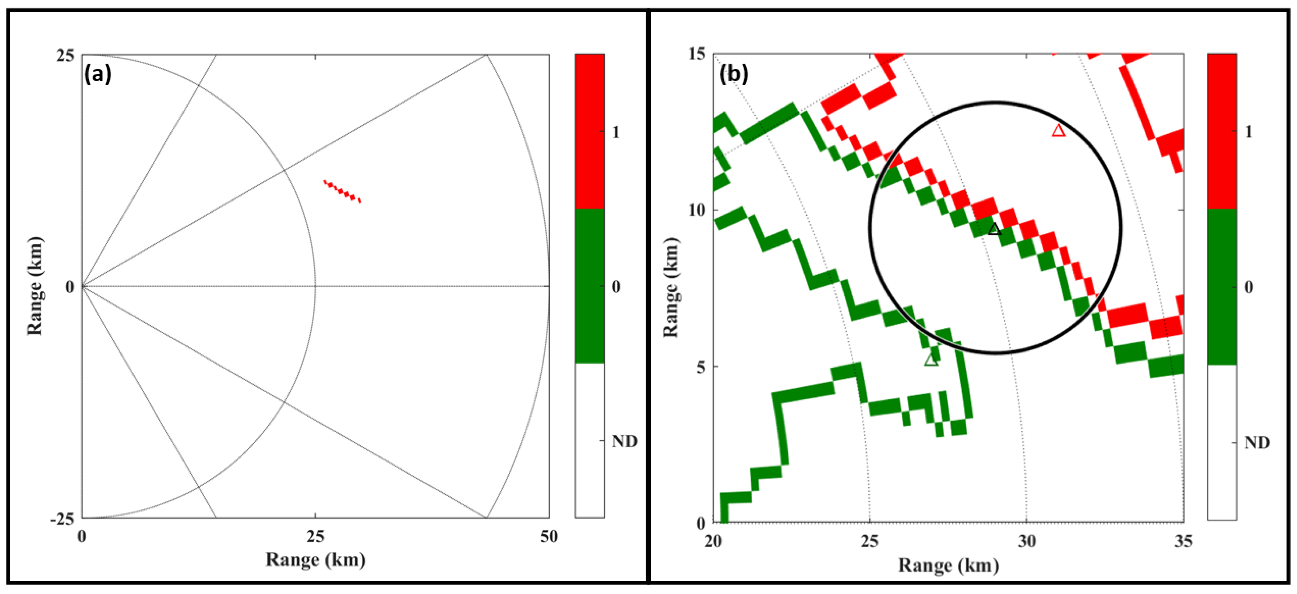
As shown in Figure 12a, the radial velocity is binarized. Then, the edge detection of the binary image is performed, and the result is shown in Figure 12b. The contours of the connected components of positive and negative velocities are matched under constrained conditions after obtaining the contours of the connected components of positive and negative velocities. The pair of positive and negative velocities successfully matched is shown in Figure 12c. During the processing, the parameters are set as follows: T3 = 30 dBZ, T4 = 70.

In the region of successfully matched positive and negative velocity pairs, the zero Doppler velocity line is extracted. Figure 13a depicts the extracted zero Doppler velocity line. Next, locate the downburst’s center between the positive and negative velocity pairs. The upper and lower limits of the search range are the maximum and minimum values of the azimuth of the positive and negative velocity versus the area and the distance library to ensure the accuracy of the recognition of the positive and negative velocity extremes. The red triangle in Figure 13b indicates the position of the maximum positive velocity, and the green triangle indicates the location of the minimum negative velocity. At this point, if the absolute value of any extreme value of the positive and negative velocity is greater than or equal to 10 m/s, then the positive and negative velocity pair has a downburst, and then the downburst center is identified. Finally, the suspected point in the center of the downburst area is determined by the shortest distance between the positive and negative velocity extreme points on the zero Doppler velocity line. When the reflectivity of the suspected point at the center of the downburst area exceeds 35 dBZ, the point is designated as the downburst area’s center point. In Figure 13b, the black triangle represents the downburst center, which is located at 70° tangential to the radar center and 30 km in the radial direction. The black circle represents the downburst range with a radius of 4 km. Symbols in subsequent figures have the same meanings as here.

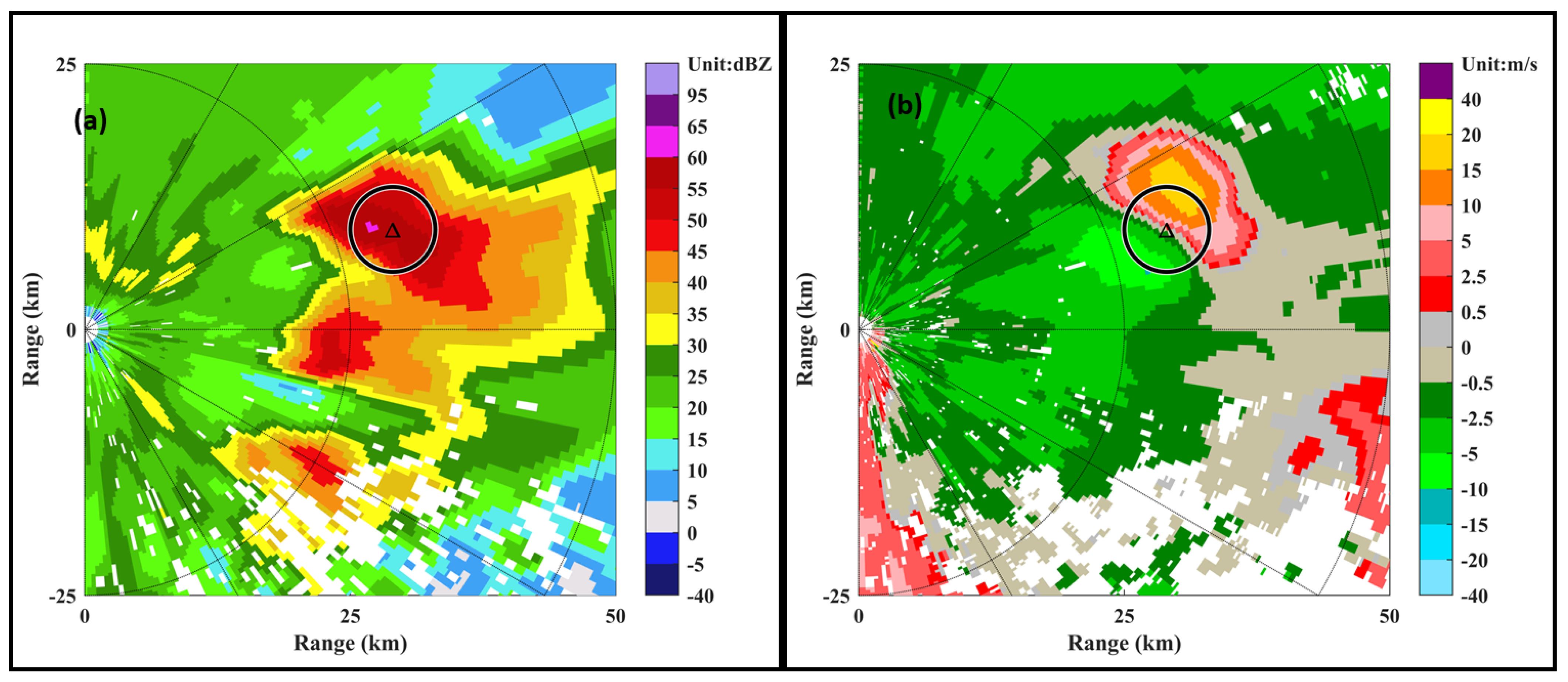
After successfully identifying the area and center of the downburst, the recognition result is mapped on the 0.5° reflectivity and radial velocity PPI, as shown in Figure 14.

4.1.3. Identification of Downburst during This Process

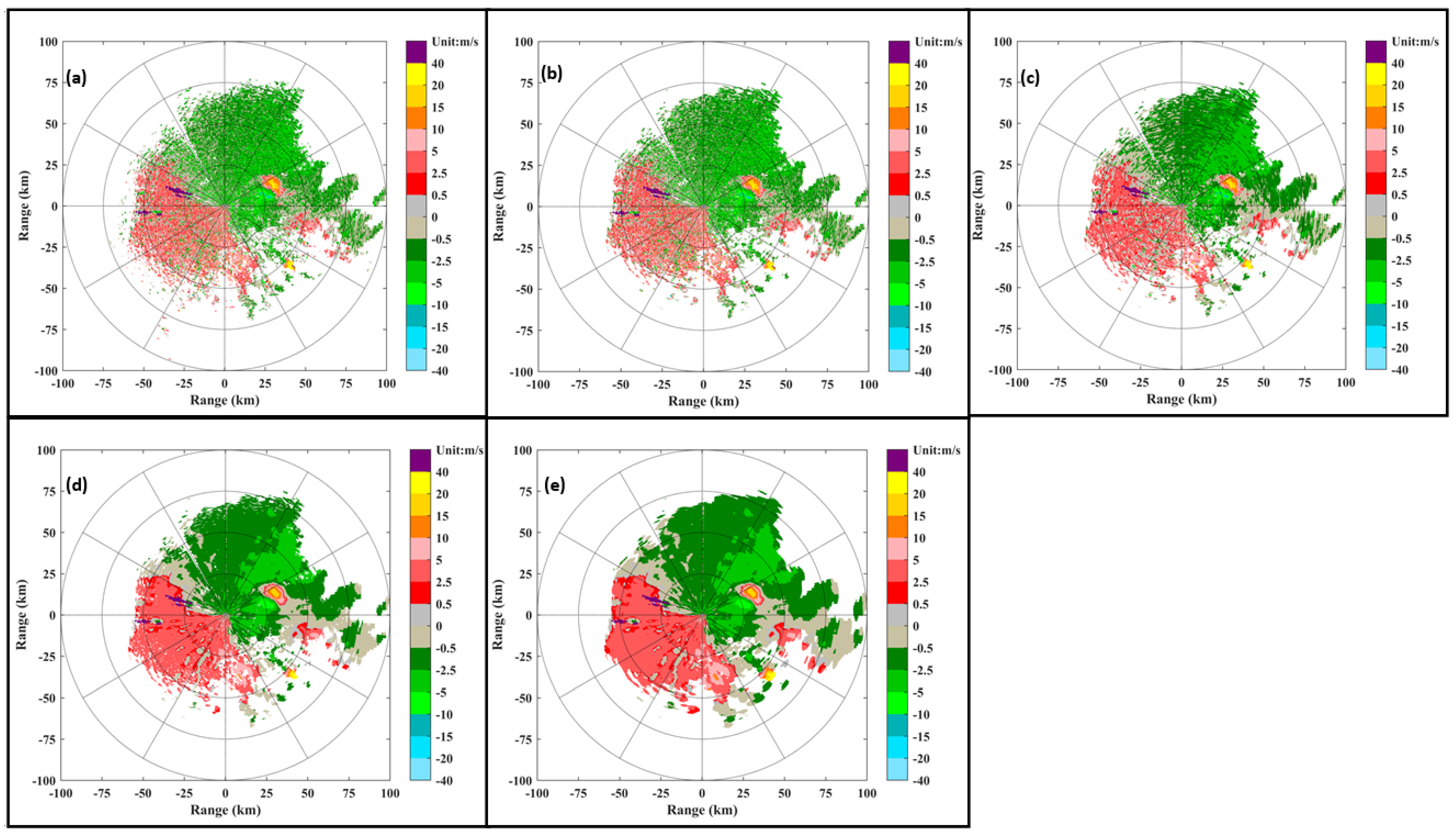
Figure 15a–e is the radial velocity PPI at 0.5° at five moments of the storm. The recognition result of the downburst is that the center of the downburst is represented by a black triangle, and the range of the downburst is represented by a black circle (The radius is 4 km). The storm’s lowest level corresponds to a height of about 0.4 km. The lower level is northeast wind. Figure 15f is the radial velocity PPI after the storm.

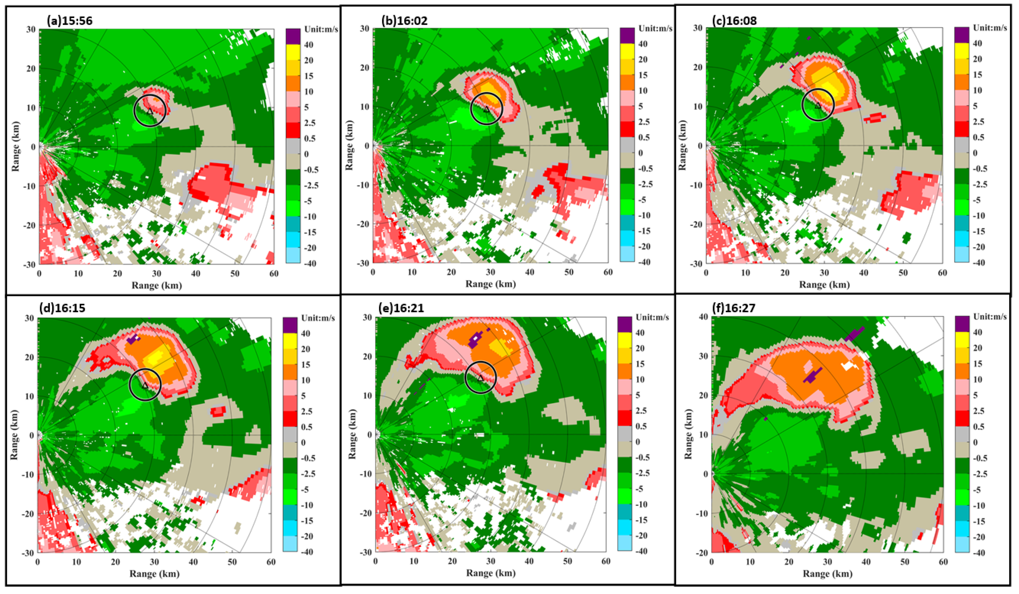
At 15:50, a positive radial velocity appeared in the lower layer of the storm, which is about 1~4 m/s. Then a sinking divergent airflow appeared at the bottom layer, and this divergent airflow became more and more obvious. At 15:56, the maximum value of the positive radial velocity is 5~9 m/s, the minimum value of the negative radial velocity is 15~19 m/s, and the difference between the positive and negative velocities is 20~28 m/s. The downburst center (Figure 15a) is located at 70° tangential to the radar center and 30 km in the radial direction. At 16:02, the maximum value of positive radial velocity is 15~19 m/s, the minimum value of negative radial velocity is 20~26 m/s, and the difference between the positive and negative velocities is 35~45 m/s. The downburst center (Figure 15b) is located at 72° tangential to the radar center and 30 km in the radial direction. At 16:08, the positive radial velocity maximum is 20~26 m/s, the minimum of negative radial velocity is 15~19 m/s, and the difference between the positive and negative velocities is 35~45 m/s. The downburst center (Figure 15c) is located at 72° tangential to the radar center and 30 km in the radial direction. At 16:15, the maximum of the positive radial velocity is 15~26.5 m/s, the minimum of negative radial velocity is 15~23.5 m/s, and the difference between the positive and negative velocities is 30~50 m/s. The downburst center (Figure 15d) is located at 65° tangential to the radar center and 30 km in the radial direction. At 16:21, the absolute value of the radial velocity decreases rapidly, the absolute value of the radial velocity is 15~19 m/s, and the downburst center (Figure 15e) is located at 62° tangential to the radar center and 31 km in the radial direction.

Compared with the monomer trend, the height of the strong center of the monomer has a downward trend from 15:50 to 15:56. From 15:56 to 16:02, the height of the monomer has a significant downward trend, and the radial velocity divergence at the low level gradually strengthens. From 16:02 to 16:15, the height of the strong center drops rapidly. The strong divergence of the lower layer continues until 16:15. The decrease in the height of the monomer’s strong center strengthens the sinking airflow, and the subsequent decrease in the top height and decrease in the strong center intensifies the sinking airflow and produces a torrent of ground blows. According to the disaster investigation [26], the gale lasted more than 10 min, and the disaster area encompassed more than 4 km, which was caused by a macro downburst.

4.2. Recognition of Downbursts on 27 June 2009

4.2.1. Weather Process Description

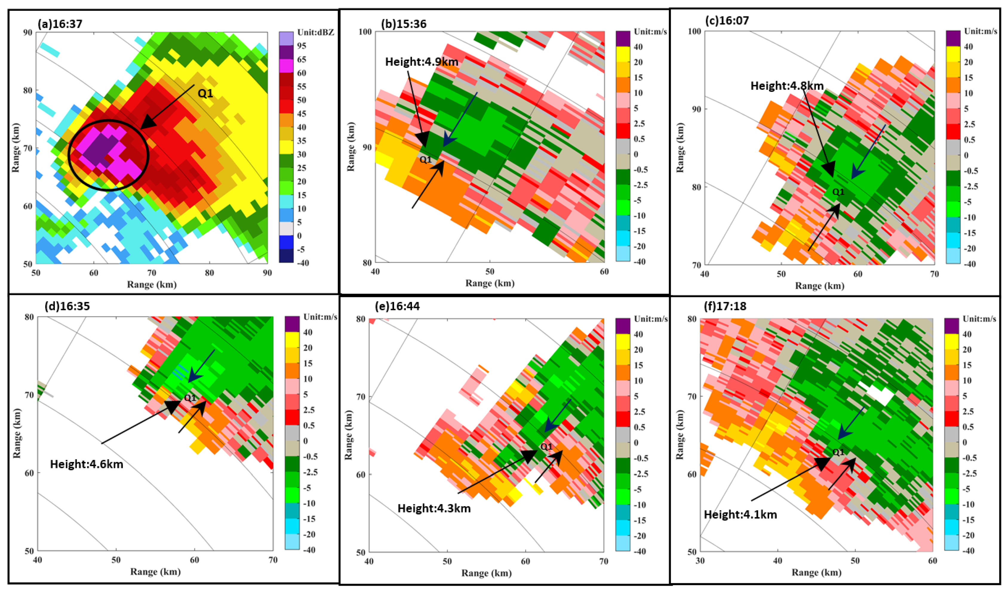
The 0627 storms caused hail and windy weather; they formed at about 14:50 and dissipated at about 17:40, lasting about 3 h. The strong convective weather was caused by the strong storm monomer Q1 (Figure 16a). The peak height of the monomer Q1 was maintained above 10 km during the vigorous phase of the monomer Q1, and the maximum reflectivity was maintained between 60 dBZ and 70 dBZ.

Figure 16b–f shows the radial velocity PPI of 2.4° at five moments of the storm, and the corresponding altitude is between 4 and 5 km. The middle layer of the storm has a radial convergent structure, as shown by the radial velocity diagram in Figure 16b,c. At 15:36, the negative minimum radial velocity value is 5~9 m/s, the positive maximum radial velocity value is 10~14 m/s, and the difference between the positive and negative velocities is 15~23 m/s. At 16:07, the difference between the positive and negative velocities is 15~23 m/s. At 16:13, the storm’s middle layer became a cyclonic convergence, indicating that the updraft had been strengthened. The corresponding strong center height had risen rapidly to more than 10 km, and the cyclonic convergence structure (Figure 16d,e) was maintained until 17:06. The maintenance of this cyclonic convergent structure is conducive to the storm’s development and maintenance so that the storm is maintained at a higher altitude and stronger reflectivity. At 16:25, the negative minimum radial velocity value is 10~14 m/s, the positive maximum radial velocity value is 10~14 m/s, and the difference between the positive and negative velocities is 20~28 m/s (Figure 16d). At 16:44, the difference between the positive and negative velocities is 25~33 m/s (Figure 16e). After 17:06, the cyclonic convergent structure became a radial convergent structure again (Figure 16f) until the storm weakened and died.

4.2.2. Identification of Downburst during This Process

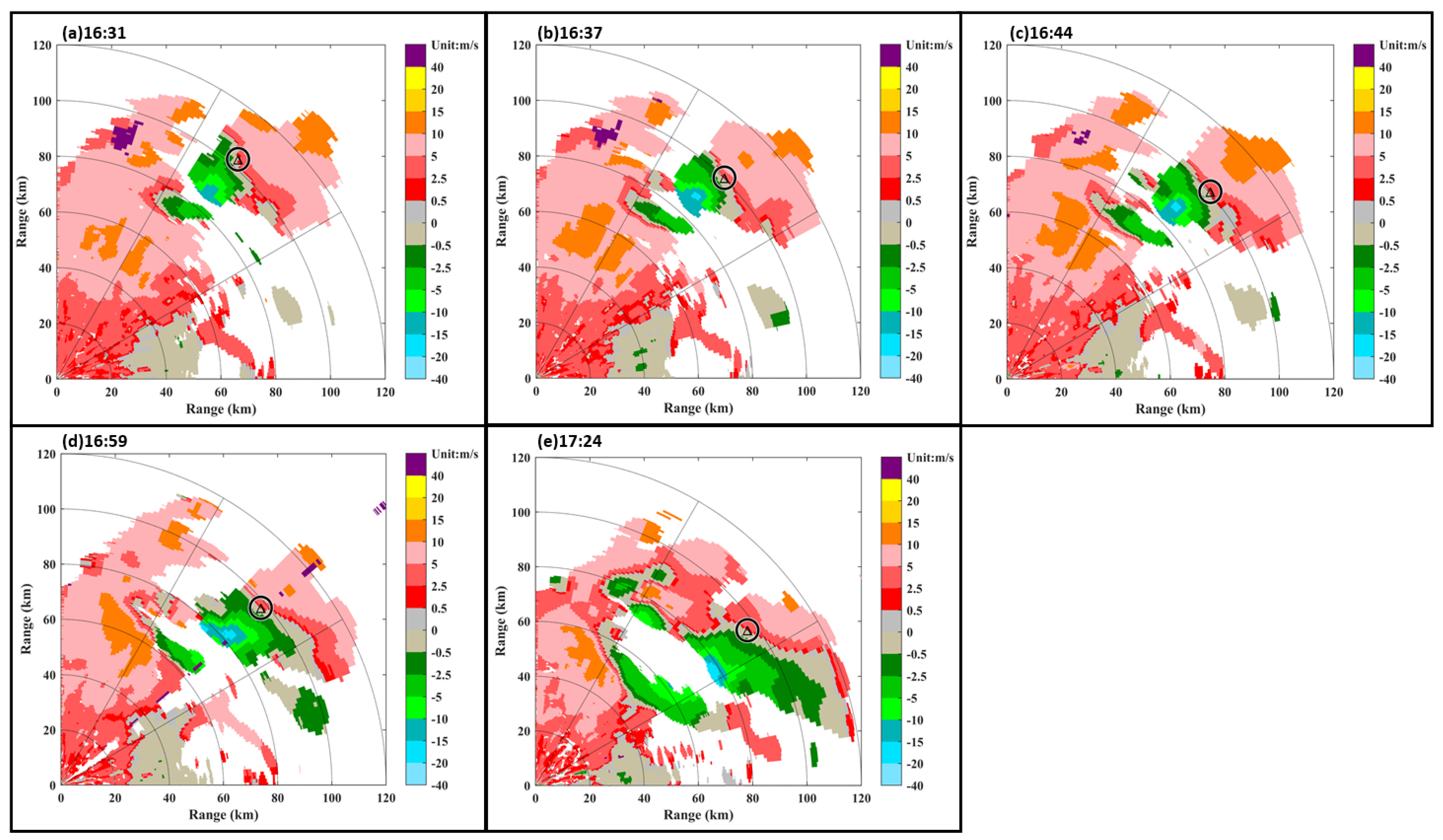
Figure 17a–e is the radial velocity PPI of the 0.5° at five moments of the storm, and the corresponding height is 1~1.3 km. The downburst identification result is the black triangle to indicate the downburst center, and the black circle indicates the range of the downburst.

At 16:31, the negative radial velocity is 15~19 m/s, and the downburst center (Figure 17a) is located at 40° tangential to the radar center and 105 km in the radial direction. At 16:37, the negative radial velocity is 20~24 m/s, and the downburst center (Figure 17b) is located at 43° tangential to the radar center and 100 km in the radial direction. At 16:44, the negative radial velocity continues to decrease, and the velocity blur appears, with a magnitude of 28~34 m/s. The downburst center (Figure 17c) is located at 46° tangential to the radar center and 101 km in the radial direction. At 16:59, the downburst center (Figure 17d) is located at 48° tangential to the radar center and 97 km in the radial direction. At 17:12, the velocity blur phenomenon continues until 17:18, and the velocity is basically maintained at 28~34 m/s. At 17:24, the radial velocity blur disappears, and the negative radial velocity value is 20~24 m/s. The downburst center (Figure 17e) was located at 54° tangential to the radar center and 97 km in the radial direction, which the cell gradually disappeared. Compared with the monomer trend, the height of the strong center of the monomer drops rapidly from 10.2 km to 4.4 km at 16:19~16:31. At 16:31, the absolute value of the radial velocity of the low layer increases rapidly, and then the absolute value of the lower radial velocity continues to increase. The peak height of the monomer dropped rapidly at 16:59, so the absolute value of the radial velocity of the lower layer was continuously maintained to 17:18.

The height detected by the Jinan SA radar is 1.1~1.3 km and is not a reflection of ground velocity. The wind velocity recorded by the mesoscale observation station in Jianglou Town on the ground is 26 m/s at 17:00~17:10. The extreme value was 30 m/s at 17:10~17:20, and the gusts reached 10~11 levels. Due to the density of mesoscale observatories, the live records were small before 17:00. The low-level radial velocity map shows a large value area between 28 m/s and 34 m/s, which corresponds to 10~11 gusts on the ground. According to the on-site disaster investigation [26], the destructive gale lasted more than 30 min, and the distance of the destructive gale was more than 20 km (Figure 17e), indicating a macro storm. At 16:25, the height of the strong center of the monomer began to drop, and the lower level appeared with a large radial velocity at 16:44.

The radial velocity convergence structure of the monolithic mesosphere changed to a cyclonic convergence structure. This cyclonic convergence structure strengthens the updraft and facilitates the development and maintenance of storms. This allows storms to remain at higher altitudes and higher intensities, thus making them prone to extreme catastrophic weather. The height drop of the storm’s strong center stimulated sinking airflow, causing a large radial velocity divergence in the storm’s lower layers. The storm’s decreasing top height strengthened the sinking airflow even more, resulting in extremely destructive windy weather.

4.3. Algorithm Comparison

Both 10 m/s and −10 m/s are selected as the threshold to distinguish between positive and negative velocity regions, and the reflectivity threshold for radial velocity binarization is 20 dBZ in the algorithm proposed by Du [15]. When affected by the environmental wind field, the absolute value of some velocity maximum values does not reach 10 m/s (Figure 18a), which will lead to missed detections in the positive and negative velocity regions (Figure 18c,d). Both 0.5 m/s and −0.5 m/s are selected as the threshold to distinguish between positive and negative velocity regions, and 30 dBZ is selected as the reflectivity threshold in this paper. Combined with the features of high reflectivity (Figure 18b) in the downburst region, the region with large velocity can be effectively identified (Figure 18e,f). The case shows that the change of the threshold improves the detection probability of positive and negative velocity regions.

The positive and negative velocity difference of 35 m/s is one of the constraints when determining a downburst using the algorithm proposed by Du [15]. Under the macro downburst, the velocity is more affected by the environmental wind field, and the positive and negative velocity difference of 35 m/s is not suitable as the condition for determining the macro downburst. In order to expand the application range of the downburst identification algorithm, this paper does not add the condition of positive and negative velocity differences in the constraint conditions. Since the cases in this paper belong to the macro downburst, the algorithm produced by Du was used, and the downburst was not successfully identified.

5. Conclusions

Based on the algorithm proposed by Du [15], this paper improves the algorithm for downburst region identification based on image processing using a single Doppler weather radar low-level radial velocity and reflectivity data for macro downburst. First, the velocity threshold of radial velocity binarization is reduced from 10 m/s to 0.5 m/s, and the reflectivity threshold for radial velocity binarization in this paper is increased from 20 dBZ to 30 dBZ. Section 4.3 shows that the change of the threshold improves the detection probability of positive and negative velocity regions. Second, a new algorithm is added to identify the center of the downburst region. The extraction method of the zero Doppler velocity line is proposed in the algorithm of downburst region center identification. The cases of Section 4.1 and Section 4.2 shows that the algorithm can identify the center of the downburst region.

To mitigate the impact of data quality on downburst identification, this paper firstly conducts data quality control on the reflectivity and radial velocity. Performs isolated point removal and Fourier interpolation on the reflectivity data; performs isolated point removal, filtering processing, disambiguates velocity and interpolation processing on the radial velocity. After performing data quality control, combine the reflectivity and the radial velocity threshold to binarize the radial velocity; then, using the Eight-Neighborhood method, retrieve the positive and negative velocity connected areas; and finally, perform edge detection on the connected areas. Then, match the positive and negative velocity pairs and extract the zero Doppler velocity line between them. Complete the downburst identification by combining the downburst velocity field characteristics. This algorithm is used to identify the Doppler radar data of two downbursts in Jinan, Shandong. The results show that the algorithm can identify the center of the downburst, and it has a good identification effect on the center of the downburst with asymmetric divergence due to the influence of the environmental wind field. In addition, the algorithm has limitations for the downburst identification of multi-cell storms.

References

- Fujita, T.T. Tornadoes and Downbursts in the Context of Generalized Planetary Scales. J. Atmos. Sci. 1981, 38, 1511–1534. [Google Scholar] [CrossRef] [Green Version]
- Fujita, T.T.; Satellite and Mesometeorology Research Project. The Downburst: Microburst and Macroburst: Report of Projects NIMROD and JAWS; Satellite and Mesometeorology Research Project, Department of the Geophysical Sciences, University of Chicago: Chicago, IL, USA, 1985; 122p. [Google Scholar]
- Xiao, Y.J.; Wang, J.; Wang, Z.B.; Leng, L.; Fu, Z.K. A Downburst Nowcasting Method Based on Observations of S-Band New Generation Weather Radar. Meteorol. Mon. 2021, 47, 919–931. [Google Scholar]
- Merritt, M.W. Automated Detection of Microburst Windshear for Terminal Doppler Weather Radar. Proc. SPIE 1988, 846, 61–69. [Google Scholar]
- Roberts, R.D.; Wilson, J.W. A Proposed Microburst Nowcasting Procedure Using Single-Doppler Radar. J. Appl. Meteorol. 1989, 28, 285–303. [Google Scholar] [CrossRef] [Green Version]
- Wolfson, M.M.; Delanoy, R.L.; Forman, B.E.; Hallowell, R.G.; Pawlak, M.L.; Smith, P.D. Automated Microburst Wind-Shear Prediction. Linc. Lab. J. 1994, 7, 399–426. [Google Scholar]
- Smith, T.M.; Elmore, K.L.; Dulin, S.A. A Damaging Downburst Prediction and Detection Algorithm for the WSR-88D. Weather Forecast. 2004, 19, 240–250. [Google Scholar] [CrossRef]
- Tuttle, J.D.; Bringi, V.N.; Orville, H.D.; Kopp, F.J. Multiparameter Radar Study of a Microburst: Comparison with Model Results. J. Atmos. Sci. 1989, 46, 601–620. [Google Scholar] [CrossRef] [Green Version]
- Herzegh, P.H.; Jameson, A.R. Observing Precipitation through Dual-Polarization Radar Measurements. Bull. Am. Meteorol. Soc. 1992, 73, 1365–1376. [Google Scholar] [CrossRef] [Green Version]
- Kumjian, M.R.; Khain, A.P.; Benmoshe, N.; Ilotoviz, E.; Ryzhkov, A.V.; Phillips, V.T.J. The Anatomy and Physics of ZDR Columns: Investigating a Polarimetric Radar Signature with a Spectral Bin Microphysical Model. J. Appl. Meteorol. Climatol. 2014, 53, 1820–1843. [Google Scholar] [CrossRef]
- Kuster, C.M.; Bowers, B.R.; Carlin, J.T.; Schuur, T.J.; Brogden, J.W.; Toomey, R.; Dean, A. Using KDP Cores as a Downburst Precursor Signature. Weather Forecast. 2021, 36, 1183–1198. [Google Scholar] [CrossRef]
- Yu, X.D.; Zhang, A.M.; Zheng, Y.Y.; Fang, C.; Zhu, H.F.; Wu, L.L. Doppler Radar Analysis on a Series of Downburst Events. J. Appl. Meteorol. Sci. 2006, 17, 385–393. [Google Scholar]
- Zhao, D.Y.; Bai, J. Review of Researches on Identification and Warning of Downbursts with Doppler Radar. Meteorol. Sci. Technol. 2007, 35, 631–636. [Google Scholar]
- Tao, L.; Dai, J.H. Research on Automatic Detection Algorithm of Downburst. Plateau Meteorol. 2011, 30, 784–797. [Google Scholar]
- Du, M.Y.; Xiao, Y.J.; Wu, T. Identification of Downbursts Based on WSR-88D Doppler Weather Radar Images. Meteorol. Sci. Technol. 2015, 43, 368–372. [Google Scholar]
- Zhao, Z.Y. A Forecast Method of Downburst Based on Doppler Weather Radar. Ph.D. Thesis, Tianjin University, Tianjin, China, 2018. [Google Scholar]
- Sun, J.; Xiao, Y.J.; Leng, L. Damaging downbursts warning algorithm using the Doppler weather radar scanning data. J. Nat. Disasters 2019, 28, 118–126. [Google Scholar]
- Wang, X.; Min, J.Z.; Zhang, L.X.; Ding, L.D.; Cai, S.X. Method of downburst warning based on radar data extrapolation and feature recognition. J. Meteorol. Sci. 2019, 39, 377–385. [Google Scholar]
- Jiao, P.C.; Wang, Z.H.; Chu, C.G.; Han, J.; Zhang, S.; Zhu, Y.Q. An interpolation method for weather radar data based on Fourier spectrum analysis. Plateau Meteorol. 2016, 35, 1683–1693. [Google Scholar]
- Zhang, J.; Wang, S. An Automated 2D Multipass Doppler Radar Velocity Dealiasing Scheme. J. Atmos. Ocean. Technol. 2006, 23, 1239–1248. [Google Scholar] [CrossRef]
- Cai, Q.; Yan, Q. Application study of automated 2D multipass Doppler radar velocity dealiasing scheme. J. Meteorol. Sci. 2009, 29, 625–632. [Google Scholar]
- The Documentation of Bwareaopen Is about Removing Small Objects from Binary Image. Available online: https://ww2.mathworks.cn/help/images/ref/bwareaopen.html?searchHighlight=bwareaopen&s_tid=srchtitle_bwareaopen_1 (accessed on 1 December 2021).
- Fujita, T.T. Objectives, operations, and results of Project NIMROD. In Proceedings of the 11th Conference on Severe Local Storms of the American Meteorological Society, Kansas City, MO, USA, 2–5 October 1979; pp. 259–266. [Google Scholar]
- Wilson, J.W.; Schreiber, W.E. Initiation of Convective Storms at Radar-Observed Boundary-Layer Convergence Lines. Mon. Weather Rev. 1986, 114, 2516–2536. [Google Scholar] [CrossRef] [Green Version]
- Wilson, J.W.; Roberts, R.D.; Kessinger, C.; Mccarthy, J. Microburst Wind Structure and Evaluation of Doppler Radar for Airport Wind Shear Detection. J. Clim. Appl. Meteorol. 1984, 23, 898–915. [Google Scholar] [CrossRef] [Green Version]
- Diao, X.G.; Zhao, Z.D.; Gao, H.J.; Jiang, P. Doppler Radar Echo Features of Three Downbursts. J. Meteorol. Mon. 2011, 37, 522–531. [Google Scholar]
- Ayindir, C.B. A novel nonlinear frequency modulated chirp signal for synthetic aperture radar and sonar imaging. J. Nav. Sci. Eng. 2015, 11, 68–81. [Google Scholar]
- Bayindir, C.; Frost, J.D.; Barnes, C.F. Assessment and Enhancement of SAR Noncoherent Change Detection of Sea-Surface Oil Spills. IEEE J. Ocean. Eng. 2017, 43, 211–220. [Google Scholar] [CrossRef]
- Zhuang, H.; Fan, H.; Deng, K.; Yu, Y. An improved neighborhood-based ratio approach for change detection in SAR images. Eur. J. Remote Sens. 2018, 51, 723–738. [Google Scholar] [CrossRef] [Green Version]
Figure 1.
Schematic of the isolated points detection.
Figure 2.
Schematic of the Eight-Neighborhood method. P is the distance database to be queried. The eight arrows represent the eight neighborhoods of P.
Figure 3.
Schematic of positive and negative velocity zone matching. The group A is the velocity area with a smaller number of contours. The group B is the velocity area with a bigger number of contours.
Figure 4.
Types of positive and negative velocity pairs. (a) A large circle encloses a small circle, and (b) the two circles are adjacent.
Figure 5.
Detection range of the zero Doppler velocity line. (a) Detection range of the zero Doppler velocity line with large and small circles; (b) Detection range of the zero Doppler velocity line with two adjacent circles.
Figure 6.
Range of radial velocity extreme value retrieval. (a) Retrieval range of radial velocity extreme value of large and small circles; (b) Retrieval range of radial velocity extreme value of two adjacent circles.
Figure 7.
Schematic of identifying the center of the downburst area. (a) Schematic of the recognition center of large and small circles; (b) Schematic of the recognition center of two adjacent circles.
Figure 8.
Flow chart of downburst area recognition algorithm.
Figure 9.
Radar echoes from Jinan, Shandong on 25 July 2006. (a) 16:15 is the reflectivity PPI at an elevation angle of 0.5°; (b) 15:19, (c) 15:44, (d) 15:56, (e) 16:08, and (f) 16:21 are radial velocity PPI at 9.9°.
Figure 10.
Reflectivity quality control results at 0.5°. (a) Original data, (b) removed isolated points, and (c) quadratic Fourier interpolation.
Figure 11.
Quality control results of 0.5° radial velocity. (a) Original data, (b) removed isolated points, (c) median filter result, (d) smooth filter result, and (e) interpolation result.
Figure 12.
Eight-Neighborhood method positive and negative velocity connected region matching. (a) Radial velocity binarization, (b) Eight-Neighborhood method edge detection, and (c) positive and negative velocity pair matching results. In the figure, red and green indicate positive and negative velocities.
Figure 13.
Extraction of zero Doppler velocity line and identification of downburst center. (a) Extraction result of zero Doppler velocity line and (b) recognition result of downburst center. In Figure 13b, the red outline represents the positive velocity area, and green outline represents the negative velocity area; the red triangle represents the maximum value of the positive velocity area, and green triangle represents the minimum value of the negative velocity; the black triangle represents the center of the downburst, and black circle indicates the range of the downburst, while the radius of the circle is 4 km.
Figure 14.
Recognition result of the downburst area and center. (a) Downburst area as well as center position on reflectivity PPI, and (b) downburst area and center position on radial velocity PPI.
Figure 15.
Radar echoes from Jinan, Shandong on 25 July 2006. (a) 15:56, (b) 16:02, (c) 16:08, (d) 16:15, (e) 16:21, and (f) 16:27 is the radial velocity PPI at an elevation of 0.5°. The black triangle represents the center of the downburst, and black circle represents the range of the downburst.
Figure 16.
Radar echoes from Jinan, Shandong on 27 June 2009. (a) 16:37 is the reflectivity PPI at an elevation angle of 0.5°; (b) 15:36, (c) 16:07, (d) 16:25, (e) 16:44, and (f) 17:18 are radial velocity PPI at 2.4° elevation.
Figure 17.
Radar echoes from Jinan, Shandong on 27 June 2009. (a) 16:31, (b) 16:37, (c) 16:44, (d) 16:59, and (e) 17:24 are the radial velocity PPI at an elevation angle of 0.5°. The black triangle indicates the center of the downburst, and black circle indicates the range of the downburst.
Figure 18.
Radar echoes at an elevation angle of 0.5° from Jinan, Shandong, on 27 June 2009, 16:31. (a) The PPI of radial velocity, (b) the PPI of reflectivity, (c) radial velocity binarization using the Du’s algorithm, (d) Eight-Neighborhood method edge detection using the Du’s algorithm, (f) radial velocity binarization using the algorithm in this paper, and (e) Eight-Neighborhood method edge detection using the algorithm in this paper. In (c–f), the red outline represents the positive velocity area, and green outline represents the negative velocity area.
Publisher’s Note: MDPI stays neutral with regard to jurisdictional claims in published maps and institutional affiliations. |
© 2022 by the authors. Licensee MDPI, Basel, Switzerland. This article is an open access article distributed under the terms and conditions of the Creative Commons Attribution (CC BY) license (https://creativecommons.org/licenses/by/4.0/).
Share and Cite
MDPI and ACS Style
Wang, X.; Wang, H.; He, J.; Shi, Z.; Xie, C. Automated Recognition of Macro Downburst Using Doppler Weather Radar. Atmosphere 2022, 13, 672. https://0-doi-org.brum.beds.ac.uk/10.3390/atmos13050672
AMA Style
Wang X, Wang H, He J, Shi Z, Xie C. Automated Recognition of Macro Downburst Using Doppler Weather Radar. Atmosphere. 2022; 13(5):672. https://0-doi-org.brum.beds.ac.uk/10.3390/atmos13050672
Chicago/Turabian StyleWang, Xu, Hailong Wang, Jianxin He, Zhao Shi, and Chenghua Xie. 2022. "Automated Recognition of Macro Downburst Using Doppler Weather Radar" Atmosphere 13, no. 5: 672. https://0-doi-org.brum.beds.ac.uk/10.3390/atmos13050672
Note that from the first issue of 2016, this journal uses article numbers instead of page numbers. See further details here.