
Density Estimation of Fog in Image Based on Dark Channel Prior


College of Science, Beijing Forestry University, Beijing 100083, China
*
Author to whom correspondence should be addressed.
Atmosphere 2022, 13(5), 710; https://0-doi-org.brum.beds.ac.uk/10.3390/atmos13050710
Submission received: 6 March 2022
/
Revised: 25 April 2022
/
Accepted: 27 April 2022
/
Published: 29 April 2022
(This article belongs to the Section Atmospheric Techniques, Instruments, and Modeling)
Abstract
:This paper proposes a method and an original index for the estimation of fog density using images or videos. The proposed method had the advantages of convenient operation and low costs for applications in automatic driving and environmental monitoring. The index was constructed based on a dark channel map and the pseudo-edge details of the foggy image. The effectiveness of the fog density index was demonstrated and validated through experiments on the two existing open datasets. The experimental results showed that the presented index could correctly estimate the fog density of images: (1) the estimated fog density value was consistent with the corresponding label in the Color Hazy Image Database (CHIC) in terms of rank order; (2) the estimated fog density level was consistent with the corresponding label in the Cityscapes database and the accuracy reached as high as 0.9812; (3) the proposed index could be used to evaluate the performance of a video defogging algorithm in terms of residual fog.
1. Introduction
Fog or haze in images and videos leads to low visibility and thus, causes major problems in transportation and computer vision applications. Under poor visibility conditions, road traffic accidents often increase greatly. In order to ensure people’s safety whilst traveling, it is necessary for the relevant authorities to make the decision of whether or not to close highways, cancel flights, etc. However, a reliable decision requires an accurate estimation of fog density and images and videos that are taken during reduced visibility conditions are often characterized by blurred details, faded color, lower contrast and overall poor visibility and thus, degrade the performance of outdoor vision systems, such as object recognition, segmentation and remote sensing. In order to accurately detect and process extracted features for computer vision applications, image defogging is an imperative preprocessing step. However, the fog-relevant features closely correlate with the perception of fog density within the image [1], so it is necessary to estimate the fog density in order to select the most appropriate defogging methods. As a result, the estimation of fog density is critical and has a wide range of applications. The definition of fog and the division standard of fog density levels are somewhat different within the fields of physics and meteorology [2]. In terms of measuring methods, fog levels can be estimated using subjective human judgment or measured using instruments, such as a smoke density tester or an optical fog sensor [3]. For most people, foggy weather is often simply divided into three levels, according to visibility: shallow fog, moderate fog and dense fog [4]. According to Koschmieder’s law, horizontal visibility can be estimated simply using the atmospheric extinction coefficient, which is highly relative to the daytime fog density [5,6]. The visibility is then measurable using instruments such as a “visiometer”. Therefore, in meteorology, atmospheric horizontal visibility is usually used to judge fog density levels [5].
Fog density estimation is not just a subjective visual evaluation with the naked eye, but is rather an objective estimation that is based on facts and measurements. In recent years, image-based fog density estimation methods have received an increasing amount of attention [1]. A representative method is the Fog Aware Density Evaluator (FADE) algorithm [7], which is based on the model of NSS (Natural Scene Statistics) and fog-aware statistical features. A pixel-based fog density estimation algorithm was proposed in [8], which is based on two priors and is constructed in the HSV space. Mori et al. [9] proposed a fog density estimation method that uses in-vehicle camera images and millimeter wave (mmW) radar data [9]. This method estimates fog density by evaluating the visibility of and distance to the vehicle in front. In addition, Jiang et al. [1] proposed a surrogate model that uses optical depth to estimate fog density. The authors of [10] found three fog-relevant statistical features by observing the RGB values of foggy images and developed a fog density estimator (SFDE) that uses a linear combination of those three features.
Machine learning-based methods for the evaluation of atmospheric horizontal visibility and the estimation of fog density are hot topics at present. Based on the convolution neural network of the Alex model, a visibility detection method that combines monitoring camera equipment and a deep learning algorithm was proposed in [11]. To reduce the number of unnecessary nonlinear components in the network and maintain the performance as the number of convolution layers gradually increases, a new and improved DiracNet convolution neural network was proposed and a haze visibility detection method was constructed in [12]. In addition, a method in which visibility is estimated using a continuous surveillance video by taking the mean square error into account and constructing a convolutional neural network (MSEBCNN) was developed in [13].
The estimation of the amount of fog in images allows us to construct more effective image defogging algorithms [1,10]. For example, by repairing the medium transmission of bright regions using FADE [7], the color distortion that is often produced by many image dehazing algorithms can be improved effectively [14]. Recently, Yeh’s fog density estimation method [8] has often been employed to improve the estimation of atmospheric light and transmission maps. Aiming to find a solution to the defect of many traditional single image dehazing algorithms that fail in sky areas, the authors in [15] used the haze density weight function to reduce the halo effect in sky areas. In addition, the estimation of the amount of fog in scene images allows us to establish more appropriate foggy image datasets. Recently, several foggy image databases have been built, which contain reference fog-free images and the related foggy images that are covered with different levels of fog, such as the Color Hazy Image Database (CHIC) [16], which consists of real images that are characterized into nine different levels of fog density, and the Real world Benchmark Dataset (BeDDE) [4], in which each image features a fog level label. These databases were helpful for us to investigate the quality of our haze model according to fog density and the efficiency of the dehazing algorithm.
Compared to the instrument measurement methods, these methods are straightforward [7] and have the advantages of low costs and high efficiency. However, only a few image processing algorithms have been proposed for fog density estimation and research on this issue is far from extensive. Since our defogging method, which was based on Dark Channel Prior (DCP) [17], was drawn from statistical analysis and had clear meteorological meanings, we assumed that the inverse process of image dehazing using DCP could reveal the levels of fog density. Based on this assumption and the pseudo-edge details of the image, an alternative method for quickly detecting fog density using images is proposed in this paper.
2. Method
With a foggy image, we first estimated fog density using a Dark Channel Prior (DCP) [17] map and the pseudo-edge details of the image and then calculated the fog density level. The process for obtaining the fog density level contained four steps: (1) input images with fog density level labels; (2) calculate dark channel map and pseudo-edges of the input images; (3) estimate the parameters in the model by training a benchmark dataset; (4) apply the constructed model to the estimation of fog density values and levels in images or videos. Note that when there was no labeled dataset, we either used the default values for the parameters or a transfer study.
2.1. Density Index
Our physics-based image defogging method using single input image relied on prior assumptions to estimate the unknown physical parameters of the model. HE et al. [17] proposed the Dark Channel Prior (DCP) algorithm while investigating a large number of fog-free images. DCP suggests that the minimum intensity of a non-sky local patch in an outdoor fog-free image is close to zero. For convenience, we present He’s Dark Channel Prior (DCP) alorithm here as a proposition:
Proposition 1
([17]). When image I is fog-free, the minimum values of the three color channels ( and b) in the image are close to 0, i.e.,
In Formula (1), is the pixel position at the ith row and jth column of the image, is a neighborhood of and the dark channel of pixel . Image was named as the Dark Channel Map (DCM).
The converse negative of Proposition 1 can be expressed as:
Proposition 2.
When , image I is covered in fog.
This assumption may fail when the image contains large sky or white regions, which causes the DCP algorithm to become invalid [17].
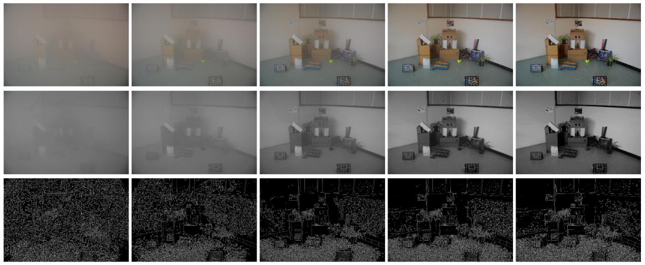
In order to evaluate the validity of Proposition 2, five images with different levels of fog density from [16] (first row) and their dark channel maps (second row) were studied and are presented in Figure 1. From this evaluation, we found that the brighter the dark channel image, the thicker the fog, i.e., the gray value tended toward 1 (0 is dark and 1 is white).
Usually, foggy images are blurrier and have low contrast, which means that edge information is also closely related to the fog density. This observation has been validated using a large set of images. As shown in the third row of Figure 1, the thicker the fog, the more pseudo-edge details. Due to the effects of the fog, the edges are pseudo-edges.
Our approach was based on the dark channel maps and pseudo-edge details of the images and the fog density index of the image was first defined as:
This is a logistic function, which is also called the sigmoid function, and its domain is the real number set and range of the open interval (0, 1). The use of Equation (2) meant that the relative fog density was defined based on the average value of the product of dark channels that were related and the proportion of the edge information. In this equation, and are the scaling parameters and is the translation parameter that was used in the standardization process. The three parameters were positive numbers and could be obtained by training the standard database.
Moreover, in Formula (2), , the pseudo-edge details of the image are the ratios of edge pixel points to image points and the edge image was obtained using the Canny operator [18]. The average brightness of the dark channel maps, except for the sky and white regions, in the images was represented by :
where m and n are the number of rows and columns in the image, is the number of non-sky pixels and is the segmentation parameter of the pixels in the sky and white image blocks, generally . was standardized as:
where is the standardized and and are two thresholds with experimental values of and , which were introduced to distinguish the sky and white regions, the foggy regions and the fog-free areas.
2.2. Fog Density Levels
According to application requirement, the fog density level of an image could be classified into four levels: fog-free, shallow fog, moderate fog and dense fog, which were represented by 0, 1, 2 and 3, respectively. That is, was a piecewise constant function:
Different from the manual methods [4], this paper estimated the density level of an image automatically, according to the fog density index :
The parameters and in Formula (6) were estimated using an analysis of a set of foggy images with fog level labels from several accessible databases, for example, the Cityscapes Dataset [19,20].
Our method for the estimation of parameters was based on the normal distribution hypothesis of the density value of each category obeying a normal distribution , . In general, . The probability density functions were denoted as . Our algorithm consisted of two main steps.
The first step was to estimate the values of the parameters using the ith class of images ( in Formula (5) and in Formula (2)).
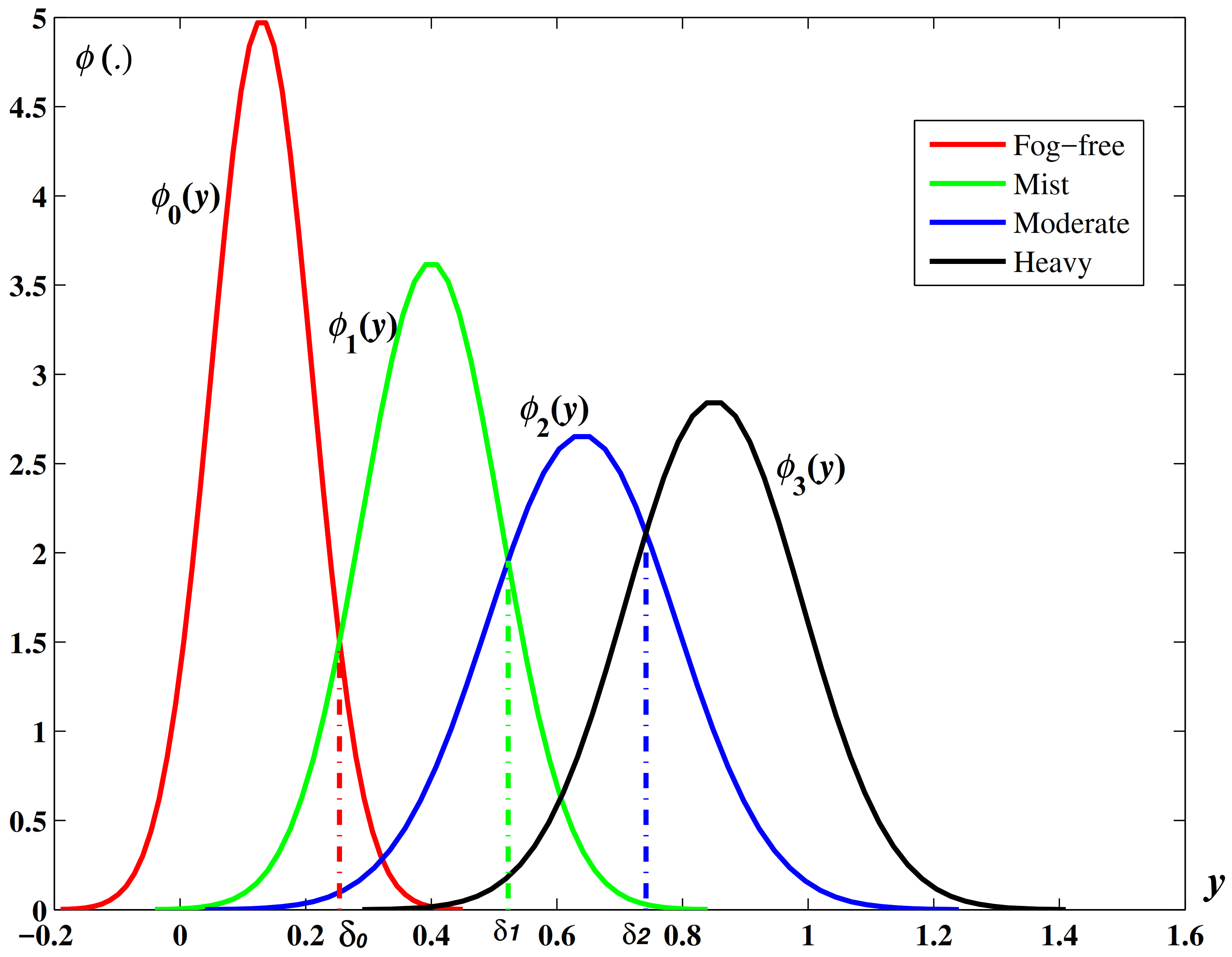
The second step was to calculate the parameters and by finding the intersection points between the adjacent probability density functions . These intersection points were successively marked as and , from small to big, as shown in Figure 2.
One of the advantages of the proposed method was that the probability of correct classification could be estimated theoretically. Here, we take the case of fog-free as an example:
Similarly, the probability of misclassification could be estimated as:
Theoretically, the probabilities of the correct classification or misclassification of all cases could also be calculated using similar formulae. The results formed a matrix, which was named as a confusion matrix (described in the next section).
By substituting the estimated values of and into Formula (6), the fog density level () of an image I could be determined according to its fog density value .
3. Results
In order to evaluate the proposed method, the experimental results are presented in this section. The experiments were conducted mainly for the estimation of fog density values and fog density levels in images, as well as changes of fog density in videos.
3.1. Fog Density Estimation
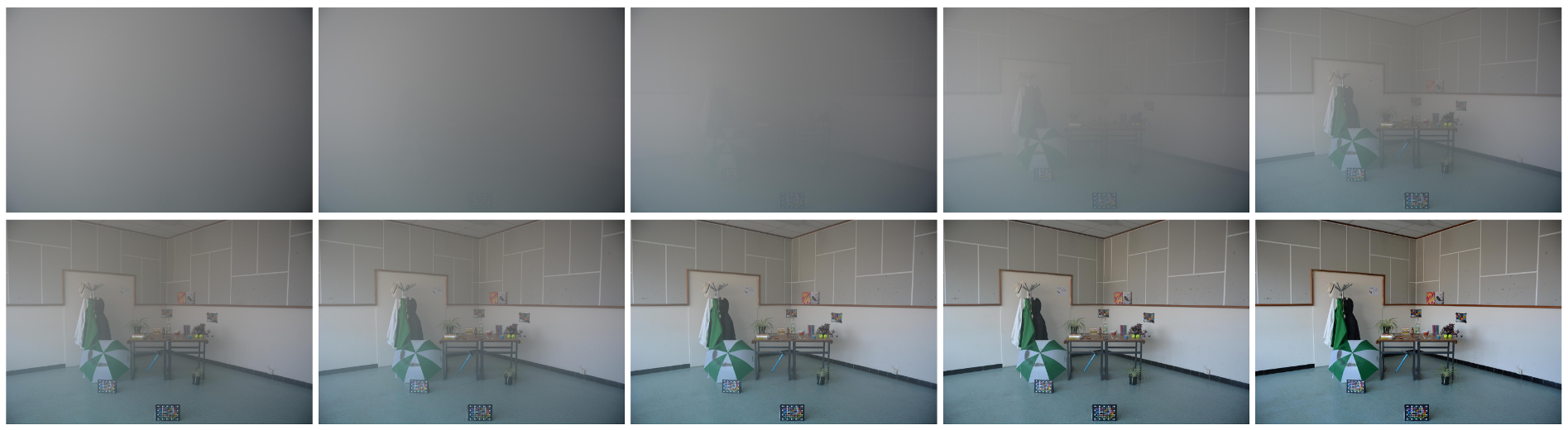
To verify the effectiveness of the fog density index , the of images from the Color Hazy Image Database (CHIC) [16] was calculated and compared to the results from SFDE [10], FADE [7] and the ground truth. Figure 3 shows 10 images from Scene1 in CHIC and these images are all labeled with a density from 1 (heavy foggy) to 10 (clear). Note that the CHIC database is characterized by the presence of the ground truth reference images.
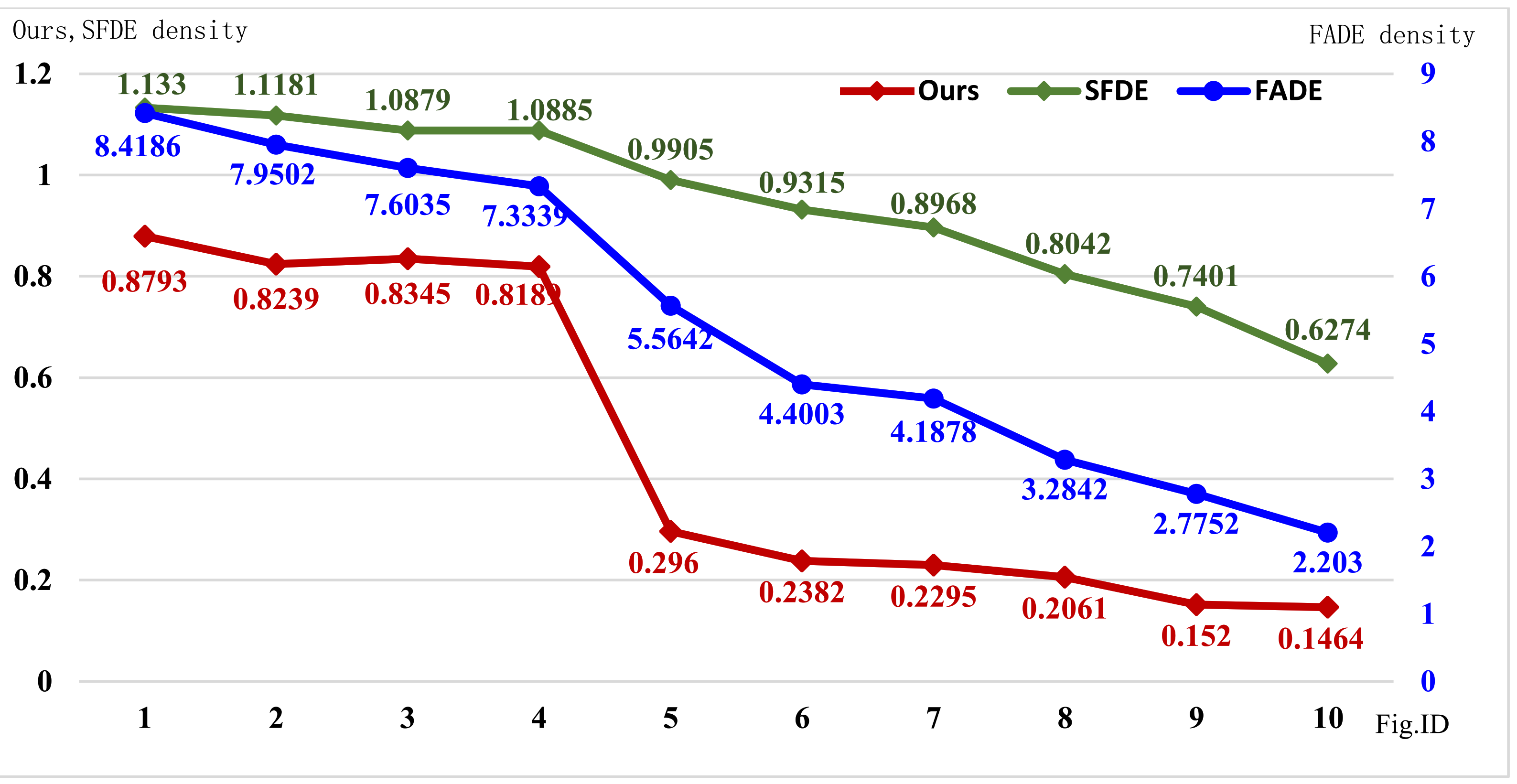
Figure 4 shows the fog density values that were evaluated using SFDE [10], FADE [7] and our method. By comparing these three curves, we found the following characteristics:
- (1)
- The three curves were all monotonically decreasing, which was highly consistent with the changes in the real fog density values of the images in the dataset (ground truth information);
- (2)
- The fog density values that were estimated using our method were limited to the interval 0 to 1, in which 0 meant clear and 1 represented heavy fog, while FADE did not have a limited interval and the density values that were calculated using SFDE tended to be greater than 0.5. Obviously, our fog density values had a more intuitive meaning;
- (3)
- Our curve was in sharp decline from the fourth image to the fifth image, which illustrated that the fog density in the first four images was significantly different from that in the last six images. This correlated with the real situation.
3.2. Fog Density Levels
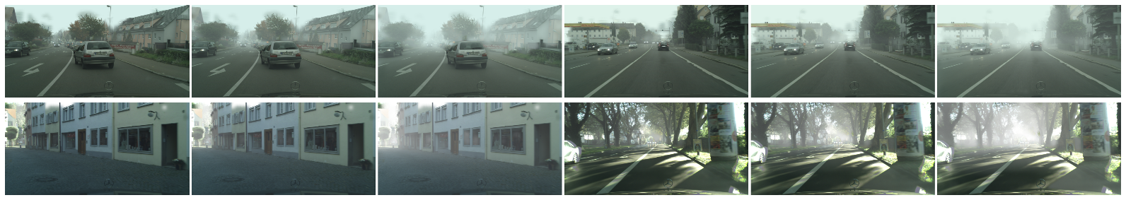
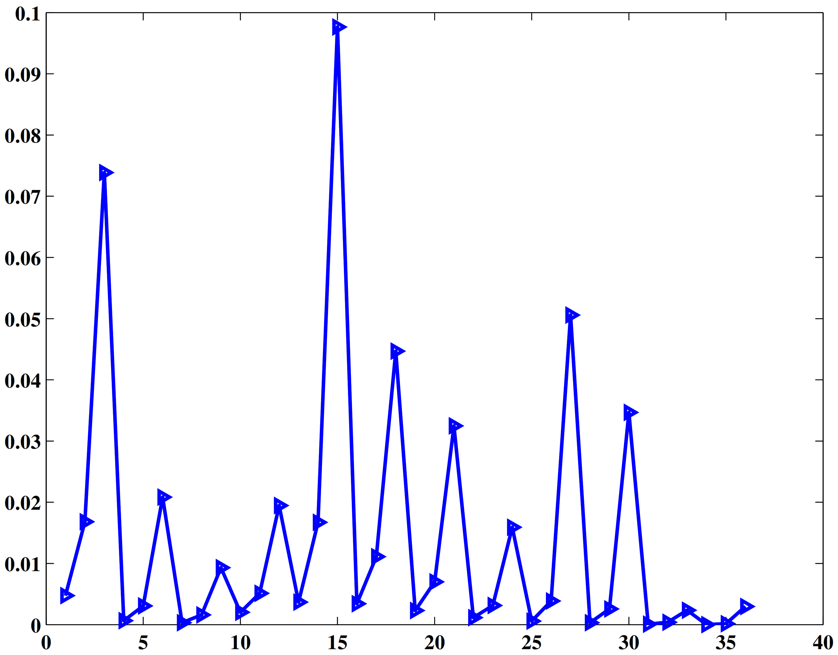
The other experimental dataset that we employed was “lindau”, which is a subset of the Cityscapes dataset [19,20]. The “lindau” dataset consists of 177 images, of which 59 images are covered with shallow fog, 59 are covered with moderate fog and 59 are covered with heavy fog. Figure 5 presents 12 images from four different scenes in the dataset. By applying Formula (2) to 36 of the images, which consisted of these 12 images covered with three different density levels of fog, the fog density values were calculated and are displayed in Figure 6. Figure 5 and Figure 6 show that the fog density in most of these images was very low. According to general standards, all of these images would be classified into the shallow fog category, both visually and numerically. However, this dataset divided the values into three different categories (shallow fog, moderate fog and heavy fog) based on a refined standard, which meant that in some application scenarios, it was necessary to distinguish the fog density levels within a small range of variation. Our method could realize this fine classification through parameter learning when the labeled training dataset was feasible.
In order to identify the density level according to the practice application, it was necessary to first calculate the value of parameter in Formula (2) and in Formula (6) using the training data. Since only three density levels (shallow, moderate and heavy) were considered, we did not need to estimate the parameter .
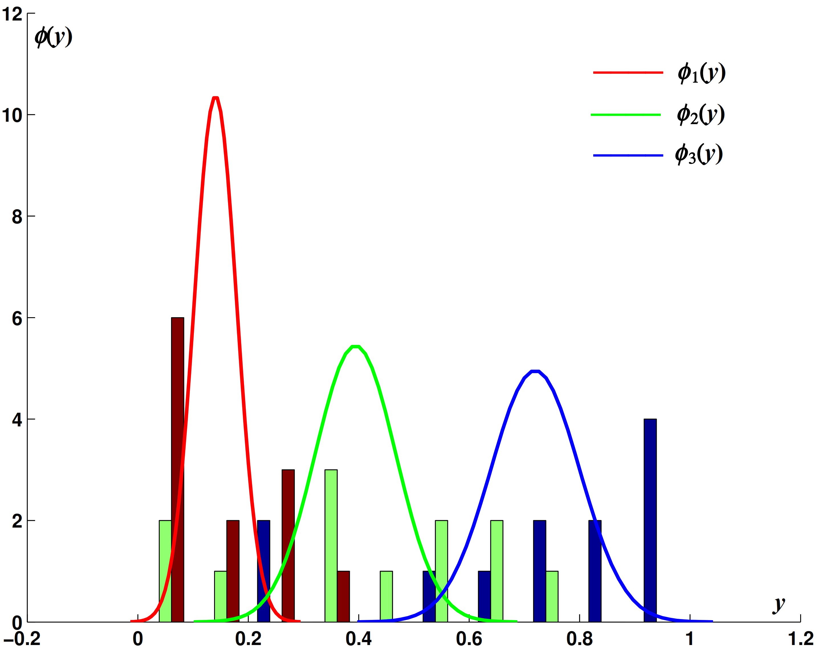
We chose the first 36 images (12 images with three fog densities) as the training data. Six of them are shown in the first row of Figure 5. After training, the parameters , and were evaluated as , and . The normal distribution fitting curves are shown in Figure 7. The confusion matrix of the training results is listed in the three left-hand columns of Table 1. The accuracy of the fog density level estimation was 0.9812.
The last 141 images (47 images with three fog density levels) in the “lindau” database were chosen as our test data. The confusion matrix of the test dataset is listed in the three right-hand columns of Table 1. The accuracy of the fog density level estimation was 0.6241.
3.3. Fog Density Levels in Videos
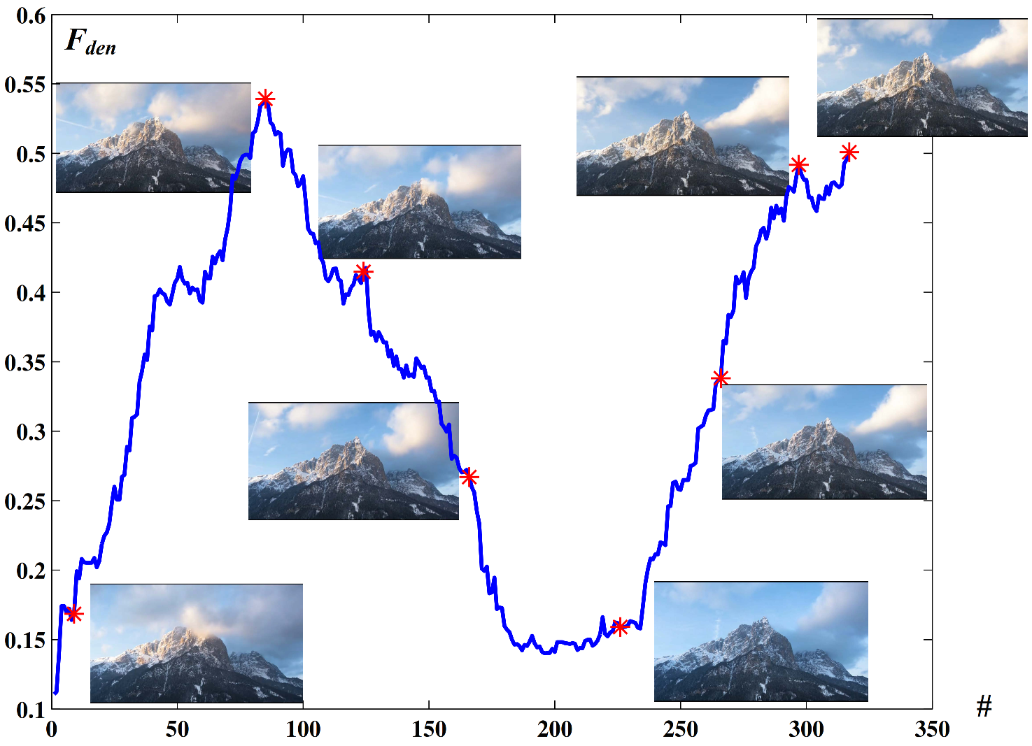
The fog density level of the scenes that were evaluated using a single image could predict changes in fog density during a video. We downloaded a video of foggy mountains (thanks to the open permission of the uploader) from the Bilibili website (https://www.bilibili.com/video/BV1Rb411y7qR?p=9 accessed on 17 May 2021). The first 12 s of the video, which is composed of 317 frames, was used as the experimental data. The fog density values of the frames were drawn as a discrete curve (for convenience, we called it the curve), which is shown in Figure 8, where the symbol “#” denotes the frame sequence number.
To evaluate the image defogging algorithms, various objective evaluation indexes have been adopted, such as the classical indexes “SSIM” and “PSNR” [21] and the recently proposed indexes “visible edge ratio” and “average gradient ratio” [22]. However, to evaluate the performance of video defogging algorithms, additional indexes are needed to evaluate the temporal and spatial coherence of the defogged results. Since could be used not only to measure the degree of image pollution and the image defogging effect but also changes in the fog density in a video, it was suitable for the evaluation of the video’s temporal and spatial coherence.
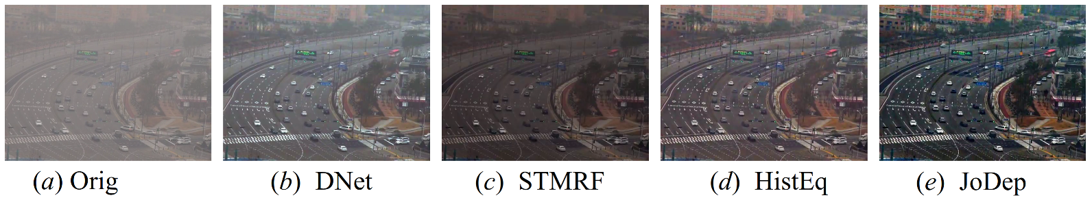
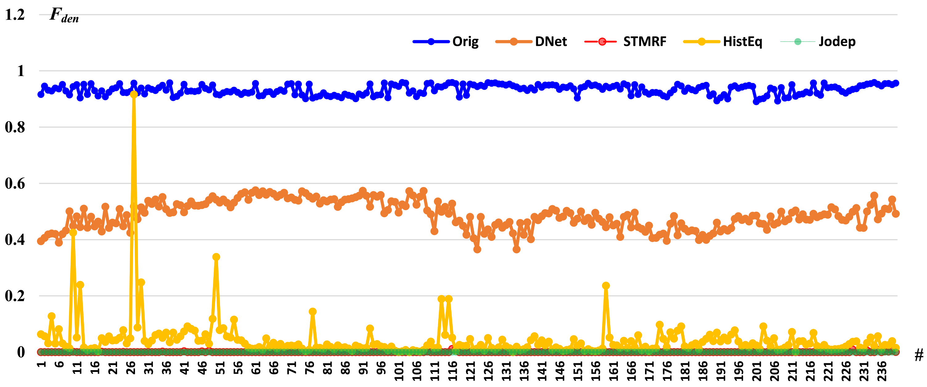
According to Equation (2), the fog density of each frame of the defogged video formed a sequence. We found that the changes in the sequence were closely related to the smoothness of the video, especially the defogged video. In general, the flatter the curve, the smoother the motion in the video. Conversely, violent fluctuations in the curve meant that the flicker of the dehazed video increased. To validate our observations, experiments were conducted on the foggy video “Cross” [23], which consists of 240 frames. Four existing video dehazing algorithms were evaluating using the curves. These four algorithms were: dehazing based on a neural network (DNet) [24], advanced histogram equalization (HistEq) [23], jointly estimating scene depth (JoDep) [25] and spatial–temporal MRF (STMRF) [26]. The experimental results are shown in Figure 9 and Figure 10. Figure 9 exhibits the defogged images of one frame that were produced by the four algorithms.
The curves of the original foggy video and the defogged videos that were produced by the four algorithms are displayed in Figure 10. It can be seen that the original video was taken under heavy fog weather conditions, the result of the DNet algorithm retained the most fog, the curve of HistEq algorithm shows the most and biggest fluctuations (which meant that there were the most flickers in that video) and the curves of the STMRF and JoDep algorithms were relatively smooth and almost coincided with the straight line Fden = 0 (which meant that the defogged videos had less flickers and the least amount of residual fog).
4. Conclusions
The aim of our method was to estimate the relative fog density by simply using an improved logistic function, which was related to the dark channel maps and pseudo-edge details of the images. The fog density values, which are directly proportional to the visibility, were standardized into the interval 0 to 1, which was conducive for the comparison of different images. For the practical application, we constructed an index of fog density levels using the estimated relative fog density values. The parameters that were involved in the level classification were estimated using a trained set of foggy images with fog level labels from several accessible databases. Due to this, the number of levels could be increased or decreased flexibly, according to the application requirements.
From the experimental results using open image datasets, several conclusions could be drawn:
- (1)
- In the experiment using the Color Hazy Image Database (CHIC), our index was consistent with the labeled fog density values in terms of rank order;
- (2)
- In the experiment using the Cityscapes database, our index was consistent with the labeled fog density values. The accuracy reached as high as 0.9812.
It should be noted that our method had its limitations. It did not uncover the quantitative relationship between visibility and fog density, which will become our research topic in the future. One approach that is also worth exploring is as follows: take photos and calculate the fog density levels using an image-based fog density estimation method (such as the proposed method) while measuring fog density via various meteorological sensors [2,27,28], then establish the quantitative relationship between the measured and estimated fog density values and improve the accuracy using multi-scene model correction. There is no doubt that the discovery of this relationship will promote the application of our method in image and video processing.
Author Contributions
Conceptualization, X.W. and H.L.; methodology, H.L.; software, H.G.; validation, H.G. and H.L.; formal analysis, X.W.; investigation, H.G.; resources, X.W.; data curation, H.G. and H.L.; writing—original draft preparation, H.G. and H.L.; writing—review and editing, X.W.; visualization, H.L.; supervision, X.W.; project administration, X.W.; funding acquisition, X.W. All authors have read and agreed to the published version of the manuscript.
Funding
This research was funded by the NSFC, grant number 61571046.
Institutional Review Board Statement
Not applicable.
Informed Consent Statement
Not applicable.
Data Availability Statement
Data used in this article are available from the authors upon request.
Acknowledgments
We would like to sincerely thank the authors of the FADE and SFDE algorithms for sharing their code. The constructive comments from anonymous reviewers were also greatly appreciated.
Conflicts of Interest
The authors declare no conflict of interest. The funders had no role in the design of the study, the collection, analyses or interpretation of data, the writing of the manuscript or the decision to publish the results.
References
- Jiang, Y.; Sun, C.; Zhao, Y.; Yang, L. Fog Density Estimation and Image Defogging Based on Surrogate Modeling for Optical Depth. IEEE Trans. Image Process. 2017, 26, 3397–3409. [Google Scholar] [CrossRef] [PubMed]
- Gultepe, I.; Milbrandt, J.; Belair, S. Visibility parameterization from microphysical observations for warm fog conditions and its application to the Canadian MC2 model. In Proceedings of the AMS Annual Meeting, San Antonio, TX, USA, 12–15 January 2006. [Google Scholar]
- Hareendran, T.K. Fog Detection: The Optical Route. Electronics for You, 23 January 2016. [Google Scholar]
- Zhao, S.; Zhang, L.; Huang, S.; Shen, Y.; Zhao, S. Dehazing Evaluation: Real-World Benchmark Datasets, Criteria, and Baselines. IEEE Trans. Image Process. 2020, 29, 6947–6962. [Google Scholar] [CrossRef]
- Lee, Z.; Shang, S. Visibility: How Applicable is the Century-Old Koschmieder Model? J. Atmos. Sci. 2016, 73, 4573–4581. [Google Scholar] [CrossRef]
- Caraffa, L.; Tarel, J.P. Daytime fog detection and density estimation with entropy minimization. ISPRS Ann. Photogramm. Remote. Sens. Spat. Inf. Sci. 2014, II-3, 25–31. [Google Scholar] [CrossRef] [Green Version]
- Choi, L.K.; You, J.; Bovik, A.C. Referenceless Prediction of Perceptual Fog Density and Perceptual Image Defogging. IEEE Trans. Image Process. 2015, 24, 3888–3901. [Google Scholar] [CrossRef] [PubMed]
- Yeh, C.H.; Kang, L.W.; Lee, M.S.; Lin, C.Y. Haze effect removal from image via haze density estimation in optical model. Opt. Express 2013, 21, 27127–27141. [Google Scholar] [CrossRef] [PubMed]
- Mori, K.; Takahashi, T.; Ide, I.; Murase, H.; Tamatsu, Y. Fog density recognition by in-vehicle camera and millimeter wave radar. Int. J. Innov. Comput. Inf. Control IJICIC 2007, 3, 1173–1182. [Google Scholar]
- Ling, Z.; Gong, J.; Fan, G.; Lu, X. Optimal Transmission Estimation via Fog Density Perception for Efficient Single Image Defogging. IEEE Trans. Multimed. 2018, 20, 1699–1711. [Google Scholar] [CrossRef]
- Liu, T.; Li, Z.; Mei, R.; Lai, C.; Wang, H.; Hu, S. The Visibility Measurement Based on Convolutional Neural Network. In Proceedings of the 2019 International Conference on Meteorology Observations (ICMO), Chengdu, China, 28–31 December 2019; pp. 1–3. [Google Scholar] [CrossRef]
- Xiyu, M.; Qi, X.; Qiang, Z.; Junch, R.; Hongbin, W.; Linyi, Z. An Improved Diracnet Convolutional Neural Network for Haze Visibility Detection. In Proceedings of the 2021 IEEE 31st International Workshop on Machine Learning for Signal Processing (MLSP), Gold Coast, Australia, 25–28 October 2021; pp. 1–5. [Google Scholar] [CrossRef]
- Tang, P.; Shaojing, S.; Tingting Zhao, T.; Li, Y. Visibility estimation of foggy weather based on continuous video information. Remote. Sens. Lett. 2021, 12, 1061–1072. [Google Scholar] [CrossRef]
- Li, R.; Kintak, U. Haze Density Estimation and Dark Channel Prior Based Image Defogging. In Proceedings of the 2018 International Conference on Wavelet Analysis and Pattern Recognition (ICWAPR), Chengdu, China, 15–18 July 2018; pp. 29–35. [Google Scholar] [CrossRef]
- Mei, W.; Li, X. Single Image Dehazing Using Dark Channel Fusion and Haze Density Weight. In Proceedings of the 2019 IEEE 9th International Conference on Electronics Information and Emergency Communication (ICEIEC), Beijing, China, 12–14 July 2019; pp. 579–585. [Google Scholar] [CrossRef]
- Khoury, J.E.; Thomas, J.B.; Mansouri, A. A Database with Reference for Image Dehazing Evaluation. J. Imaging Sci. Technol. 2018, 62, 010503.1–010503.13. [Google Scholar] [CrossRef]
- He, K.; Sun, J.; Tang, X. Single Image Haze Removal Using Dark Channel Prior. Pattern Anal. Mach. Intell. IEEE Trans. 2011, 33, 2341–2353. [Google Scholar]
- Canny, J. A computational approach for edge detection. IEEE Trans. Pattern Anal. Mach. Intell. 1986, 8, 679–698. [Google Scholar] [CrossRef] [PubMed]
- Cordts, M.; Omran, M.; Ramos, S.; Rehfeld, T.; Enzweiler, M.; Benenson, R.; Franke, U.; Roth, S.; Schiele, B. The Cityscapes Dataset for Semantic Urban Scene Understanding. In Proceedings of the IEEE Conference on Computer Vision and Pattern Recognition (CVPR), Las Vegas, NV, USA, 27–30 June 2016. [Google Scholar]
- Sakaridis, C.; Dai, D.; Van Gool, L. Semantic Foggy Scene Understanding with Synthetic Data. Int. J. Comput. Vis. 2018, 126, 973–992. [Google Scholar] [CrossRef] [Green Version]
- Ren, W.; Zhang, J.; Xu, X.; Ma, L.; Cao, X.; Meng, G.; Liu, W. Deep Video Dehazing with Semantic Segmentation. IEEE Trans. Image Process. 2019, 28, 1895–1908. [Google Scholar] [CrossRef] [PubMed]
- Peng, S.J.; Zhang, H.; Liu, X.; Fan, W.; Zhong, B.; Du, J.X. Real-time video dehazing via incremental transmission learning and spatial-temporally coherent regularization. Neurocomputing 2021, 458, 602–614. [Google Scholar] [CrossRef]
- Kim, J.H.; Jang, W.D.; Sim, J.Y.; Kim, C.S. Optimized contrast enhancement for real-time image and video dehazing. J. Vis. Commun. Image Represent. 2013, 24, 410–425. [Google Scholar] [CrossRef]
- Cai, B.; Xu, X.; Jia, K.; Qing, C.; Tao, D. DehazeNet: An End-to-End System for Single Image Haze Removal. IEEE Trans. Image Process. 2016, 25, 5187–5198. [Google Scholar] [CrossRef] [PubMed] [Green Version]
- Li, Z.; Tan, P.; Tan, R.T.; Zou, D.; Zhou, S.Z.; Cheong, L.F. Simultaneous video defogging and stereo reconstruction. In Proceedings of the 2015 IEEE Conference on Computer Vision and Pattern Recognition (CVPR), Boston, MA, USA, 7–12 June 2015; pp. 4988–4997. [Google Scholar] [CrossRef]
- Cai, B.; Xu, X.; Tao, D. Real-Time Video Dehazing Based on Spatio-Temporal MRF. In Proceedings of the Advances in Multimedia Information Processing—PCM 2016, Xi’an, China, 15–16 September 2016; Springer International Publishing: Berlin/Heidelberg, Germany, 2016; pp. 315–325, $10.1007/978-3-319-48896-7\_31$. [Google Scholar]
- Gultepe, I.; Milbrandt, J.A.; Zhou, B. Marine Fog: A Review on Microphysics and Visibility Prediction. In Marine Fog: Challenges and Advancements in Observations, Modeling, and Forecasting; Koračin, D., Dorman, C.E., Eds.; Springer International Publishing: Cham, Switzerland, 2017; pp. 345–394. [Google Scholar] [CrossRef]
- Gultepe, I.; Agelin-Chaab, M.; Komar, J.; Elfstrom, G.; Boudala, F.; Zhou, B. A Meteorological Supersite for Aviation and Cold Weather Applications. Pure Appl. Geophys. Vol. 2019, 176, 1977–2015. [Google Scholar] [CrossRef]
Figure 1.
Fog density and pseudo-edge details. The first row shows five images with different fog density values (from left to right, the fog density changes from high to low) [16]. The corresponding dark channel images and pseudo-edge details are presented on the second and third rows, respectively.

Figure 2.
Estimation of parameters using the intersection points of the adjacent normal distribution curves.
Figure 2.
Estimation of parameters using the intersection points of the adjacent normal distribution curves.

Figure 3.
Images from Scene1 of CHIC. From left to right, the fog density levels of the images in the first row are 1 (the highest) to 5 and those in the second row are 6 to 10 (the clearest image).
Figure 3.
Images from Scene1 of CHIC. From left to right, the fog density levels of the images in the first row are 1 (the highest) to 5 and those in the second row are 6 to 10 (the clearest image).

Figure 4.
Comparison of the fog density values that were estimated using SFDE [10], FADE [7] and our method.

Figure 5.
Sample images (four images with three fog density levels) from the “lindau” database [20].
Figure 5.
Sample images (four images with three fog density levels) from the “lindau” database [20].

Figure 6.
Fog density of the 36 sample images (12 images with three fog density levels) from the “lindau” database [20] evaluated using our method with default parameters.
Figure 6.
Fog density of the 36 sample images (12 images with three fog density levels) from the “lindau” database [20] evaluated using our method with default parameters.

Figure 7.
Frequency statistical histogram and normal distribution fitting curves of fog density levels of the 36 training images. Different color means different fog density level.
Figure 7.
Frequency statistical histogram and normal distribution fitting curves of fog density levels of the 36 training images. Different color means different fog density level.

Figure 8.
The changes in fog density value during the video.

Figure 9.
A sample frame from the original video and the defogged images from the four different video defogging algorithms.
Figure 9.
A sample frame from the original video and the defogged images from the four different video defogging algorithms.

Figure 10.
curves of the original video and the four different video defogging algorithms.


Table 1.
The accuracy of fog density level estimation in the training stage and the test (marked with “*”) stage.
Table 1.
The accuracy of fog density level estimation in the training stage and the test (marked with “*”) stage.
| Level | ||||||
|---|---|---|---|---|---|---|
| Shallow | 0.9929 | 0.0071 | 0.0000 | 0.9149 | 0.0426 | 0.0426 |
| Moderate | 0.0149 | 0.9689 | 0.0162 | 0.4894 | 0.2553 | 0.2553 |
| Heavy | 0.0000 | 0.0181 | 0.9819 | 0.1489 | 0.1489 | 0.7021 |
Publisher’s Note: MDPI stays neutral with regard to jurisdictional claims in published maps and institutional affiliations. |
© 2022 by the authors. Licensee MDPI, Basel, Switzerland. This article is an open access article distributed under the terms and conditions of the Creative Commons Attribution (CC BY) license (https://creativecommons.org/licenses/by/4.0/).
Share and Cite
MDPI and ACS Style
Guo, H.; Wang, X.; Li, H. Density Estimation of Fog in Image Based on Dark Channel Prior. Atmosphere 2022, 13, 710. https://0-doi-org.brum.beds.ac.uk/10.3390/atmos13050710
AMA Style
Guo H, Wang X, Li H. Density Estimation of Fog in Image Based on Dark Channel Prior. Atmosphere. 2022; 13(5):710. https://0-doi-org.brum.beds.ac.uk/10.3390/atmos13050710
Chicago/Turabian StyleGuo, Hong, Xiaochun Wang, and Hongjun Li. 2022. "Density Estimation of Fog in Image Based on Dark Channel Prior" Atmosphere 13, no. 5: 710. https://0-doi-org.brum.beds.ac.uk/10.3390/atmos13050710
Note that from the first issue of 2016, this journal uses article numbers instead of page numbers. See further details here.