European Grid Dataset of Actual Evapotranspiration, Water Availability and Effective Precipitation

Abstract

The sustainability of a territory is closely related to its resources. Due to climate change, the most precious natural resource, water, has been negatively affected by climatic conditions in terms of quantity and quality. CLIMAT datasets of 1 km² spatial resolution were used and processed in the ArcGIS environment to generate maps of actual evapotranspiration, water availability, and effective precipitation for the periods of 1961–1990 (1990s), 2011–2040 (2020s), and 2041–2070 (2050s). The product is of paramount importance for the analysis of the actual situation in Europe indicating high water availability in the Alps Range, the Carpathians Mountains, Northern European countries, and the British Islands. On the other hand, low water availability has been evidenced in the Southern and Eastern European areas. For the future period (2050s), the monthly potential evapotranspiration is expected to increase by 30%. The climate models also show an increase in the actual evapotranspiration between past and future periods by 40%. The changes in water availability and effective precipitation between the past (1990s) and future (2050s) indicate decreases of 10%. The most affected areas by climate change are located within the Mediterranean areas, the Iberian Peninsula, and Eastern Europe.

1. Introduction

Surface water and groundwater are important resources at a global level. In most cases, the renewal of water resources is dependent upon the climate regime. Precipitation and temperature-related climate data are the main parameters that influence long-term water resources [1]. In recent decades, global climate change has led to major differences in temperature and precipitation records. These differences were found to have a direct negative influence on water resources and environmental elements at a global level [2,3]. Due to the lack of knowledge of environmental changes, the inadequate management of natural resources and inefficient strategies, the impact of climate change on water resources has been greater than was expected, contributing to limited resources and affecting conservation and sustainability [4,5,6]. In several areas of the globe, the negative impact of climate change on the glaciers and water systems is now evident. Moreover, the anthropic factor has frequent negative influence on the status of the environment both at a qualitative and quantitative level [7]. Industrial activities and agricultural practices contribute to the increase in the pressure placed on water resources and environmental elements [8,9,10].

In the European continent, the status of the water resources is determined by water availability and by the quality of surface water and groundwater. Water availability depends on the precipitation regime, which is strictly related to the mean air temperature, a key parameter for the evapotranspiration of hydrogeological basins together with the land cover pattern [11,12]. When comparing the historical climate data series, an increase in the mean annual temperature was observed. In addition, several climate models indicate that global warming has resulted in higher temperatures in the 21st century [13,14,15]. One of the most significant indicators is the rate of glacier melting [16,17]. The melting of ice and considerable retreating of glaciers observed in recent decades [18,19] influences the water resources in respective regions [20].

Hydrogeologists and environmental scientists have analyzed the climatic data from the actual measurements of instruments. They observed that global warming was higher in recent decades as compared to the past [21,22] with a major impact on water resources [23,24]. They deduced that the negative effect of climate change does not only impact runoff and groundwater recharge but also various components of the ecosystems [25,26]. In addition, a joint study of industrial activities and agricultural practices indicated that changes in the pattern of water resources were reflected in watersheds, surface water, land evapotranspiration, and groundwater levels. In the coastal areas, seawater intrusion due to the rise of the sea level has prompted the degradation of freshwater and a decrease in the quality of groundwater in the coastal aquifers [4,24].

Considering that it is an overall heterogeneous continent, the status of water resources in Europe varies from one region to another depending on each region’s climatic conditions and whether they are located in lowlands or high mountains. Thus, the southern areas of the continent are subjected to the Mediterranean climate with long, dry periods during the hydrological year. The eastern areas are influenced by the continental climate with low precipitation during summertime, while the western and northern parts of Europe are subjected to humid climates with higher rates of precipitation during the winter season. In this study, we aimed to analyze the temporal and spatial variation of water availability across Europe in three main periods, including the 1990s, 2020s, and 2050s. To deliver the required data grids of climate and water resources for the risk assessment, the terrain morphology, climate, and water availability datasets were analyzed both at a temporal and spatial scale, especially for the mid-21st century.

2. Study Area

The European continent is very complex and unique from several points of view. The extension of a latitudinal weight and the occurrence of a multitude of mountain units and large oceanic masses are major climate-influencing factors. Keeping these factors in mind, it should be mentioned that the orography of the European continent is diverse, with the majority of the land area consisting of plains and hills. The mountain chains include the Scandinavian Mountains in the North, the Alps Range and Apennine chains in the South, Pyrenees chain in the West, Carpathians Mountains in the central part, and Ural chain in the East. In addition, the Scottish Mountains dominate in the British Islands. Orography and the climate influences control the climate types and the precipitation regime. Thus, the availability of water is strongly dependent on the rainfall rate and is extremely variable along the European continent.

From the climate point of view, the northern part of Europe has a Baltic climate, while the western and central parts of Europe are subject to Atlantic Ocean influence, the southern part of Europe has a Mediterranean influence, and the eastern part of Europe is under the influence of a continental climate. Hence, the European continent has several temperate climates, mostly with four seasons per year. According to the Koppen–Geiger climate classification, a fully humid warm temperate climate with warm summers (Cfb class) is typical of the central part of the continent [27]. The western part of Europe is influenced by the Atlantic Ocean, with a warm temperate climate with a hot and dry summer (Csa) and a warm temperate climate with a dry and warm summer (Csb), while the eastern part of Europe has a fully humid cold climate (Dfa and Dfb). The southern part mainly has a fully humid warm temperate climate with a hot summer (Cfa), while the northern part is in a fully humid cold temperate climate with a cool summer (Dfc) [27].

3. Materials and Methods

3.1. Climate Data

The climate data used in this work include mean monthly values of temperature and precipitation over 1961–2070, derived using the following three datasets: 1961–1990 (1990s) as historical records and two future models for the 2011–2040 (2020s) and 2041–2070 (2050s) periods. These datasets were processed for the European continent by Andreas Hamann [28] using 1 km² spatial resolution. The Parameter Regression of Independent Slopes Model (PRISM) was used to obtain the precipitation models. For the temperature model, the ANUSplin interpolation method was applied and a moderate climate change projection with emissions of RCP 4.5 was applied. This scenario mimics the global prediction increase of +1.4 °C (±0.5)29. The outcome of precipitation and temperature are raster data of ENSEMBLE climate models, representing an average of 15 AOGCMs as considered by the CMIP5 multi-model dataset. The procedure applied by Andreas Hamann is in line with IPCC Assessment Report 5 (IPCC, 2013). ClimateEU v4.63 environment was used to perform the climate models. The software is available at the website http://tinyurl.com/ClimateEU, accessed on 1 February 2022.

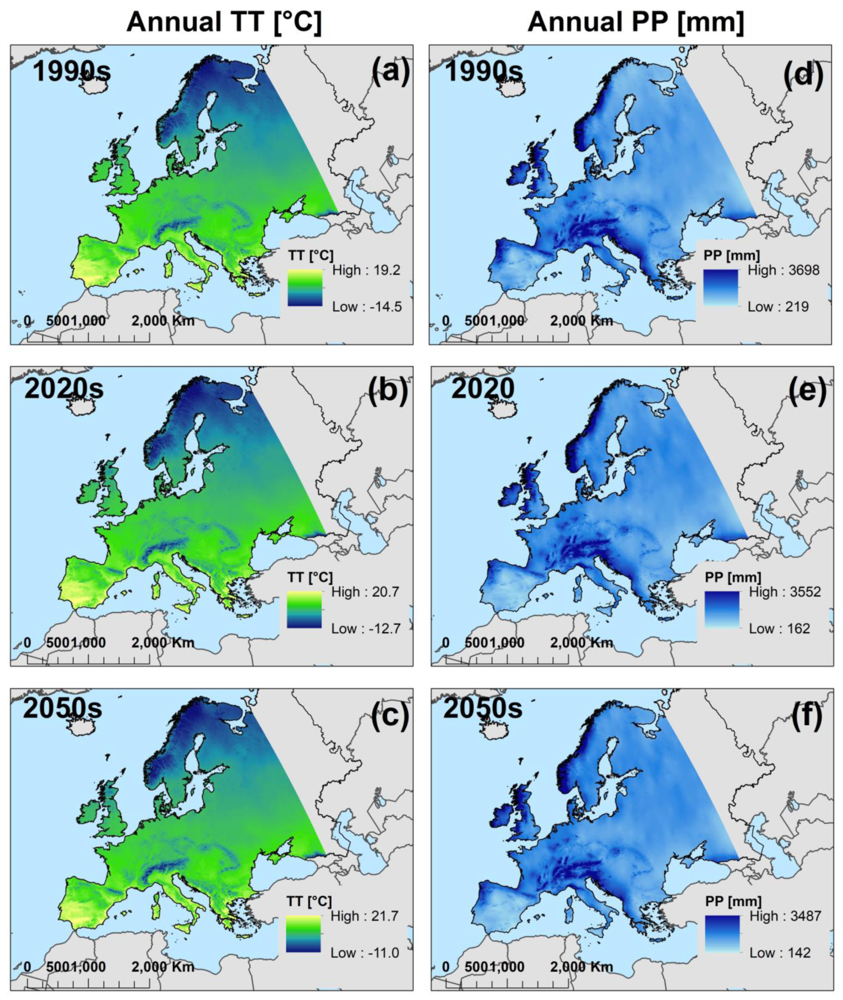
During the 1990s, the mean air temperature varied in Europe from −14.5 °C to 19.2 °C (Figure 1a). For the 2020s, the mean air temperature ranges between −12.7 °C and 20.7 °C (Figure 1b). In the period 2050s, the temperature models indicate values between −11 °C and 21.7 °C (Figure 1c). The higher values of temperature (above 15 °C) were depicted in West and South Europe, mainly in Spain and Italy. The lower values of temperature (<0 °C) were found in Northern Europe and in high-mountain areas such as the Alps, Pyrenes, and Carpathians.

During the 1990s, annual precipitation values ranged from 219 mm to 3698 mm (Figure 1d). For the future periods, the annual precipitation values will range between 162 mm and 3552 mm in the 2020s (Figure 1e) and 142 mm and 3487 mm in the 2050s (Figure 1f). The higher values of precipitation (above 3000 mm) were found in the South-central part of Europe, in the Alps and Dinaric Mountains, in the British Islands, and the Scandinavian Peninsula. The lower values of precipitation (below 400 mm) were identified in East Europe and the Iberian Peninsula.

Using temperature and precipitation climate models, the alfa parameter (α), the heat index (I), potential evapotranspiration (ET0), actual evapotranspiration (AET0) and water availability (WA) were calculated at the spatial scale of Europe.

3.2. Geological Data and Aquifers

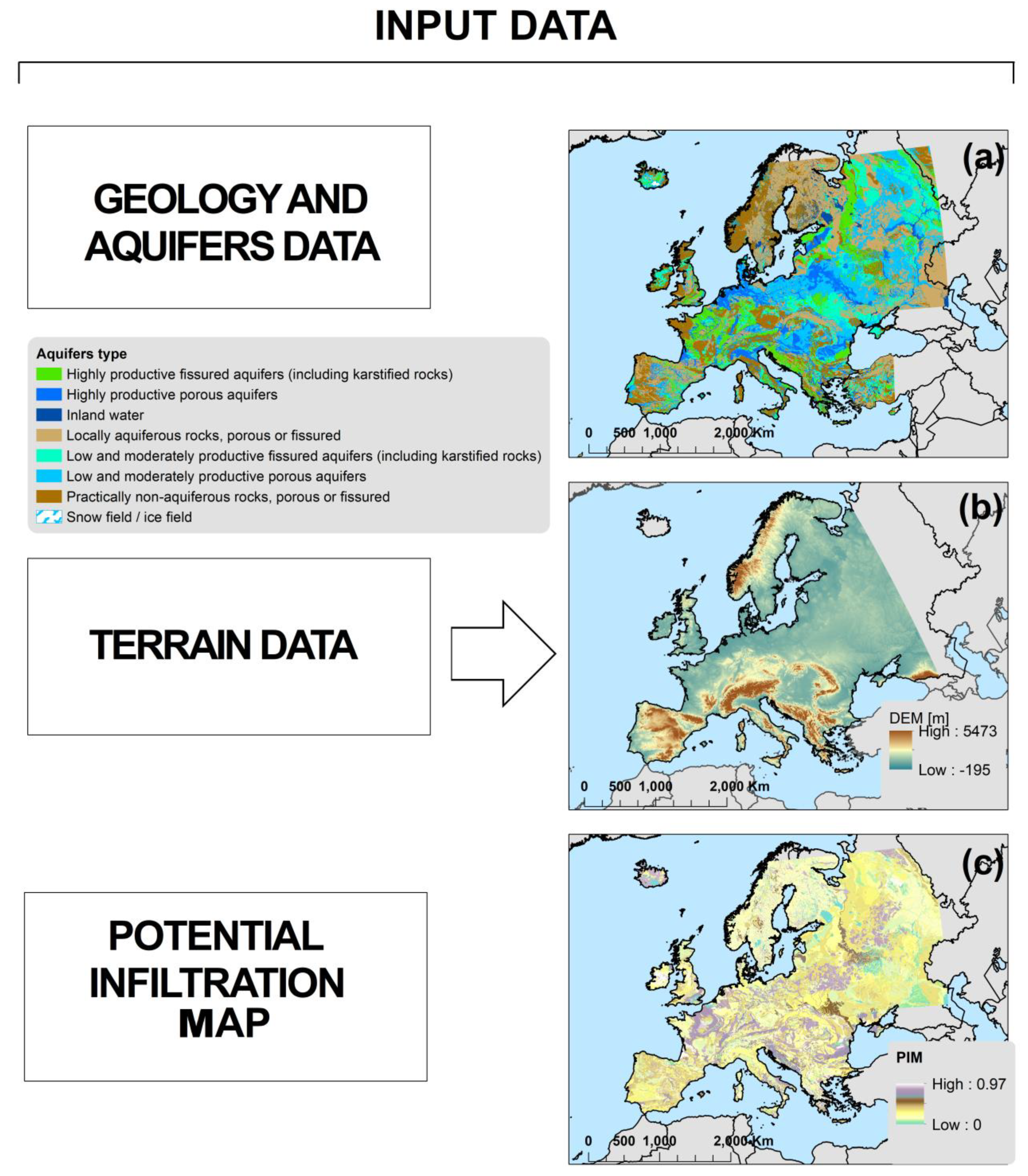
The International Hydrogeological Map of Europe, from 2013, at a 1:1,500,000 scale [29,30], was used in this study to differentiate the main geological formations and to identify the main types of aquifers in Europe. The European continent presents several geological formations of different ages including jointed and karstified rocks such as limestones, chalkstones, sandstones, conglomerates, volcanic and plutonic rocks, but also gneisses, marls, clays, shales, mica schists, quartzites in the mountains and hilly areas. The plains and lowlands are geologically composed of gravels, sands, silts, and clays. Considering the nature of the substrates, the following six types of productivity aquifers were defined in the International Hydrogeological Map of Europe: highly productive fissured aquifers, highly productive porous aquifers, low and moderately productive fissured aquifers, low and moderately productive porous aquifers, locally aquiferous rocks-porous or fissured, and practically non-aquiferous rocks-porous or fissured (Figure 2a). In this work, the geological and aquifers data are presented as vector data.

The lithology of the layers and the morphology of the terrains have a direct influence on the runoff, water availability (WA), control and infiltration rate into the soil. The infiltration water derives from WA and is defined as effective precipitation. The effective precipitation contributes to the recharging of aquifers and the soil water content [31].

3.3. Terrain Data

The terrain morphology controls the flow direction of surface waters. To estimate the potential infiltration of water, the Digital Elevation Model (DEM) of Europe, at a 1 km² spatial resolution was considered. From the DEM, the slope angle map was derived and used for the potential infiltration map calculation. According to the current DEM, the altitudes across Europe vary from −195 m to 5473 m asl (including the Caucasus Mountains) (Figure 2b).

The calculations and raster-data processing were performed in the ArcGIS environment.

3.4. Potential Infiltration Map

Based on the geological nature of the layers, DEM, and slope raster data maps, a potential infiltration map of Europe was created. The calculation considers higher infiltration values where the potential infiltration coefficient (PIC) is higher and the slope angle is lower. On the other hand, the infiltration values are lower where the PIC is lower and the slope angle is higher.

The method was previously applied in groundwater studies [9,32] and is important in the analysis of water resources and in the evaluation of environmental risks due to its complex correlation with hydrological processes. Thus, the potential infiltration map contains the permeability of the lithology through PIC and water flow direction through slope angle. These values have been determined in the laboratory by experts in hydrogeology and were tested in various studies [33,34] The infiltration process depends on permeability, the saturation of the soil, and pore-water pressure in the media [35,36]. The potential infiltration map (PIM) was calculated using the ratio between PIC and slope angle [33] (normalized values):

PIM = PIC/Slope angle

(1)

The PIC values for the aquifers are specific values chosen by experts in the CC-WARE European Project and DRINK Adria Project. Supplementary Material (Table S1) reports the PIC values used in this study.

3.5. Potential Evapotranspiration

We used the Thornthwaite method [34] to calculate the potential evapotranspiration (ET0). The method requires monthly temperature records. Even though it is a simple method (Equation (2)), it is still used in hydrology and climatology for various analyses, especially for the long-term period [2,26]. The other methods used in the ET0 calculation required more data, e.g., wind speed, solar radiation, humidity, and not all of these parameters are available for Europe from 1961 to 1990. In addition, the predictions of these parameters for the future will lead to more uncertainties. For this reason, the Thornthwaite formula was used in this study.

$$ET0=16{\left(\frac{10Ti}{I}\right)}^{\alpha }\hspace{1em}\hspace{1em}\hspace{1em}[\mathrm{mm}/\mathrm{month}]$$

(2)

where:

ET0—potential evapotranspiration;

T_i—monthly air temperature;

I—annual heat index (see Equation (3));

α—complex function of heat index (see Equation (4)).

$$I={{\displaystyle {\sum }_{i=1}^{12}\left(\frac{Ti}{5}\right)}}^{1.514}$$

(3)

$$\alpha =6.75\times {10}^{-7}{I}^3-7.71\times {10}^{-5}{I}^2+1.7912\times {10}^{-2}I+0.49239$$

(4)

3.6. Actual Evapotranspiration (AET0)

In this work, the actual evapotranspiration (AET0) was calculated based on annual ET0 and annual precipitation using the Budyko equation [37,38] (Equation (5)):

$$\frac{\mathrm{AET}0}{\mathrm{PP}}={\left[\left(\mathsf{\phi }\tan \frac{1}{\mathsf{\phi }}\right)\left(1-{\exp }^{-\mathsf{\phi }}\right)\right]}^{0.5}$$

(5)

where:

AET0—actual land cover evapotranspiration [mm]

PP—total annual precipitation [mm]

Φ—aridity index expressed as (Equation (6)):

$$\mathsf{\phi }=\frac{\mathrm{ET}0}{\mathrm{PP}}$$

(6)

The Budyko approach is a very useful method for the determination of AET0. It is widely applied in hydrological studies because it contributes not only to the water balance calculation but also it indicates if the heat energy is high enough to generate evaporation from precipitation [39]. The method also shows good performance [2,40] in climatology and agricultural studies. In this study, the AET0 contributes to the WA calculation and to the calculation of effective precipitation over Europe.

3.7. Water Availability (WA)

The water availability or runoff is the amount of water expressed as the difference between precipitation and AET0.

WA at the continental scale of Europe is of paramount importance for the evaluation of water resources in human life and its related activities, agriculture and industry. At the same time, the environmental issues are all closely related to water resources. In fact, they can benefit greatly from WA and in this case, some risks should be evaluated. Conversely, some zones could be positively affected by a higher amount of WA and the benefits and development in the respective areas could be considered.

3.8. Effective Precipitation

Effective precipitation is the amount of water that is able to infiltrate soil. Practically, effective precipitation is the amount of WA that is not retained as runoff water but most likely becomes groundwater. In geotechnical terms, effective precipitation and its related variables are very important parameters. Soil saturation plays a key role in effective precipitation and in related calculations for the slope stability, shear strength, and factor of safety. The climate regime, rock permeability, and terrain configuration determine the infiltration process and the amount of effective precipitation. Thus, all these factors have been considered in this study to determine the effective precipitation in Europe. A simple way to calculate the EP is to calculate the difference between precipitation and evapotranspiration [41]. After integrating the geological layer into the calculation, the most appropriate approach is achieved using the product between WA and PIM [42]. Assuming that this work was carried out at a continental scale and that it focused on the long-term period (averages of 30 years), we decided to calculate the effective precipitation as a product of water availability and a potential infiltration map, which is a simple ‘steady-state’ model (Equation (7)):

EP = WA × PIM

(7)

where:

EP—Effective precipitation [mm];

WA—Water availability [mm];

PIM—Potential infiltration map [dimensionless].

For the effective precipitation calculation, a normalization raster of PIM was used [43]. The procedure for the calculation of the effective precipitation takes into account the subsurface hydrologic properties, lithology, soil infiltration capacity, and slope as defined in previous specialty studies [41,44].

3.9. Data Normalization

For this study, the PIC, PIM, and slope angle maps were normalized, and the datasets were homogenized with values between 0 and 1. In order to obtain a comprehensive database with WA and effective precipitation, the maps were normalized and processed on a unique scale. The WA and effective precipitation datasets were then ready to use for spatial analyses for various applications, e.g., risk mapping of drought, flooding forecast, groundwater vulnerability, and factor of safety. The standard formula of normalization (Equation (8)) was used in this study:

X norm = (X − Xmin)/(Xmax − Xmin)

(8)

where:

X—the values in series;

Xnorm—the value after normalization;

Xmax—the maximum values in the series;

Xmin—the minim value in the series.

4. Results

4.1. Variation of Alfa Parameter (α), Heat Index (I), and Potential Evapotranspiration (ET0)

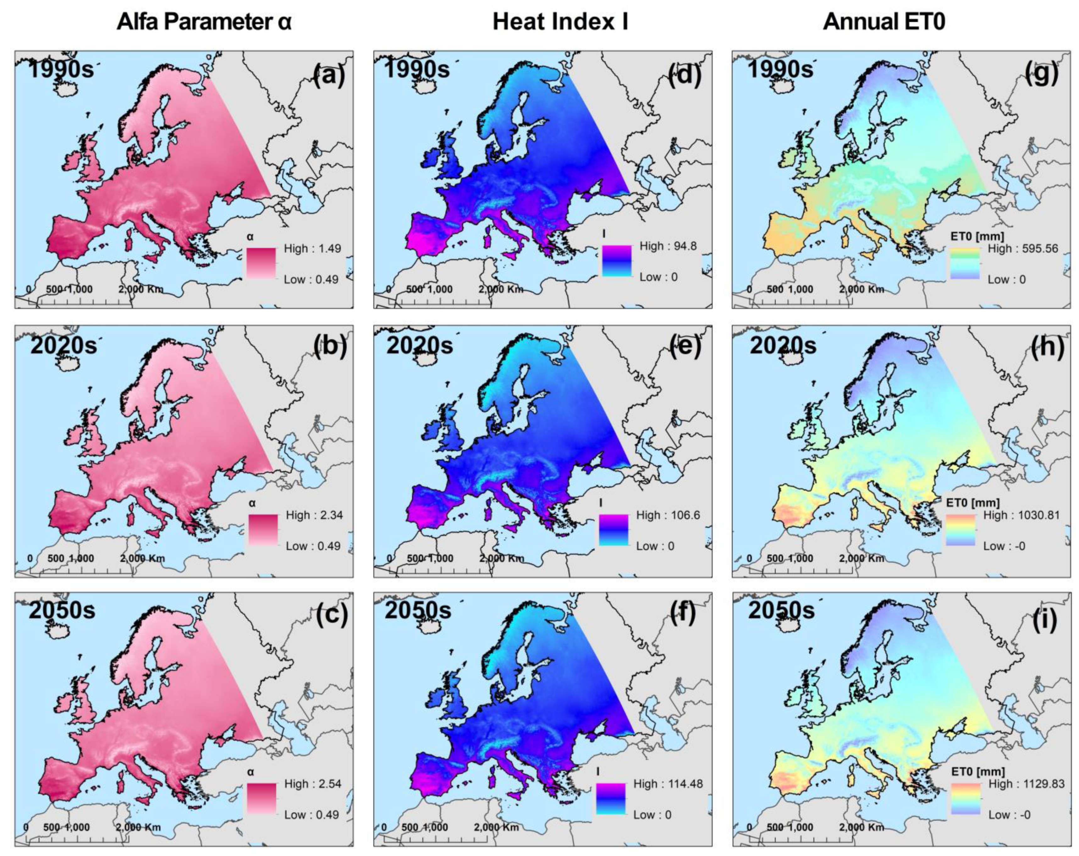
Two main constants derived from the temperature values that permit the calculation of the potential evapotranspiration calculation (ET0) are the alfa parameter (α) and heat index (I). At the spatial scale of Europe, α reaches values of up to 1.49 (in the 1990s), 2.34 (in the 2020s), and 2.54 (in the 2050s) in the Italian and Iberian Peninsulas, while the lower values were found in the mountain areas for all three periods. Figure 3a–c show the spatial distribution of α in Europe.

The heat index I in Europe varies from 0 to 94.8 in the 1990s, from 0 to 106.6 in the 2020s, and from 0 to 114.48 in the 2050s. The minimum values are found in the North of Europe and in the high mountains, where the temperature values are 0 °C and below. The higher values of I (>0.8) were identified in the West, South and South-East of Europe, where the temperature values are close to or above 20 °C. Figure 3d–f show the spatial distribution of I in Europe.

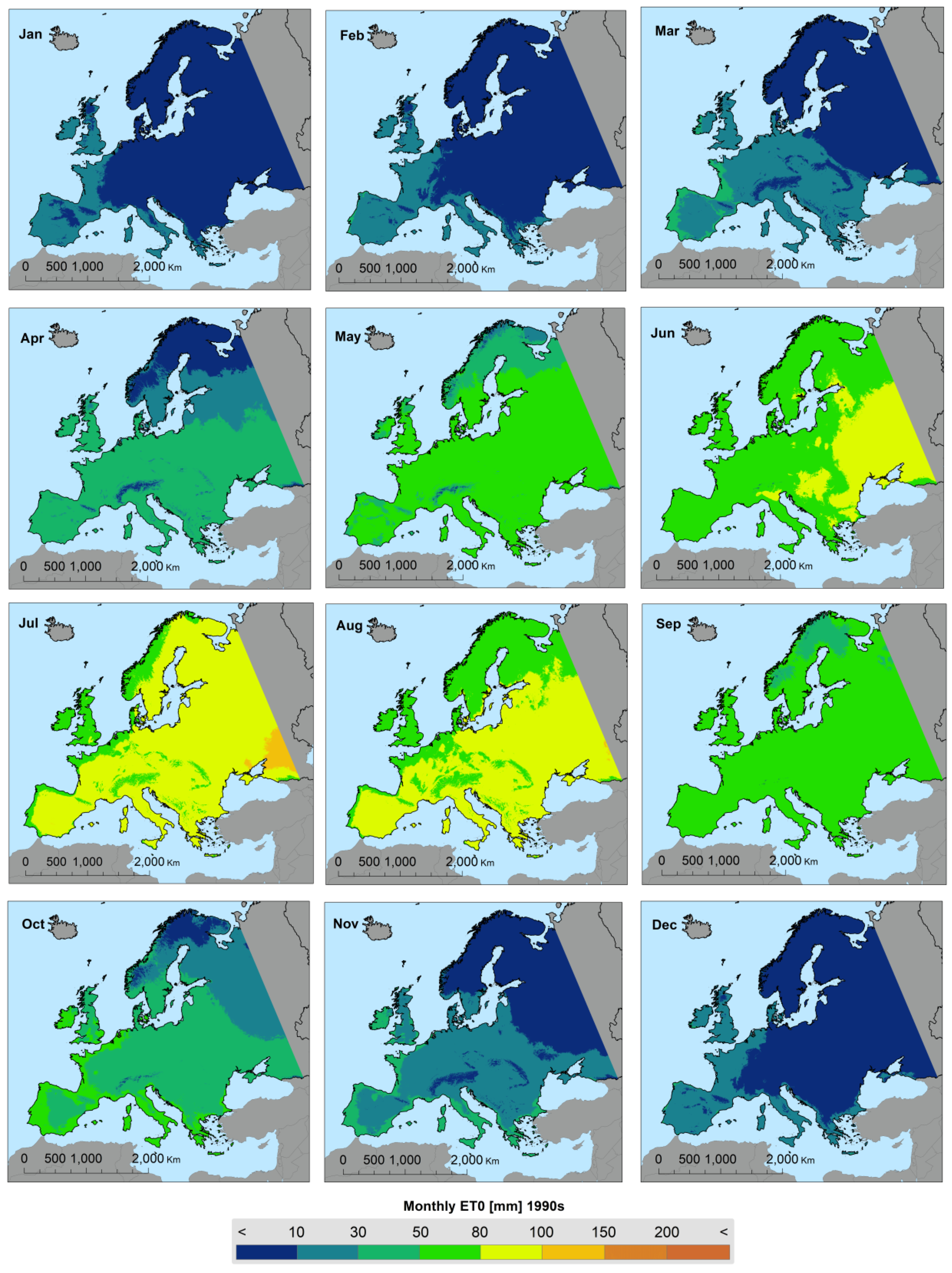
The monthly potential evapotranspiration (ET0) in Europe during 1990s–2050s was calculated using the Thornthwaite approach [34]. Despite being an older method for the determination of potential evapotranspiration, this approach is still very useful for hydrological studies and for long-term period [32,35,36,37]. In Europe, the monthly ET0 varied from 0 mm to 250 mm during the 1990s, with the higher values in July and August (over 200 mm) and lower values in the months of January, February, March, November and December. Figure 4 shows the monthly ET0 over the European continent during the 1990s.

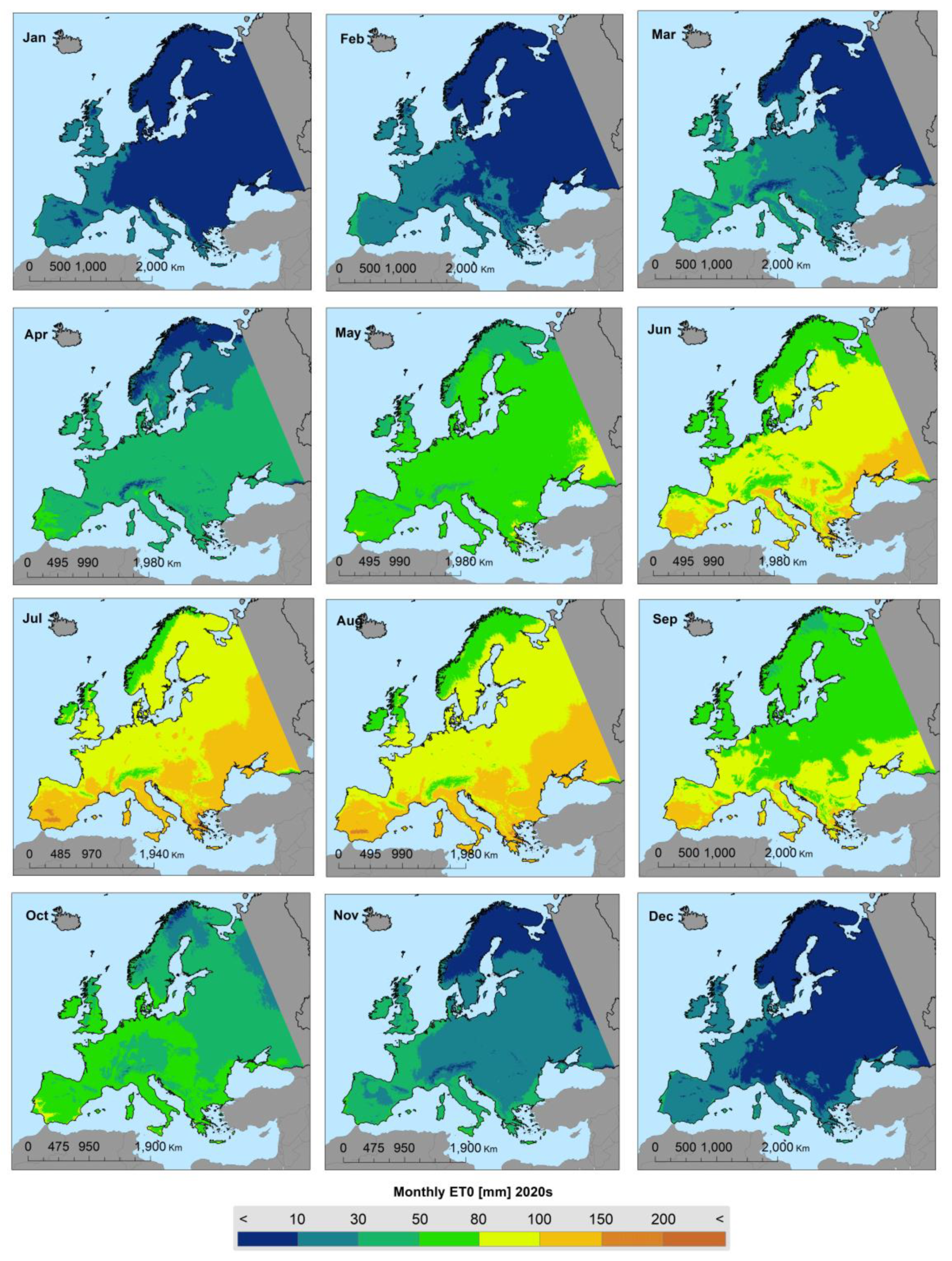
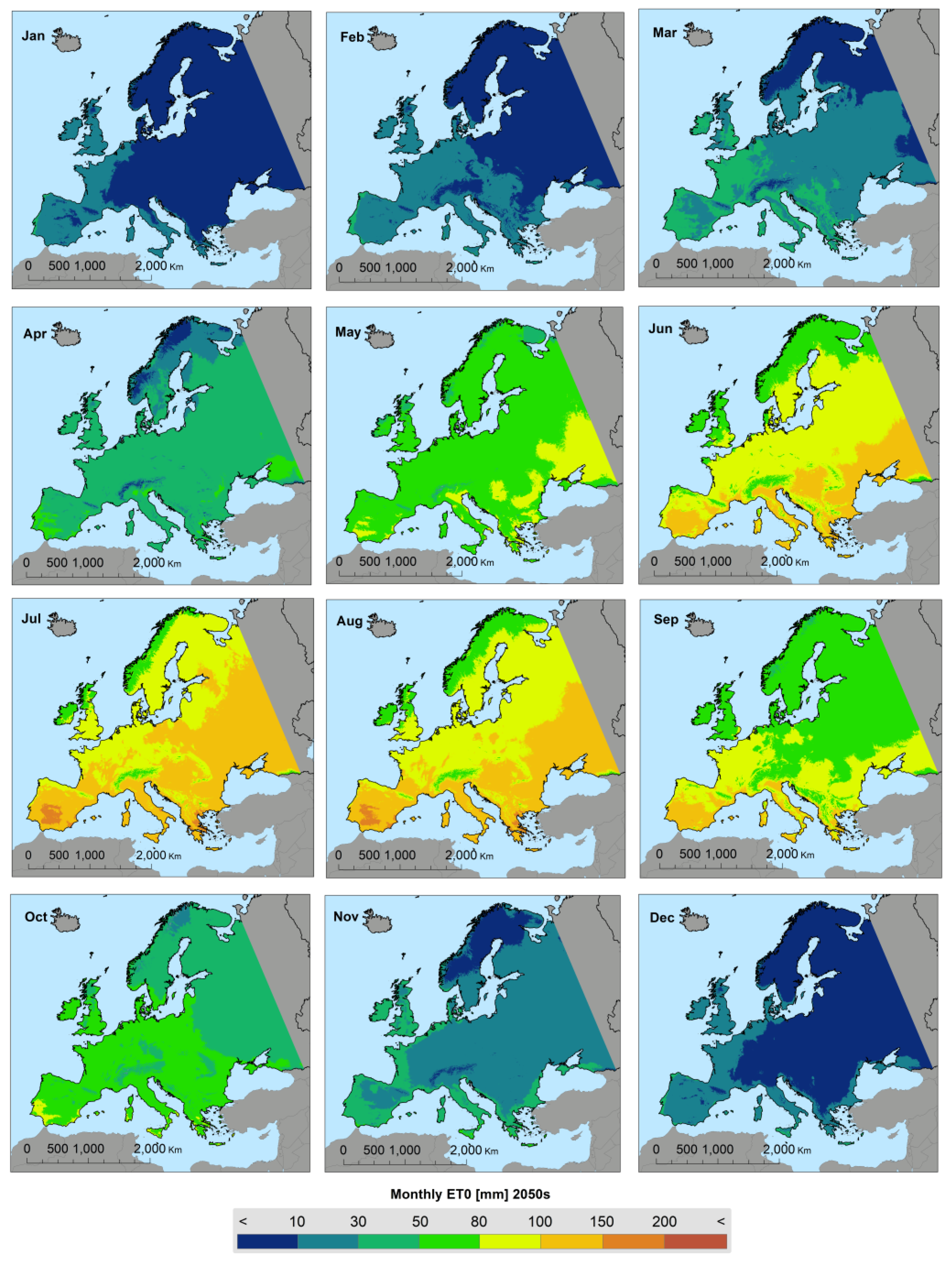
In the 2020s, the monthly ET0 varies from 0 mm to 280 mm, showing higher values during July and August but also in June and September following the increase in evapotranspiration as better evidenced on a larger spatial scale. The months with lower ET0 are January, February, March, November and December. Figure 5 reports the monthly ET0 in Europe during the 2020s. The monthly ET0 during the 2050s varies from 0 mm to 320 mm in the summer months of June, July and August, but also in September. The months with a lower ET0 are January, February, and December. Figure 6 illustrates the monthly ET0 in Europe during the 2050s.

It is important to notice that increases in the value of monthly ET0 were identified mostly in the summertime months of June, July, and August as well as during May and November during the 1990s, the 2020s, and the 2050s. The spatial distribution of the monthly ET0 shows major changes in Southern, Eastern and Western Europe. Minor changes were identified in the months of January and December during the three periods, with non-significant spatial changes in the North of Europe and in the mountainous areas.

4.2. Variation of AET0 over Europe

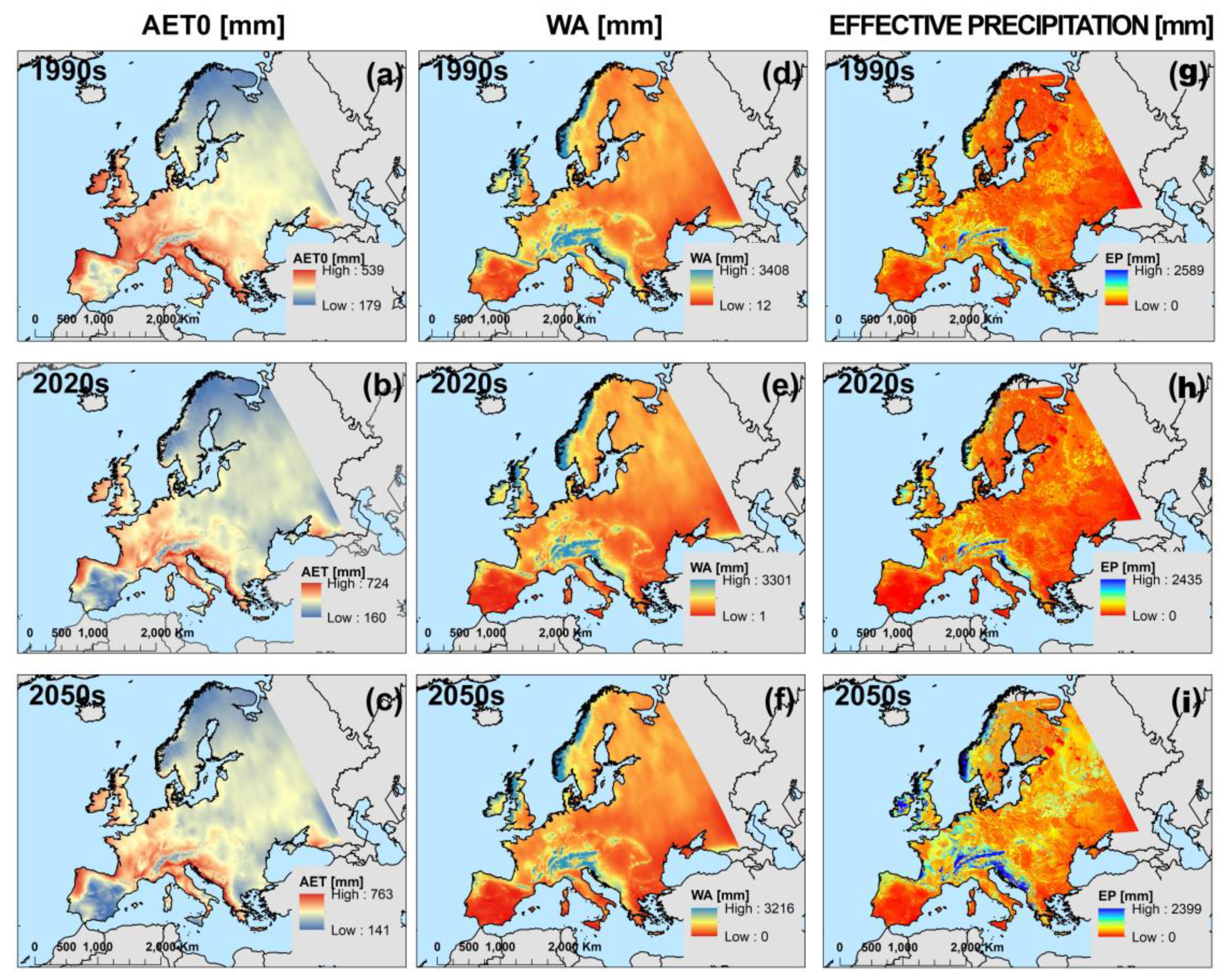
The spatial variation of AET0 across Europe during the three analyzed periods is shown in Figure 7a–c. The AET0 varied from 179 mm to 539 mm during 1990s and varies from 160 mm to 724 mm during the 2020s, and from 141 mm to 763 mm during the 2050s. The highest values of AET0 are found in the central part of Europe, in the Italian Peninsula, in the British Islands, in the North of the Iberian Peninsula, on the Dalmatian Coast and West Balkan Peninsula. The lowest AET0 values were found in the North of Europe, high mountains areas, and South of the Iberian Peninsula. Higher AET0 values reveal areas with high temperature values and higher values of precipitation while lower AET0 values evidence areas characterized by low values of both temperature and precipitation.

4.3. Variation of Water Availability (WA) and Effective Precipitation (EP)

The WA in Europe varied from 12 mm to 3408 mm in the 1990s (Figure 7d) and varies from 1 mm to 3101 mm during the 2020s (Figure 7e), and from 0 mm to 3216 mm during the 2050s (Figure 7f). The highest values of WA were found for the western Scandinavian Peninsula, the North of the British Isles, and over high mountains. The lowest values of WA were found in West, East, and Southern Europe.

The results show that effective precipitation in Europe varied from 0 mm to 2589 mm during the 1990s (Figure 7g). During the 2020s, the effective precipitation varies from 0 mm to 2435 mm (Figure 7h) while during the 2050s the effective precipitation will vary from 0 mm to 2399 mm (Figure 7i). The effective precipitation shows higher values in the mountainous areas (e.g., Alps Mountains, Dinaric Mountains), British Islands, and western Scandinavian Peninsula. As observed, the spatial distribution of effective precipitation with high values is directly influenced by low AET0 values and higher WA values in all three periods, but also by the PIMs which have higher PIC in mountainous areas with limestone.

5. Discussion

The main goal of this paper was to calculate and assess the spatial and temporal variation of actual evapotranspiration, water availability and effective precipitation over the European continent in three major periods. At the same time, the aim of the work was to come up with the high-resolution grid maps of these parameters, which are very significant for water resources evaluation and also for several studies.

The maps prepared in this work can be very useful for hydrology, climatology, geotechnical investigations, and civil engineering surveys, but also for environmental studies and resource planning. In this sense, the AET0 and WA are useful data for agriculture and irrigation planning during summer periods. The WA datasets also act as an important parameter for human needs and practices, for example in industry and domestic demands. The effective precipitation is more closely related to research and civil-engineering purposes. Thus, the effective precipitation datasets provide essential data required in the study of landslides and slope stability [43,45]. For instance, civil engineers use specialized software and models (e.g., Transient Rainfall Infiltration and Grid-Based Regional Slope-Stability Model TRIGRS) [46] and Scoops 3D is widely used for the determination of slope stability with spatial scale datasets [47]. In this sense, the variations in water availability and effective precipitation will have an impact on the groundwater table and a further effect on unsaturated soils [48].

The findings and maps are very useful inputs for various applications, mainly due to the climate impact on water resources in Europe. For the 1990s, 2020s and 2050s, it was shown that monthly ET0 will increase by 30% and the annual AET0 will increase by 40%, which implies a reduction in runoff and water availability. These changes are due to the temperature increases and slight decreases in precipitation projected for the future period.

Our work is not without limitations. First of all, we conducted a long-term period analysis of large study area, i.e., the European continent. Reliable results can be obtained for studies at the continental and regional scales, but for small areas of less than 1 km² the calculated parameters have similar values. Secondly, the frame of the analysis provides 30-year averages, which is convenient for the evaluation of climate and water resources over several decades and to develop future perspectives and plans. Another limitation is related to the monthly ET0 calculated using the Thornthwaite method, which is based on the temperature and precipitations parameters [49,50]. In this approach, the wind speed, solar radiation, and humidity were not considered due to a lack of data and also due to the uncertainties that may appear if these data are projected for the future. When applying this method, the value of monthly ET0 is underestimated mainly during the summer periods when the solar radiation is higher than in the winter for the Europe continent. Overall, the climate models support and homogenize the results at the continental scale, considering the downscaled and spatially customizable climate data [51]. For the European continent, the climate models were carried out from about 5000 meteorological climate stations and the results of temperature and precipitations are highly accurate [35]. In the South-East of Europe, the climate effect on groundwater resources was evaluated using similar climate models to those included in this paper [52].

In terms of short-time period analyses and modelling, a finer temporal resolution, e.g., hourly data, could improve the studies. However, the present work and grid datasets are a good point for the European continent and they show a holistic vision regarding the variation of climate parameters, water availability, and effective precipitation.

6. Conclusions

The original maps of AET0, WA, and effective precipitation over Europe were prepared in this study for the 1990s, 2020s, and 2050s at a 1 km² spatial resolution. Climate models of temperature and precipitation, geological information, and terrain data were the main datasets used here for the calculations. As the main focus, the AET0, WA, and effective precipitation datasets were performed in ArcGIS and all layers represent cartographical support for water resource investigations and future forecasts for drought, flooding and water demand for the European continent.

The main findings indicate a reduction in monthly ET0 by 30% between past and future periods. The variation of annual AET0 indicates decreases of up to 40% for the 2050s. These aspects will directly influence the variation in WA and EP, which are expected to decrease by 10% in the future. The areas with major impacts and WA and EP reduction include the Iberian Peninsula, Mediterranean areas, and Eastern Europe.

The homogenized grid datasets can be efficiently used together with the monitoring data to run the numerical analyses for drawing the hazard maps under different unsaturated conditions. To support the development of climate-change mitigation planning for water and natural resource management, we provide gridded data layers in the open access database (https://zenodo.org/record/5899476#.YfZBvOpByUk; doi: 10.5281/zenodo.5899476, accessed on 1 February 2022).

One of the strengths of the calculated datasets is the temporal frame whose perspective is of great interest for both the scientific community and authorities of each European country. The output of this work is basic support for future mid-century environmental planning. The technical validation of the present methods and output data rely on the body of previous publications [32,33].

References

- Haidu, I.; Nistor, M.M. Long-term effect of climate change on groundwater recharge in the Grand Est region, France. Meteorol. Appl. 2019, 27, e1796. [Google Scholar] [CrossRef] [Green Version]
- Galleani, L.; Vigna, B.; Banzato, C.; Lo Russo, S. Validation of a Vulnerability Estimator for Spring Protection Areas: The VESPA index. J. Hydrol. 2011, 396, 233–245. [Google Scholar] [CrossRef]
- Čenčur Curk, B.; Cheval, S.; Vrhovnik, P.; Verbovšek, T.; Herrnegger, M.; Nachtnebel, H.P.; Marjanović, P.; Siegel, H.; Gerhardt, E.; Hochbichler, E.; et al. CC-WARE Mitigating Vulnerability of Water Resources under Climate Change. WP3—Vulnerability of Water Resources in SEE, Report Version 5. 2014. Available online: https://www.ccware.eu/output-documentation/output-wp3.html (accessed on 1 February 2022).
- Nistor, M.M.; Dezsi, S.; Cheval, S. Vulnerability of groundwater under climate change and land cover: A new spatial assessment method applied on Beliş district (Western Carpathians, Romania). Environ. Eng. Manag. J. 2015, 14, 2959–2971. [Google Scholar]
- Aguilera, H.; Murillo, J.M. The effect of possible climate change on natural, groundwater recharge based on a simple model: A study of four karstic aquifers in SE Spain. Environ. Geol. 2009, 57, 963–974. [Google Scholar] [CrossRef]
- Kløve, B.; Ala-Aho, P.; Bertrand, G.; Gurdak, J.J.; Kupfersberger, H.; Kværner, J.; Muotka, T.; Mykrä, H.; Preda, E.; Rossi, P.; et al. Climate change impacts on groundwater and dependent ecosystems. J. Hydrol. 2014, 518, 250–266. [Google Scholar] [CrossRef]
- Jiménez Cisneros, B.E.; Oki, T.; Arnell, N.W.; Benito, G.; Cogley, J.G.; Döll, P.; Jiang, T.; Mwakalila, S.S. Freshwater Resources; Field, C.B., Barros, V.R., Dokken, D.J., Mach, K.J., Mastrandrea, M.D., Bilir, T.E., Chatterjee, M., Ebi, K.L., Estrada, Y.O., Genova, R.C., et al., Eds.; Climate Change 2014: Impacts, Adaptation, and Vulnerability. Part A: Global and Sectoral Aspects. Contribution of Working Group II to the Fifth Assessment Report of the Intergovernmental Panel on Climate Change; Cambridge University Press: Cambridge, UK; New York, NY, USA, 2014; pp. 229–269. Available online: http://ipcc-wg2.gov/AR5/report/full-report/ (accessed on 1 February 2022).
- Yan, Y.; Zhou, J.; He, Z.; Sun, Q.; Fei, J.; Zhou, X.; Zhao, K.; Yang, L.; Long, H.; Zheng, H. Evolution of Luyang Lake since the last 34,000 years: Climatic changes and anthropogenic impacts. Quat. Int. 2017, 440, 90–98. [Google Scholar] [CrossRef]
- Ghazavi, R.; Ebrahimi, Z. Assessing groundwater vulnerability to contamination in an arid environment using DRASTIC and GOD models. Int. J. Environ. Sci. Technol. 2015, 12, 2909–2918. [Google Scholar] [CrossRef] [Green Version]
- Nistor, M.M.; Nicula, A.S.; Cervi, F.; Man, T.C.; Irimuş, I.A.; Surdu, I. Groundwater vulnerability GIS models in the Carpathian Mountains under climate and land cover changes. Appl. Ecol. Environ. Res. 2018, 16, 5095–5116. [Google Scholar] [CrossRef]
- Stempvoort, D.V.; Ewert, L.; Wassenaar, L. Aquifers vulnerability index: A GIS—Compatible method for groundwater vulnerability mapping. Can. Water. Resour. J. 1993, 18, 25–37. [Google Scholar] [CrossRef] [Green Version]
- IPCC. Climate change 2001: The scientific basis. In Contribution of Working Group I to the Third Assessment Report of the Intergovernmental Panel on Climate Change; Houghton, J.T., Ding, Y., Griggs, D.J., Noguer, M., van der Linden, P.J., Dai, X., Eds.; Cambridge University Press: Cambridge, UK; New York, NY, USA, 2001; 881p. [Google Scholar]
- Stocks, B.J.; Fosberg, M.A.; Lynham, T.J.; Mearns, L.; Wotton, B.M.; Yang, Q.; Jin, J.Z.; Lawrence, K.; Hartley, G.R.; Mason, J.A.; et al. Climate change and forest fire potential in Russian and Canadian boreal forests. Clim. Change 1998, 38, 1–13. [Google Scholar] [CrossRef]
- Shaver, G.R.; Canadell, J.; Chapin, F.S.; Gurevitch, J.; Harte, J.; Henry, G.; Ineson, P.; Jonasson, S.; Melillo, J.; Pitelka, L.; et al. Global warming and terrestrial ecosystems: A conceptual framework for analysis. BioScience 2000, 50, 871–882. [Google Scholar] [CrossRef]
- Stavig, L.; Collins, L.; Hager, C.; Herring, M.; Brown, E.; Locklar, E. The Effects of Climate Change on Cordova, Alaska on the Prince William Sound. Alaska Tsunami Papers, The National Ocean Sciences Bowl. 2005. Available online: https://seagrant.uaf.edu/nosb/papers/2005/cordova-nurds.html (accessed on 1 February 2022).
- The Canadian Centre for Climate Modelling and Analysis. The First Generation Coupled Global Climate Model Publishing Web. 2014. Available online: http://www.ec.gc.ca/ccmac-cccma/default.asp?lang=En&n=540909E4-1 (accessed on 1 February 2022).
- Kargel, J.S.; Abrams, M.J.; Bishop, M.P.; Bush, A.; Hamilton, G.; Jiskoot, H.; Kääb, A.; Kieffer, H.H.; Lee, E.M.; Paul, F.; et al. Multispectral imaging contributions to global land ice measurements from space. Remote Sens. Environ. 2005, 99, 187–219. [Google Scholar] [CrossRef]
- Oerlemans, J. Extracting a Climate Signal from 169 Glacier Records. Science 2005, 308, 675–677. [Google Scholar] [CrossRef] [PubMed] [Green Version]
- Shahgedanova, M.; Stokes, C.R.; Gurney, S.D.; Popovnin, V. Interactions between mass balance, atmospheric circulation, and recent climate change on the Djankuat Glacier, Caucasus Mountains, Russia. J. Geophys. Res. 2005, 110, 1–12. [Google Scholar] [CrossRef]
- Dong, P.; Wang, C.; Ding, J. Estimating glacier volume loss used remotely sensed images, digital elevation data, and GIS modelling. Int. J. Remote. Sens. 2013, 34, 8881–8892. [Google Scholar] [CrossRef]
- Xie, X.; Li, Y.X.; Li, R.; Zhang, Y.; Huo, Y.; Bao, Y.; Shen, S. Hyperspectral characteristics and growth monitoring of rice (Oryza sativa) under asymmetric warming. Int. J. Remote Sens. 2013, 34, 8449–8462. [Google Scholar] [CrossRef]
- Elfarrak, H.; Hakdaoui, M.; Fikri, A. Development of Vulnerability through the DRASTIC Method and Geographic Information System (GIS) (Case Groundwater of Berrchid), Morocco. J. Geogr. Inf. Syst. 2014, 6, 45–58. [Google Scholar] [CrossRef] [Green Version]
- Nistor, M.M.; Petcu, I.M. Quantitative analysis of glaciers changes from Passage Canal based on GIS and satellite images, South Alaska. Appl. Ecol. Environ. Res. 2015, 13, 535–549. [Google Scholar]
- Yan, B.; Fang, N.F.; Zhang, P.C.; Shi, Z.H. Impacts of land use change on watershed streamflow and sediment yield: An assessment using hydrologic modelling and partial least squares regression. J. Hydrol. 2013, 484, 26–37. [Google Scholar] [CrossRef]
- Collins, D.N. Climatic warming, glacier recession and runoff from alpine basins after the little ice age maximum. Ann. Glaciol. 2008, 48, 119–124. [Google Scholar] [CrossRef] [Green Version]
- Hidalgo, H.G.; Das, T.; Dettinger, M.D.; Cayan, D.R.; Pierce, D.W.; Barnett, T.P.; Bala, G.; Mirin, A.; Wood, A.W.; Bonfils, C.; et al. Detection and attribution of streamflow timing changes to climate change in the western United States. J. Clim. 2009, 22, 3838–3855. [Google Scholar] [CrossRef]
- Nistor, M.M.; Man, T.C.; Benzaghta, M.A.; Nedumpallile Vasu, N.; Dezsi, S.; Kizza, R. Land cover and temperature implications for the seasonal evapotranspiration in Europe. Geogr. Tech. 2018, 13, 85–108. [Google Scholar] [CrossRef] [Green Version]
- Kottek, M.; Grieser, J.; Beck, C.; Rudolf, B.; Rubel, F. World Map of the Köppen-Geiger climate classification updated. Meteorol. Z. 2006, 15, 259–263. [Google Scholar] [CrossRef]
- Hamann, A.; Wang, T.; Spittlehouse, D.L.; Murdock, T.Q. A comprehensive, high-resolution database of historical and projected climate surfaces for western North America. Bull. Am. Meteorol. Soc. 2013, 94, 1307–1309. [Google Scholar] [CrossRef]
- IPCC. Summary for Policymakers. In Climate Change 2013: The Physical Science Basis. Contribution of Working Group I to the Fifth Assessment Report of the Intergovernmental Panel on Climate Change; Stocker, T.F., Qin, D., Plattner, G.-K., Tignor, M., Allen, S.K., Boschung, J., Nauels, A., Xia, Y., Bex, V., Midgley, P.M., Eds.; Cambridge University Press: Cambridge, UK; New York, NY, USA, 2013; 1308p. [Google Scholar]
- BGR & UNESCO. International Hydrogeological Map of Europe (IHME1500) 1:1,500,000. International Association of Hydrogeologists. 2013. Available online: http://www.bgr.bund.de/ihme1500/ (accessed on 1 February 2022).
- Rahardjo, H.; Satyanaga Nio, A.; Leong, E.C.; Song, N.Y. Effects of Groundwater Table Position and Soil Properties on Stability of Slope during Rainfall. J. Geotech. Geoenviron. Eng. 2010, 136, 1555–1564. [Google Scholar] [CrossRef]
- Haidu, I.; Nistor, M.M. Groundwater vulnerability assessment in the Grand Est region, France. Quat. Int. 2020, 547, 86–100. [Google Scholar] [CrossRef]
- Thornthwaite, C.W. An approach toward a rational classification of climate. Geogr. Rev. 1948, 38, 55–94. [Google Scholar] [CrossRef]
- Dezsi, S.; Mîndrescu, M.; Petrea, D.; Rai, K.P.; Hamann, A.; Nistor, M.M. High-resolution projections of evapotranspiration and water availability for Europe under climate change. Int. J. Climatol. 2018, 38, 3832–3841. [Google Scholar] [CrossRef]
- Nistor, M.M. Projection of annual crop coefficients in Italy based on climate models and land cover data. Geogr. Tech. 2018, 13, 97–113. [Google Scholar] [CrossRef]
- Nistor, M.M.; Cervi, F. Downscaling Budyko equation for monthly actual evapotranspiration estimation over the Emilia-Romagna region. Geogr. Tech. 2020, 15, 72–83. [Google Scholar] [CrossRef]
- Budyko, M.I. Climate and Life; Academic Press: New York, NY, USA, 1974. [Google Scholar]
- Gerrits, A.M.J.; Savenije, H.H.G.; Veling, E.J.M.; Pfister, L. Analytical derivation of the Budyko curve based on rainfall characteristics and a simple evaporation model. Water Resour. Res. 2009, 45, 1–15. [Google Scholar] [CrossRef]
- Nistor, M.M.; Mîndrescu, M. Climate change effect on groundwater resources in Emilia-Romagna region: An improved assessment through NISTOR-CEGW method. Quat. Int. 2019, 504, 214–228. [Google Scholar] [CrossRef]
- Cianflone, G.; Dominici, R.; Viscomi, A. Potential recharge estimation of the Sibari plain aquifers (Southern Italy) through a new GIS procedure. Geogr. Tech. 2015, 10, 8–18. [Google Scholar]
- Nistor, M.M. Groundwater vulnerability in Europe under climate change. Quat. Int. 2019, 547, 185–196. [Google Scholar] [CrossRef]
- Kim, Y.; Rahardjo, H.; Nistor, M.M.; Satyanaga, A.; Leong, E.C.; Sham, A.W.L. Assessment of critical rainfall scenarios for slope stability analyses based on historical rainfall records in Singapore. Environ. Earth Sci. 2022, 81, 39. [Google Scholar] [CrossRef]
- Russo, T.A.; Fisher, A.T.; Lockwood, B.S. Assessment of Managed Aquifer Recharge Site Suitability Using a GIS and Modeling. Ground Water 2015, 53, 389–400. [Google Scholar] [CrossRef] [Green Version]
- Satyanaga, A.; Zhai, Q.; Rahardjo, H. Estimation of Unimodal Water Characteristic Curve for Gap-graded Soil. Soils Found. 2017, 57, 789–801. [Google Scholar] [CrossRef]
- Rahardjo, H.; Satyanaga, A. Sensing and monitoring for assessment of rainfall-induced slope failures in residual soil. Proc. Inst. Civ. Eng. Geotech. Eng. 2019, 172, 496–506. [Google Scholar] [CrossRef]
- Satyanaga, A.; Rahardjo, H.; Hua, C.J. Numerical Simulation of Capillary Barrier System under Rainfall Infiltration. ISSMGE Int. J. Geoeng. Case Hist. 2019, 5, 43–54. [Google Scholar] [CrossRef]
- Satyanaga, A.; Rahardjo, H. Role of Unsaturated Soil Properties in The Development of Slope Susceptibility Map. Proc. Inst. Civ. Eng. Geotech. Eng. 2020, 1–13. [Google Scholar] [CrossRef]
- Nistor, M.M.; Rai, P.K.; Carebia, I.A.; Singh, P.; Pratap Shahi, A.; Mishra, V.N. Comparison of the effectiveness of two Budyko-based methods for actual evapotranspiration in Uttar Pradesh, India. Geogr. Tech. 2020, 15, 1–15. [Google Scholar] [CrossRef]
- Pratoomchai, W.; Tantanee, S.; Ekkawatpanit, C. A comprehensive grid-based rainfall characteristics in the central plain river basin of Thailand. Geogr. Tech. 2020, 15, 47–56. [Google Scholar] [CrossRef]
- Wang, T.; Hamann, A.; Spittlehouse, D.L.; Carroll, C. Locally downscaled and spatially customizable climate data for historical and future periods for North America. PLoS ONE 2016, 11, e0156720. [Google Scholar] [CrossRef] [PubMed]
- Nistor, M.M. Climate change effect on groundwater resources in South East Europe during 21st century. Quat. Int. 2019, 504, 171–180. [Google Scholar] [CrossRef]
Figure 1.
Climate variables as input data in Europe and output results list. (a) Mean annual air temperature (TT) in 1990s. (b) Mean annual air temperature (TT) in 2020s. (c) Mean annual air temperature (TT) in 2050s. (d) Mean annual precipitation (PP) in 1990s. (e) Mean annual precipitation (PP) in 2020s. (f) Mean annual precipitation (PP) in 2050s.
Figure 2.
Framework of geology, terrain data, and potential infiltration map in Europe. (a) Geological formations map. (b) Digital elevation model. (c) Potential infiltration map (PIM). Note: Potential infiltration map was calculated as ratio of potential infiltration coefficient and normalization slope layer (radian degrees).
Figure 3.
Spatial distribution of Alfa parameter (α), heat index (I), and annual potential evapotranspiration (ET0) in Europe. (a) Alfa parameter α in 1990s. (b) Alfa parameter α in 2020s. (c) Alfa parameter α in 2050s. (d) Heat index I in 1990s. (e) Heat index I in 2020s. (f) Heat index I in 2050s. (g) Annual ET0 in 1990s. (h) Annual ET0 in 2020s. (i) Annual ET0 in 2050s.
Figure 4.
Spatial distribution of monthly ET0 over Europe during 1990s.
Figure 5.
Spatial distribution of monthly ET0 across Europe during 2020s.
Figure 6.
Spatial distribution of monthly ET0 over Europe during 2050s.
Figure 7.
Variables list as input data in Europe and output results including actual evapotranspiration, (AET0), water availability (WA), and effective precipitation. (a) Actual evapotranspiration AET0 in 1990s. (b) Actual evapotranspiration AET0 in 2020s. (c) Actual evapotranspiration AET0 in 2050s. (d) Water availability WA in 1990s. (e) Water availability WA in 2020s. (f) Water availability WA in 2050s. (g) Effective precipitation in 1990s. (h) Effective precipitation in 2020s. (i) Effective precipitation in 2050s.
Publisher’s Note: MDPI stays neutral with regard to jurisdictional claims in published maps and institutional affiliations. |
© 2022 by the authors. Licensee MDPI, Basel, Switzerland. This article is an open access article distributed under the terms and conditions of the Creative Commons Attribution (CC BY) license (https://creativecommons.org/licenses/by/4.0/).
Share and Cite
MDPI and ACS Style
Nistor, M.-M.; Satyanaga, A.; Dezsi, Ş.; Haidu, I. European Grid Dataset of Actual Evapotranspiration, Water Availability and Effective Precipitation. Atmosphere 2022, 13, 772. https://0-doi-org.brum.beds.ac.uk/10.3390/atmos13050772
AMA Style
Nistor M-M, Satyanaga A, Dezsi Ş, Haidu I. European Grid Dataset of Actual Evapotranspiration, Water Availability and Effective Precipitation. Atmosphere. 2022; 13(5):772. https://0-doi-org.brum.beds.ac.uk/10.3390/atmos13050772
Chicago/Turabian StyleNistor, Mărgărit-Mircea, Alfrendo Satyanaga, Ştefan Dezsi, and Ionel Haidu. 2022. "European Grid Dataset of Actual Evapotranspiration, Water Availability and Effective Precipitation" Atmosphere 13, no. 5: 772. https://0-doi-org.brum.beds.ac.uk/10.3390/atmos13050772
Note that from the first issue of 2016, this journal uses article numbers instead of page numbers. See further details here.