Article

Ongoing Decline in the Atmospheric COS Seasonal Cycle Amplitude over Western Europe: Implications for Surface Fluxes

Laboratoire des Sciences du Climat et de L’Environnement, UMR 8212 CEA-CNRS-UVSQ, Université Paris-Saclay, 91191 Gif-sur-Yvette, France
*
Author to whom correspondence should be addressed.
Submission received: 31 March 2022 / Revised: 12 May 2022 / Accepted: 14 May 2022 / Published: 16 May 2022
(This article belongs to the Section Biosphere/Hydrosphere/Land–Atmosphere Interactions)

Abstract

:
Atmospheric carbonyl sulfide (COS) was monitored at the GIF site (France) from August 2014 to November 2021. A significant decreasing trend in the seasonal cycle amplitude (SCA) of the COS was observed for the first time in the Northern Hemisphere (−27 ppt over 6 years). The lowest SCA was recorded in 2021 (80 ppt vs. 107 ppt in 2015). The trend in the SCA results revealed a steeper decline in the spring maximum than in that of the autumn minimum (−49 ppt vs. −10 ppt over 6 years, respectively). These negative trends were qualitatively consistent with those in the tropospheric COS put forward by the NDACC network of ground-based FTIR instruments, which were attributed to a slowing in the rate of COS anthropogenic emissions. Simulations using the ORCHIDEE land-surface model showed that a decrease in COS lowers the uptake of this gas by plants. Our observations suggest the existence of a causal relationship between the decline in the SCA and that in the tropospheric COS, implying that the temporal variations in the COS SCA over Western Europe are essentially driven by plant uptake. However, the transport by the LMDz 3-D model of surface fluxes for each component of the COS budget failed to reproduce this feature at GIF, pointing to a likely misrepresentation of the marine and anthropogenic fluxes in the footprint of this station.

1. Introduction

The uptake of atmospheric carbonyl sulfide (COS) by terrestrial vegetation is the major sink in the global budget of this gas [1]. Moreover, the plant uptake of COS has been recognized as a promising tracer of carbon dioxide (CO2) exchange during photosynthesis [2], also known as gross primary production (GPP). Thus, long-term atmospheric COS records, derived from ice-core, firn, and ambient air samples, as well as ground-based observations by solar-viewing Fourier transform interferometry (FTIR), were used by Campbell et al. (2018) to estimate the historical growth of global GPP [3]. Illustrations of the high potential of atmospheric COS measurements, carried out in the framework of the NOAA-ESRL network, were also provided by Parazoo et al. (2021) and Hu et al. (2021) to help understand the seasonal and spatial distribution of plant carbon uptake across the Eastern United States, and the atmospheric CO2 seasonal cycle amplification observed in the Arctic and boreal North America, respectively [4,5]. However, the Siberian and temperate ecosystems (particularly those of the Central and Eastern United States, and Southeastern Europe) shape the Northern Hemisphere’s CO2 seasonal amplification rather than the Arctic-boreal North American ecosystems [6]. Unfortunately, atmospheric COS mole fraction surface observations in the middle and high latitudes of Europe (i.e., Mace Head station (MHD, IE, 53.3° N [7]); Jungfraujoch station (CH, 46.5° N [8]); Lutjewad station (NL, 53.4° N [9]); Hyytiälä station (FI, 61.8° N [10]); Gif-sur-Yvette station (GIF, FR, 48.7° N [11])) are scarcer than over North America, comparability of data from different laboratories are not ensured, and airborne measurements are still in the early stages [12,13], which prevents the application of the approach of [5] to Europe. Note that nine out of thirteen FTIR stations, operated as part of the Network for Detection of Atmospheric Composition Change (NDACC) in the Northern Hemisphere north of 35°N, are located in Europe and Japan, and yet none are found in Siberia [14]. Although NDACC monitoring stations have proven their utility in assessing tropospheric long-term trends and the seasonality in COS [8,14,15], it is unlikely that trends in COS and CO2 seasonal cycle amplitude (SCA) could be assessed simultaneously with sufficient precision from NDACC retrievals, as the tropospheric CO2 signal (e.g., the SCA) is damped in comparison to Total Carbon Column Observing Network (TCCON) retrievals [16].
In their study, Hu et al. (2021) used atmospheric COS measurements collected essentially over North America between 2009 and 2013, a period during which a slight rise in COS was observed in the Northern Hemisphere (NH) by NDACC [14] and by NOAA ground stations [7], essentially because the year 2009 was anomalously low in this latter case (Figure 1). CO2 mole fractions exhibited a significant increase during this period (Figure 1).
Hence, during the 2009–2013 period, the change in the NH COS-to-CO2 ratio was very small (1.23 ± 0.01). An inflexion point was reached in 2013 (Figure 1). The trend in the NH COS-to-CO2 ratio is now driven by decreasing COS and continuously rising CO2.
In this paper, we address the implications for the COS surface fluxes of the trends observed in COS concentrations and SCA, in light of the recently updated COS time series at GIF (2014–2021). Moreover, simulations were performed using the ORCHIDEE land-surface model (LSM) and the LMDz global atmospheric transport model to evaluate our current understanding of the biogeochemistry of COS in Western Europe against field observations.

2. Materials and Methods

At the GIF monitoring site (48.7109 N, 2.1476 E), atmospheric COS was collected on an hourly basis from August 2014 to November 2021 using an Entech P7100 preconcentrator, and subsequently analyzed by gas chromatography (Varian Model 3800) with pulsed flame photometry detection (PFPD, [11,18]). The comparability of our own calibration scale supplied by Air Products with that of NOAA-2004 [7] was assessed on a weekly basis using two long-term natural air standards consecutively, which were prepared in Aculife-treated cylinders and calibrated by NOAA-ESRL [11]. The same long-term air standard was used during the first six years of our approximately seven-year long time series. The latter was interrupted for only about two months in summer 2017, due to a failure of the Entech preconcentrator, and in spring 2020, because of the COVID-19 lockdown. Fortunately, data collected by a second instrument (quantum cascade laser spectrometer, mini QCLS COS/CO2/H2O, Aerodyne Res.) operated at the Trainou (TRN, FR, 47.9647 N–2.1126 E) monitoring site, about 80 km south-west of GIF, was available to fill the 2020 data gap [19]. The reader is referred to [11] for a description of COS measurements by QCLS.
Post-processing of the COS measurements (selection of daytime (11–17 h UTC) data, calculation of the long-term trend and smoothing of the seasonal cycle, and calculation of the spring maximum and autumn minimum) used the CCGvu curve-fitting procedure developed by [20]. The procedure is fully described and available at http://www.esrl.noaa.gov/gmd/ccgg/mbl/crvfit/crvfit.html (accessed on 1 November 2021). The procedure first estimates a smoothing function by fitting the raw data to a first-order polynomial equation for the growth rate combined with a two-harmonics function for the annual cycle. In order to define short-term and long-term variations that are not captured by the function, the residuals (i.e., raw time series minus the full function) were fitted using a low-pass filter with 80 and 667 days as short-term and long-term cutoff values, respectively. The smooth curve combines the results of the function and of the filter using the short-term cutoff value. Detrended seasonal cycles were also calculated by subtracting the long-term trend (i.e., polynomial plus filtered residuals using the long-term cutoff value) to the smooth curve.
An offline version of LMDz 6 [21], based on the general circulation model developed at the Laboratoire de Météorologie Dynamique [22], was used to simulate atmospheric COS concentrations from fluxes described in other studies, discussed below. The LMDz grid features a 3.75°lon × 1.9°lat horizontal resolution and a 200–300 m vertical resolution in the planetary boundary layer, with 39 sigma-pressure layers from the surface to about 75 km. European Center for Medium-Range Weather Forecasts (ECMWF) fields are prescribed and pre-computed mass fluxes from the full LMDz version are used for the offline version, which only solves the continuity equation for the tracers. LMDz was run for the years 2010 to 2019 at a 30-min time step to simulate 3-hourly average outputs. The GIF station generally samples air masses from Central France and countries at the northeastern edge of France, such as Belgium, Germany and Switzerland, as shown by the LMDz footprints (see Figure S14 of [17]).
The ORCHIDEE LSM was used to simulate global vegetation and soil COS fluxes. ORCHIDEE is developed at the Institute Pierre Simon Laplace (IPSL) and computes the carbon, water, and energy balance between the land surfaces and the atmosphere. It was initially described in [23]. Plant species were grouped into 14 plant functional types (PFTs) based on similarities in morphology, phenology, climatic conditions, and photosynthetic pathways. A final PFT corresponded to bare soil. Each grid cell was divided into fractions of PFTs, with a distribution prescribed by yearly-varying PFT maps derived from the ESA Climate Change Initiative (CCI) land-cover products [24]. ORCHIDEE global simulations were forced with 0.5° and 6-hourly CRUJRA reanalysis [25]. The monthly near-surface atmospheric COS concentrations used for the computation of vegetation and soil COS fluxes were obtained from LMDz simulations forced with optimized COS surface fluxes [17]. ORCHIDEE global simulations were performed by running a 340-year spin-up simulation in fixed conditions to stabilize all carbon pools and to equilibrate the net biome production [26], followed by a transient phase simulation to introduce increasing CO2 concentrations, varying climate, and PFT distribution. Next, vegetation and soil COS fluxes were computed from 2000 to 2019 at a 0.5° spatial resolution following [27,28], respectively. Of central importance in the following is the plant COS uptake, which is based on [29], where the flux in COS uptake (FCOS) is the product of the background atmospheric COS mixing ratio (COS) and gT_COS, where gT_COS is the total of three conductances to COS, i.e., the boundary layer, stomatal, and internal conductances to COS. All fluxes from the different COS source and sink components are listed in Table 1; this global budget of COS is almost in balance (i.e., +19 GgS yr−1).
In addition, we conducted a sensitivity study of atmospheric COS to the spatio-temporal distribution and magnitude of the oceanic source of COS by comparing two datasets of oceanic fluxes, one from [31,32] and the optimized fluxes from [17]. After optimization, the total oceanic emissions account for 445 GgS yr−1 of the global budget of COS [17]. By jointly assimilating the surface measurements of COS and CO2 into LMDz, the authors of [17] were able to optimize some of the CO2 and COS budget components. In particular, [17] decreased the seasonal amplitude of the total COS oceanic fluxes in middle and high latitudes to match the observed NH concentrations at the NOAA-ESRL stations ALT, BRW, SUM, MHD, LEF, THD, and HFM. This amounts to stating that the oceanic emissions of COS presented in [31,32] during the boreal summer are overestimated in the middle and high latitudes.
Finally, because atmospheric transport is considered linear with respect to the surface fluxes in the model, each flux can be transported separately by the LMDz atmospheric transport model to simulate individual signal components, as shown later in dealing with the seasonality of COS. All simulated concentrations can be summed together to obtain the simulated concentrations of COS at sites GIF and MHD, represented by the “net” curves in those .

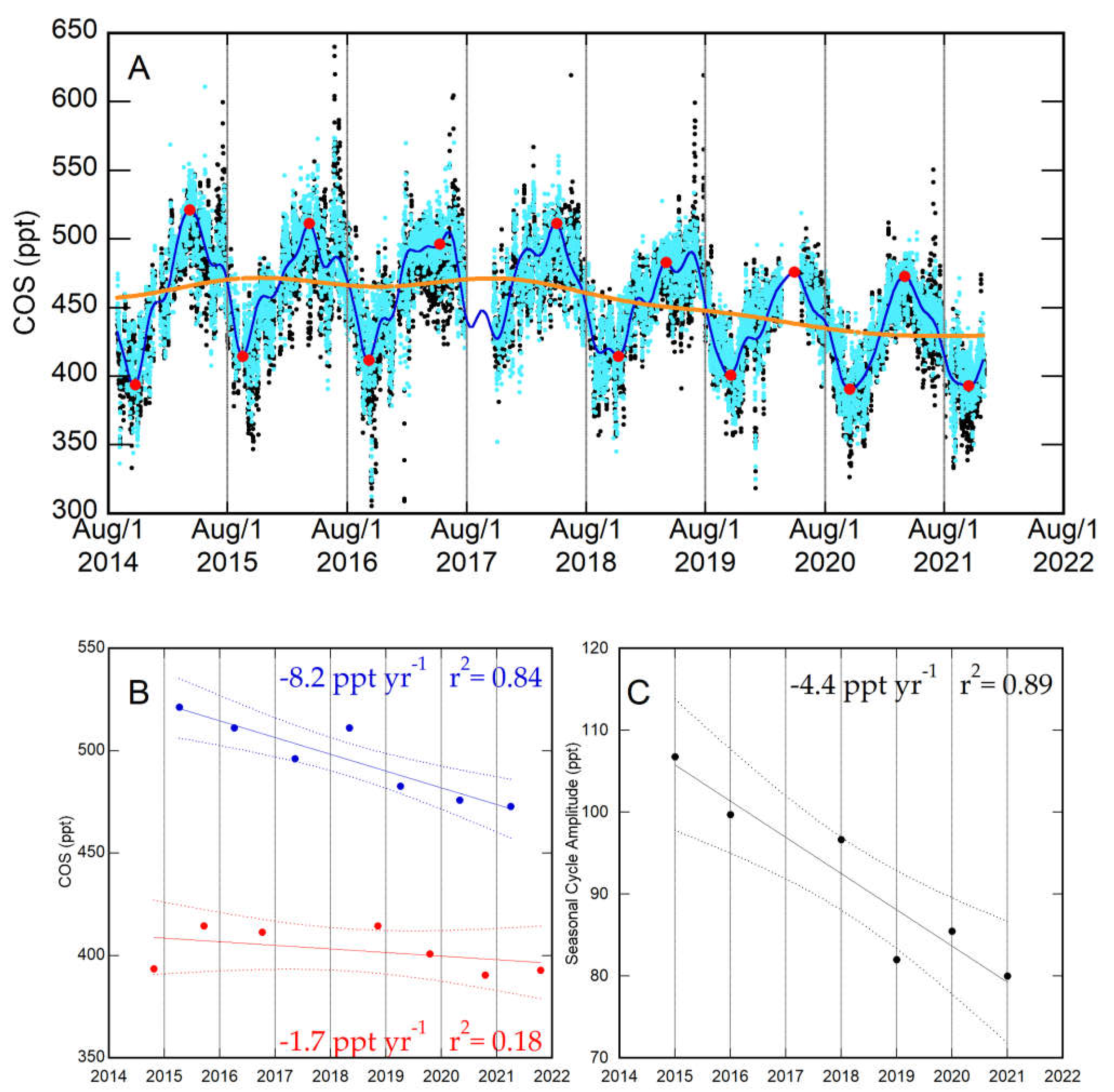
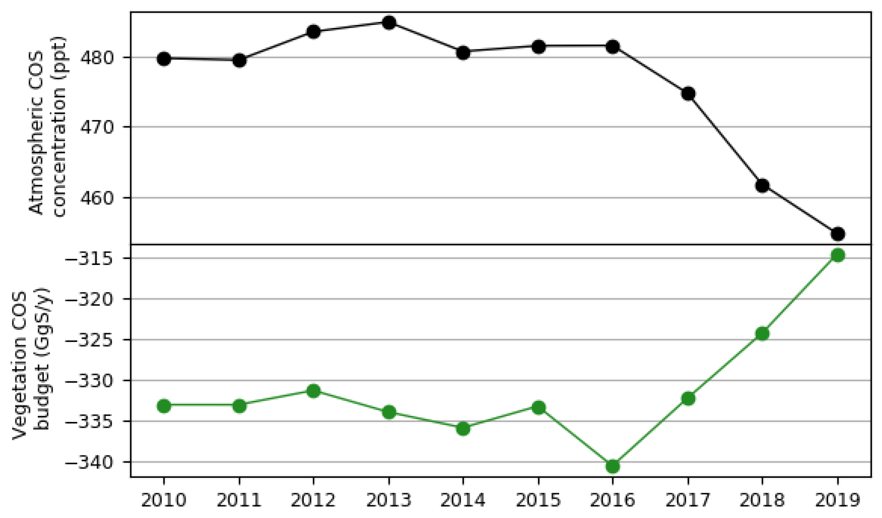
3. Results and Discussion

Figure 2A shows the temporal variations in the night-time and daytime COS mixing ratios, as well as the long-term and seasonal variations obtained from only considering the daytime data (n = 11,315 out of 46,860 data points) using the CCGvu curve-fitting procedure.
The spring maximum and the autumn minimum are depicted by a series of red dots. The relevant data for autumn 2017 are missing because no other instrument was operational during that time to fill the data gap. In other words, the CCGvu curve fitting realistically represents the magnitude of the springtime COS maximum of the year 2020, but not that of autumn 2017, because the daytime mixing ratios at the TRN site were proven not to have exceeded 500 ppt during the French lockdown due to the COVID-19 pandemic [19]. The daytime COS measurements show variability in seasonal and interannual timescales. The record undergoes a seasonal cycle with a peak in spring and a trough in autumn (Figure 2A). Note the presence in early summer of a shoulder on the fitting curve, which occasionally evolves into a secondary maximum. During this period, the COS enhancements are higher during night-time than daytime (Figure 2A). This is consistent with the existence of COS emissions from agroecosystems in late spring-–early summer, when wheat and rapeseed are grown within the footprint of the monitoring station [19], where nocturnal stability allows the accumulation of COS near the ground until vertical mixing recovers the next morning. Hence, to draw a distinction between the date of the spring maximum and that of the summer, we set May 15th as the upper limit for the detection of the spring maximum. The results also show that the spring maximum declined at a rate of −8.2 ppt/year (−49 ppt over 6 years). The autumn minimum showed a similar trend, although it was less steady and had a lower rate, of −1.7 ppt/year (−10 ppt over 6 years, Figure 2B). Intriguingly, the amplitude of the seasonal cycle at GIF decreased unsteadily from 2015, at a rate of −4.4 ppt yr−1, totaling −27 ppt over 6 years (Figure 2C). The lowest value in terms of magnitude of the spring maximum and SCA was recorded during the year 2021. Because the spring maximum and SCA both follow a clear decreasing trend over 6 years, it can be hypothesized that a causal relationship exists between the decrease in COS in the atmosphere and the reduction in the COS SCA through the role played by the biogenic sinks in the global budget of this gas. The rationale behind this hypothesis was tested with our model simulations.
Mechanistic soil and vegetation COS models have recently been implemented in the ORCHIDEE LSM [27,28]. The implementation of spatio-temporal variations in the near-surface atmospheric COS concentrations in the modeling of biogenic COS fluxes (Figure 3) helped reduce the imbalance of the atmospheric budget of this gas by lowering its uptake by soils and vegetation globally [28]. A reduction of about 8% in the vegetation uptake in the NH was simulated by the ORCHIDEE LSM between 2016 and 2019 (Figure 3).
The atmospheric COS at GIF followed a similar decreasing trend from 2019 onward (Figure 2A), leading to an apparent reduction in the simulated vegetation uptake of about 10% during the period of 2016–2021. As the dominant influence on the seasonal variation in the atmospheric COS is terrestrial vegetation uptake in the Northern Hemisphere, e.g., [36], the trends in the COS SCA and vegetation uptake were expected to evolve in parallel, as the observations and simulations at the GIF site suggest. A more quantitative appraisal of the sensitivity of the simulated tropospheric COS mixing ratio to the seasonal variability in the COS terrestrial fluxes is shown in the following. Using surface fluxes described in previous studies for each component of the COS budget (Table 1) and the LMDz transport model, the results indicate that the COS seasonality at GIF is characterized by two offsetting components from plant uptake and ocean emissions, regardless of the selected time period (Figure 4A,C). Consequently, the transport of anthropogenic emissions imposes the overall seasonality of the COS concentrations modeled at the GIF site, even though the observations lag the net signal by 2 to 4 months.
The Irish site of Mace Head (MHD), which faces the Atlantic Ocean, is the sole site belonging to NOAA’s network of COS monitoring stations in Europe. It is a marine regional reference, and MHD can be considered upwind of GIF. At MHD, the simulated net signal appears to be essentially driven by ocean fluxes, with the simulated seasonal maximum and minimum delayed by 2 to 3 months compared to the observations, regardless of the selected time period (Figure 4B,D). Note that although the GIF and MHD sites exhibit the same seasonality in terms of phase and amplitude (compare the grey dashed lines in Figure 4), the latter was driven within our modeling framework by distinct processes. It is suggested that this discrepancy likely results from errors in the seasonal cycle in the ocean emissions because a better fit between simulations and observations is observed at MHD when an optimized marine source is adopted (compare the grey dashed line and the black line in Figure S1B,D).
Other key features of the GIF COS time series are the 2015–2021 declining trend (Figure 2A, orange curve) and that in the spring maximum of COS (Figure 2B, blue line), both of which qualitatively agree with NOAA’s observations (Figure 1). In their global atmospheric COS trend analysis from 22 NDACC stations, the authors of [14] reach the conclusion that a slowing down in the rate of anthropogenic emissions is likely the cause of the recent (i.e., from 2016 to 2020) negative trends in free troposphere (FT) COS because, during the building phase of the COS between 1986–2012, the FT COS showed a high correlation with the revised anthropogenic emissions budget described in [31]. Although our multi-year observations are consistent with Hannigan’s conclusion as to the role played by anthropogenic emissions in the recent negative trends in tropospheric COS, the discrepancies between the observed and simulated seasonal variations at the MHD and GIF sites (Figure 4 and Figure S1) point to a likely misrepresentation of the marine and anthropogenic surface fluxes in the footprint of the latter.

4. Conclusions

The Gif-sur-Yvette time series (August 2014 to November 2021), made of 46,860 hourly measurements of the atmospheric COS mixing ratio carried out at 7 m above ground level, was analyzed for significant trends in seasonal to multi-year scales. These long-term measurements provided critical constraints on the budget of the COS in the footprint area of the GIF station. The daytime spring maximum and the seasonal cycle amplitude (SCA) exhibited decreasing trends during the 2015–2021 time period. This points to a causal relationship, implying that the SCA is essentially driven by the COS plant uptake in response to changes in the atmospheric background of this gas, as the ORCHIDEE and other land-surface models show. However, when previously documented surface fluxes were transported using the LMDz atmospheric transport model, the simulated and observed seasonal variations in the COS exhibited large discrepancies in terms of amplitude and phase. This points to a likely misrepresentation of the marine and anthropogenic surface fluxes in the footprint area of the GIF site. We look forward to the performance of a more accurate model simulation to represent the marine and anthropogenic components with, in this latter case, particular attention paid to the emissions from the most recent decade, which are yet to be inventoried.

Supplementary Materials

The following supporting information can be downloaded at: https://0-www-mdpi-com.brum.beds.ac.uk/article/10.3390/atmos13050812/s1. Figure S1: Simulations of the mean seasonal cycle of tropospheric COS mixing ratios over the years 2011–2015 (left column, NH mean annual atmospheric COS concentration in the range 483.7–491.5 ppt) and 2016–2019 (right column, decreasing NH mean annual atmo-spheric COS concentration in the range 486.9–467.8 ppt, see Figure 3) at the GIF (A,C) and MHD (B,D) monitoring stations. These simulations only account for the first-order relationship between the COS plant/soil fluxes and NH mean annual atmospheric COS concentrations. The net signal (black line) was obtained from a global LMDz simulation using all the dominant sources and sinks, while the signal components (colored lines) were obtained by running the global atmospheric simulation with one component flux at a time. Observations are shown in grey (dashed line). Here, optimized marine emissions (cf., Figure 4) were used instead of the standard ones.

Author Contributions

Conceptualization, methodology, data curation, writing—original draft preparation, S.B., M.R. (Marine Remaud), and C.A.; software, M.R. (Marine Remaud) and C.A.; writing—review and editing, F.M., M.R. (Michel Ramonet), and P.P.; visualization, S.B., M.R. (Marine Remaud), and C.A. All authors have read and agreed to the published version of the manuscript.

Funding

This research received no external funding.

Institutional Review Board Statement

Not applicable, studies not involving humans or animals.

Informed Consent Statement

Not applicable.

Data Availability Statement

Data supporting reported results can be found at https://0-doi-org.brum.beds.ac.uk/10.14768/6800b065-dcec-4006-ada5-b5f62a4bb832 (accessed on 24 March 2022).

Acknowledgments

The authors thank the three reviewers for their constructive and useful comments, which helped to further improve this study. We also acknowledge Sinikka T. Lennartz for providing the oceanic flux data.

Conflicts of Interest

The authors declare no conflict of interest.

References

  1. Whelan, M.E.; Lennartz, S.T.; Gimeno, T.E.; Wehr, R.; Wohlfahrt, G.; Wang, Y.; Kooijmans, L.M.J.; Hilton, T.W.; Belviso, S.; Peylin, P.; et al. Reviews and syntheses: Carbonyl sulfide as a multi-scale tracer for carbon and water cycles. Biogeosciences 2018, 15, 3625–3657. [Google Scholar] [CrossRef] [Green Version]
  2. Keeling, R.F.; Graven, H.D. Insights from time series of atmospheric carbon dioxide and related tracers. Annu. Rev. Environ. Resour. 2021, 46, 85–110. [Google Scholar] [CrossRef]
  3. Campbell, J.E.; Berry, J.A.; Seibt, U.; Smith, S.J.; Montzka, S.A.; Launois, T.; Belviso, S.; Bopp, L.; Laine, M. Large historical growth in global terrestrial gross primary production. Nature 2017, 544, 84–87. [Google Scholar] [CrossRef] [PubMed]
  4. Parazoo, N.C.; Bowman, K.W.; Baier, B.C.; Liu, J.; Lee, M.; Kuai, L.; Shiga, Y.; Baker, I.; Whelan, M.E.; Feng, S.; et al. Covariation of airborne biogenic tracers (CO2, COS, and CO) supports stronger than expected growing season photosynthetic uptake in the southeastern US. Glob. Biogeochem. Cycles 2021, 35, 1–23. [Google Scholar] [CrossRef]
  5. Hu, L.; Montzka, S.A.; Kaushik, A.; Andrews, A.E.; Sweeney, C.; Miller, J.; Baker, I.T.; Denning, S.; Campbell, E.; Shiga, Y.P.; et al. COS-derived GPP relationships with temperature and light help explain high-latitude atmospheric CO2 seasonal cycle amplification. Proc. Natl. Acad. Sci. USA 2021, 118, 1–10. [Google Scholar] [CrossRef]
  6. Lin, X.; Rogers, B.M.; Sweeney, C.; Chevallier, F.; Arshinov, M.; Dlugokencky, E.; Machida, T.; Sasakawa, M.; Tans, P.; Keppel-Aleks, G. Siberian and temperate ecosystems shape Northern Hemisphere atmospheric CO2 seasonal amplification. Proc. Natl. Acad. Sci. USA 2020, 117, 21079–21087. [Google Scholar] [CrossRef]
  7. Montzka, S.A.; Calvert, P.; Hall, B.D.; Elkins, J.W.; Conway, T.J.; Tans, P.P.; Sweeney, C. On the global distribution, seasonality, and budget of atmospheric carbonyl sulfide (COS) and some similarities to CO2. J. Geophys. Res. Atmos. 2017, 112, D09302. [Google Scholar] [CrossRef]
  8. Lejeune, B.; Mahieu, E.; Vollmer, M.K.; Reimann, S.; Bernath, P.F.; Boone, C.D.; Walker, K.A.; Servais, C. Optimized approach to retrieve information on atmospheric carbonyl sulfide (OCS) above the Jungfraujoch station and change in its abundance since 1995. J. Quant. Spectrosc. Radiat. Transf. 2016, 186, 81–95. [Google Scholar] [CrossRef]
  9. Kooijmans, L.M.J.; Uitslag, N.A.M.; Zahniser, M.S.; Nelson, D.D.; Montzka, S.A.; Chen, H. Continuous and high-precision atmospheric concentration measurements of COS, CO2, CO and H2O using a quantum cascade laser spectrometer (QCLS). Atmos. Meas. Tech. 2016, 9, 5293–5314. [Google Scholar] [CrossRef] [Green Version]
  10. Kooijmans, L.M.J.; Maseyk, K.; Seibt, U.; Sun, W.; Vesala, T.; Mammarella, I.; Kolari, P.; Aalto, J.; Franchin, A.; Vecchi, R.; et al. Canopy uptake dominates nighttime carbonyl sulfide fluxes in a boreal forest. Atmos. Chem. Phys. 2017, 17, 11453–11465. [Google Scholar] [CrossRef] [Green Version]
  11. Belviso, S.; Lebegue, B.; Ramonet, M.; Kazan, V.; Pison, I.; Berchet, A.; Delmotte, M.; Yver-Kwok, C.; Montagne, D.; Ciais, P. A top-down approach of sources and non-photosynthetic sinks of carbonyl sulfide from atmospheric measurements over multiple years in the Paris region (France). PLoS ONE 2020, 15, 0228419. [Google Scholar] [CrossRef] [PubMed] [Green Version]
  12. Kloss, C.; Tan, V.; Leen, J.B.; Madsen, G.L.; Gardner, A.; Du, X.; Kulessa, T.; Schillings, J.; Schneider, H.; Schrade, S.; et al. Airborne Mid-Infrared Cavity enhanced Absorption spectrometer (AMICA). Atmos. Meas. Tech. 2021, 14, 5271–5297. [Google Scholar] [CrossRef]
  13. Karu, E.; Li, M.; Ernle, L.; Brenninkmeijer, C.A.M.; Lelieveld, J.; Williams, J. Atomic emission detector with gas chromatographic separation and cryogenic pre-concentration (CryoTrap–GC–AED) for atmospheric trace gas measurements. Atmos. Meas. Tech. 2021, 14, 1817–1831. [Google Scholar] [CrossRef]
  14. Hannigan, J.W.; Ortega, I.; Shams, S.B.; Blumenstock, T.; Campbell, J.E.; Conway, S.; Flood, V.; Garcia, O.; Griffith, D.; Grutter, M.; et al. Global atmospheric OCS trend analysis from 22 NDACC stations. J. Geophys. Res. Atmos. 2022, 127, 1–28. [Google Scholar] [CrossRef]
  15. Wang, Y.; Deutscher, N.M.; Palm, M.; Warneke, T.; Notholt, J.; Baker, I.; Berry, J.; Suntharalingam, P.; Jones, N.; Mahieu, E.; et al. Towards understanding the variability in biospheric CO2 fluxes: Using FTIR spectrometry and a chemical transport model to investigate the sources and sinks of carbonyl sulfide and its link to CO2. Atmos. Chem. Phys. 2016, 16, 2123–2138. [Google Scholar] [CrossRef] [Green Version]
  16. Buschmann, M.; Deutscher, N.M.; Sherlock, V.; Palm, M.; Warneke, T.; Notholt, J. Retrieval of xCO2 from ground-based mid-infrared (NDACC) solar absorption spectra and comparison to TCCON. Atmos. Meas. Tech. 2016, 9, 577–585. [Google Scholar] [CrossRef] [Green Version]
  17. Remaud, M.; Chevallier, F.; Maignan, F.; Belviso, S.; Berchet, A.; Parouffe, A.; Abadie, C.; Bacour, C.; Lennartz, S.; Peylin, P. Plant gross primary production, plant respiration and carbonyl sulfide emissions over the globe inferred by atmospheric inverse modelling. Atmos. Chem. Phys. 2022, 22, 2525–2552. [Google Scholar] [CrossRef]
  18. Belviso, S.; Reiter, I.M.; Loubet, B.; Gros, V.; Lathière, J.; Montagne, D.; Delmotte, M.; Ramonet, M.; Kalogridis, C.; Lebegue, B.; et al. A top-down approach of surface carbonyl sulfide exchange by a Mediterranean oak forest ecosystem in southern France. Atmos. Chem. Phys. 2016, 16, 14909–14923. [Google Scholar] [CrossRef] [Green Version]
  19. Belviso, S.; Abadie, C.; Montagne, D.; Hadjar, D.; Tropée, D.; Vialettes, L.; Kazan, V.; Delmotte, M.; Maignan, F.; Remaud, M.; et al. Carbonyl sulfide emissions in two agroecosystems in central France. PLoS ONE, E, PONE-D-22-03159, submitted.
  20. Thoning, K.W.; Tans, P.P.; Komhyr, W.D. Atmospheric carbon dioxide at Mauna Loa Observatory: 2. Analysis of the NOAA GMCC data, 1974-1985. J. Geophys. Res. Atmos. 1989, 94, 8549–8563. [Google Scholar] [CrossRef]
  21. Remaud, M.; Chevallier, F.; Cozic, A.; Lin, X.; Bousquet, P. On the impact of recent developments of the LMDz atmospheric general circulation model on the simulation of CO2 transport. Geosci. Model Dev. 2018, 11, 4489–4513. [Google Scholar] [CrossRef] [Green Version]
  22. Hourdin, F.; Talagrand, O. Eulerian backtracking of atmospheric tracers, I: Adjoint derivation and parametrization of subgrid-scale transport. Q. J. R. Meteorol. Soc. 2006, 132, 567–583. [Google Scholar] [CrossRef]
  23. Krinner, G.; Viovy, N.; de Noblet-Ducoudré, N.; Ogée, J.; Polcher, J.; Friedlingstein, P.; Ciais, P.; Sitch, S.; Prentice, I.C. A dynamic global vegetation model for studies of the coupled atmosphere-biosphere system. Glob. Biogeochem. Cycles 2005, 19, 1–33. [Google Scholar] [CrossRef]
  24. Poulter, B.; MacBean, N.; Hartley, A.; Khlystova, I.; Arino, O.; Betts, R.; Bontemps, S.; Boettcher, M.; Brockmann, C.; Defourny, P.; et al. Plant functional type classification for earth system models: Results from the European Space Agency’s Land Cover Climate Change Initiative. Geosci. Model Dev. 2015, 8, 2315–2328. [Google Scholar] [CrossRef] [Green Version]
  25. Friedlingstein, P.; O’Sullivan, M.; Jones, M.W.; Andrew, R.M.; Hauck, J.; Olsen, A.; Peters, G.P.; Peters, W.; Pongratz, J.; Sitch, S.; et al. Global Carbon Budget 2020. Earth Syst. Sci. Data 2020, 12, 3269–3340. [Google Scholar] [CrossRef]
  26. Lardy, R.; Bellocchi, G.; Soussana, J. A new method to determine soil organic carbon equilibrium. Environ. Modell. Softw. 2011, 26, 1759–1763. [Google Scholar] [CrossRef]
  27. Maignan, F.; Abadie, C.; Remaud, M.; Kooijmans, L.M.J.; Kohonen, K.-M.; Commane, R.; Wehr, R.; Campbell, J.E.; Belviso, S.; Montzka, S.A.; et al. Carbonyl sulfide: Comparing a mechanistic representation of the vegetation uptake in a land surface model and the leaf relative uptake approach. Biogeosciences 2021, 18, 2917–2955. [Google Scholar] [CrossRef]
  28. Abadie, C.; Maignan, F.; Remaud, M.; Ogée, J.; Campbell, J.E.; Whelan, M.E.; Kitz, F.; Spielmann, F.M.; Wohlfahrt, G.; Wehr, R.; et al. Global modelling of soil carbonyl sulfide exchange. Biogeosciences 2022, 19, 2427–2463. [Google Scholar] [CrossRef]
  29. Berry, J.; Wolf, A.; Campbell, J.E.; Baker, I.; Blake, N.; Blake, D.; Denning, A.S.; Kawa, S.R.; Montzka, S.A.; Seibt, U.; et al. A coupled model of the global cycles of carbonyl sulfide and CO2: A possible new window on the carbon cycle. J. Geophys. Res.-Biogeo. 2013, 118, 842–852. [Google Scholar] [CrossRef] [Green Version]
  30. Hauglustaine, D.A.; Hourdin, F.; Jourdain, L.; Filiberti, M.A.; Walters, S.; Lamarque, J.F.; Holland, E.A. Interactive chemistry in the Laboratoire de Météorologie Dynamique general circulation model: Description and background tropospheric chemistry evaluation. J. Geophys. Res. Atmos. 2004, 109, 1–44. [Google Scholar] [CrossRef]
  31. Zumkehr, A.; Hilton, T.W.; Whelan, M.; Smith, S.; Kuai, L.; Worden, J.; Campbell, J.E. Global gridded anthropogenic emissions inventory of carbonyl sulfide. Atmos. Environ. 2018, 183, 11–19. [Google Scholar] [CrossRef]
  32. Lennartz, S.T.; Marandino, C.A.; von Hobe, M.; Cortes, P.; Quack, B.; Simo, R.; Booge, D.; Pozzer, A.; Steinhoff, T.; Arevalo-Martinez, D.L.; et al. Direct oceanic emissions unlikely to account for the missing source of atmospheric carbonyl sulfide. Atmos. Chem. Phys. 2017, 17, 385–402. [Google Scholar] [CrossRef] [Green Version]
  33. Lennartz, S.T.; Gauss, M.; von Hobe, M.; Marandino, C.A. Monthly resolved modelled oceanic emissions of carbonyl sulphide and carbon disulphide for the period 2000–2019. Earth Syst. Sci. Data 2021, 13, 2095–2110. [Google Scholar] [CrossRef]
  34. Masotti, I.; Belviso, S.; Bopp, L.; Tagliabue, A.; Bucciarelli, E. Effects of light and phosphorus on summer DMS dynamics in subtropical waters using a global ocean biogeochemical model. Environ. Chem. 2016, 13, 379–389. [Google Scholar] [CrossRef]
  35. Stinecipher, J.R.; Cameron-Smith, P.J.; Blake, N.J.; Kuai, L.; Lejeune, B.; Mahieu, E.; Simpson, I.J.; Campbell, J.E. Biomass Burning unlikely to account for missing source of carbonyl sulfide. Geophys. Res. Lett. 2019, 46, 14912–14920. [Google Scholar] [CrossRef]
  36. Suntharalingam, P.; Kettle, A.J.; Montzka, S.M.; Jacob, D.J. Global 3-D model analysis of the seasonal cycle of atmospheric carbonyl sulfide: Implications for terrestrial vegetation uptake. Geophys. Res. Lett. 2008, 35, 1–6. [Google Scholar] [CrossRef] [Green Version]
Figure 1. Time-evolving NH means of COS and CO2 mixing ratios and of the COS-to-CO2 ratio calculated from NOAA data (2008–2019) using the method of [17], following [7].
Atmosphere 13 00812 g001
Figure 2. The GIF COS time series (2014–2021) analyzed using the CCGvu curve fitting procedure ((A) seasonal variations in the smooth curve (blue curve) calculated solely from daytime data ((11–17 h UTC), cyan dots) where the spring maximum and autumn minimum are depicted by red dots; the long-term trend depicted in orange, was also calculated from daytime data). May 15th was set as the upper limit for the detection of the spring maximum, see text. Night-time data (22–04 h UTC) are depicted in black. A few data points over 650 ppt were removed to better visualize the seasonal variability in COS. Annual trends in the spring maximum and autumn minimum ((B) in blue and red dots, respectively) and in the seasonal cycle amplitude (C) are shown, including the 95% confidence intervals.
Atmosphere 13 00812 g002
Figure 3. Evolution between 2010 and 2019 of NH mean annual atmospheric COS concentration and NH mean annual plant COS uptake computed with a monthly variable atmospheric COS concentration. Adapted from [17,27]. Note that land uptake is expressed negatively, following the atmospheric convention.
Atmosphere 13 00812 g003
Figure 4. Simulations of the mean seasonal cycle of tropospheric COS mixing ratios over the years 2011–2015 (left column, NH mean annual atmospheric COS concentration in the range 483.7–491.5 ppt) and 2016–2019 (right column, decreasing NH mean annual atmospheric COS concentration in the range 486.9–467.8 ppt, see Figure 3) at the GIF (A,C) and MHD (B,D) monitoring stations. Detrended seasonal cycles were calculated by subtracting the long-term trend from the smooth curve, and then averaged. These simulations only account for the first-order relationship between the COS plant/soil fluxes and NH mean annual atmospheric COS concentrations. The net signal (black line) was obtained from a global LMDz simulation using all the dominant sources and sinks, while the signal components (colored lines) were obtained by running the global atmospheric simulation with one component flux at a time. Observations are shown in grey (dashed line). The time series of COS mixing ratios were detrended and filtered to remove the synoptic variability (see Section 2). An identical plot using optimized marine COS emissions is shown in Figure S1 for comparison.
Atmosphere 13 00812 g004
Table 1. Fluxes from the different COS source and sink components. Mean magnitude and standard deviations of the fluxes are given for the period 2009–2016.
BudgetType of FluxTotal (GgS yr−1)SD * (GgS yr−1)Data Source
Net sinksVegetation−5767[27] revised in [28]
Oxic soils−1265[28]
Atmospheric oxidation by OH−100-[30]
Photolysis in the stratosphere−30-[30]
Anoxic soils+962[28]
Net sourcesAnthropogenic+39421[31]
Oceanic+31314[32] **, [33,34] ***
Biomass burning+489[35]
* Standard deviation. ** For direct emissions. *** For indirect emissions (via CS2 and DMS, respectively).
Publisher’s Note: MDPI stays neutral with regard to jurisdictional claims in published maps and institutional affiliations.

