
Measuring Greenhouse Gas Emissions from Point Sources with Mobile Systems

1
School of Remote Sensing and Information Engineering, Wuhan University, Wuhan 430072, China
2
Satellite Application Center for Ecology and Environment, Ministry of Ecology and Environment of the People’s Republic of China, Beijing 100094, China
3
State Key Laboratory of Information Engineering in Surveying, Mapping and Remote Sensing, Wuhan University, Luoyu Road No.129, Wuhan 430079, China
*
Authors to whom correspondence should be addressed.
Atmosphere 2022, 13(8), 1249; https://0-doi-org.brum.beds.ac.uk/10.3390/atmos13081249
Submission received: 25 May 2022
/
Revised: 7 July 2022
/
Accepted: 4 August 2022
/
Published: 6 August 2022
(This article belongs to the Special Issue Novel Techniques for Measuring Greenhouse Gases)
Abstract
:The traditional least squares method for the retrieval of CO emissions from CO emission sources is affected by the nonlinear characteristics of the Gaussian plume model, which leads to the optimal estimation of CO emissions easily falling into local minima. In this study, ACA–IPFM (ant colony algorithm and interior point penalty function) is proposed to remedy the shortcomings of the traditional least squares method, which makes full use of the global search property of the ant colony algorithm and the local exact search capability of the interior point penalty function to make the optimal estimation of CO emissions closer to the global optimum. We evaluate the errors of several parameters that are most likely to affect the accuracy of the CO emission retrieval and analyze these errors jointly. These parameters include wind speed measurement error, wind direction measurement error, CO concentration measurement error, and the number of CO concentration measurements. When the wind speed error is less than 20%, the inverse error of CO concentration emission is less than 1% and the uncertainty is less than 3%, when the wind direction error is less than 55 degrees, the inverse error is less than 1% and the uncertainty is less than 3%, when the CO concentration measurement error is less than 10%, the inverse error is less than 1% and the uncertainty is less than 3.3%, and when the measurement quantity is higher than 60, the inverse error is less than 1% and the uncertainty is less than 3%. In addition, we simulate the concentration observations on different paths under the same conditions, and invert the CO emissions based on these simulated values. Through the retrieval results, we evaluate the errors caused by different paths of measurements, and have demonstrated that different paths are affected by different emission sources to different degrees, resulting in different inversion accuracies for different paths under the same conditions in the end, which can provide some reference for the actual measurement route planning of the mobile system. Combined with the characteristics of the agility of the mobile system, ACA–IPFM can extend the monitoring of CO emissions to a wider area.
1. Introduction
The increase in atmospheric CO concentration is the main cause of global warming. Excess CO in the atmosphere changes the carbon cycle pattern in the original natural ecosystem, causing more and more CO to remain in the atmosphere, which further absorbs the shortwave radiation emitted outward from the Earth [1], thus further enhancing the surface temperature and causing global warming. Since the industrial revolution atmospheric CO levels have increased by 47% [2], and anthropogenic emissions are one of the main causes of this large rise. Moreover, strong point source emissions can have other impacts on the atmosphere [3,4,5,6]. Among the anthropogenic emissions, strong point source carbon emissions are the main form and composition [7,8]. Taking coal-fired power plants [1,9] as an example, CO emissions from them are one of the largest sources of CO emissions due to the large amount of chemical substances burned. In order to reduce CO emissions, each country has made its own efforts [10,11]. However, how to accurately measure CO emissions is the first issue that needs to be faced in order to reduce CO emissions [12,13].
Currently, the commonly used carbon accounting is the inventory method based on energy consumption statistics [14]. This method has an important role for international climate agreement compliance. Studies have shown that the inventory method has potential for carbon emission verification at the national scale [12,15]. For point source carbon emission verification, the challenges faced by the inventory method include two aspects. First, some companies will underreport their own energy use, which is particularly common in some developing countries with inadequate regulatory mechanisms [13]. Second, the emission factor is a value that is related to a variety of factors such as fuel type and process [16].
In order to control the cost of accounting, some simplification is inevitable in plant-scale carbon accounting, which reduces the accuracy of accounting. Estimation of point-scale carbon emissions using atmospheric CO concentration observations is an emerging technique that can well complement the existing carbon accounting system [17,18]. There are several technical means to obtain atmospheric CO concentrations. Satellite-based remote sensing, such as ENVISAT [19], GOSAT [20], and OCO [21,22], is the most effective and affordable means to obtain column-averaged dry-air mixing ratio of CO, abbreviated as XCO, worldwide, helping to obtain the CO flux at the region scale [23,24] and estimate emissions of point sources [25,26]. The commonly-used air transport model for estimating point source CO emission is the Gaussian dispersion model, which yields a so-called slender plume [27,28]. Therefore, the high spatial resolution and the adequate coverage of XCO products are very important for effective and accurate estimation of point source emissions [28,29]. For this purpose, satellite-based remote sensing is better at measuring non-specific point sources rather than some specific ones.
Ground-based measurements can obtain CO concentrations regardless of weather and time [30]. Moreover, mobile ground-based measurements can obtain CO concentrations near any specific target via customized observing routes. Recently, range-resolved CO concentrations obtained by a differential absorption LIDAR has been used to yield a very accurate estimation of point source CO emissions [17,31,32,33,34]. However, the technical threshold for such devices is high and the commercialization process is insufficient. Now, CO analyzers are very common in many countries to obtain point CO concentrations. The on-board system contains three parts: CO analyzers, meteorological instruments, and Global Navigation Satellite System (GNSS). The meteorological instruments can obtain wind speed, wind direction, and other information. GNSS can record location information. Thus, on-board systems can obtain CO concentrations with fine spatial resolution and high accuracy. Most importantly, such an observation mode has a relatively low technical threshold, having the potential for large-scale applications. Thus, the development of robust and accurate methods to retrieve point source CO emissions is valuable and relevant for systems equipped with common commercial CO analyzers.
Until now, the Gaussian plume model has been widely adopted as the air transport model to estimate CO emissions using CO concentrations obtained by satellites [18], planes [17,35,36], drones [29] and ground-based LIDAR [28]. However, due to the nonlinear nature of Gaussian plume models, we usually need sufficient prior knowledge to make the CO emission retrieval more accurate. However, this knowledge is often difficult to obtain, which is an obstacle in applying the Gaussian plume model to processing CO concentrations obtained by mobile systems. To tackle this issue, this work proposes an optimization algorithm combining the ant colony algorithm and the interior point penalty function method (ACA–IPFM) [37], which makes full use of the global search property of ant colony algorithm and the local search optimal property of interior point penalty function to make the final optimal estimate of CO emission as the global optimal value and realize the high-precision inversion of CO emission from strong point sources. The algorithm is not only applicable to the estimation of CO emissions, but also to other polluting gases [38] harmful to human health.
In the remaining parts of this work, we introduce the principle of the Gaussian plume model and the ACA–IPFM algorithm in Section 1. Then we carry out simulation experiments in Section 2 to quantitatively evaluate performances of the proposed method and then validate the effectiveness of ACA–IPFM through real data. Finally, we simulate the concentration observations on different paths under the same conditions, and invert the CO emissions based on these simulated values. Through the retrieval results, we evaluate the errors caused by different paths of measurements, which can provide some reference for the actual measurement route planning of the mobile system.
2. Methods
2.1. Gaussian Plume Model
The Gaussian plume model has been used for a long time for the simulation of gas propagation [39,40]. This model models the dispersion of a plume of continuous point source emissions by assuming that the distribution of pollutant gas concentrations follows a normal distribution. The Gaussian dispersion model describes the concentration C of the measured pollutant gas at any coordinate () for a given coordinate system.
where is the CO concentration measured at the position () with a given coordinate axis. In this paper, this coordinate axis takes the location of the CO emission source as the origin of the coordinate system, the wind speed direction as the positive direction of the x-axis, the z-axis as the direction perpendicular to the x-axis at the emission source, and the y-axis as the direction given by the right-handed coordinate system rule with the x-axis and z-axis as the reference. Furthermore, u is the wind speed at the measurement location, and are the horizontal and vertical diffusion parameters, H is the effective height of the CO emission source, B is the background concentration of CO, and q is the CO emission rate of the emission source.
2.2. ACA–IPFM Model
In the actual measurement process, we can obtain CO concentrations using the mobile system on the prescribed path. Each of them has geographical coordinates. In order to find the unknown quantity in Equation (1), it is usual to find the optimal estimate of the unknown quantity to minimize the objective function . In this paper, we use the ACA–IPFM (ant colony algorithm [41,42] and interior point penalty function [43]) to solve the objective function and obtain the optimal estimate.
where n is the total amount of measurements, is the CO concentration measured at (, , ) and , , the total number of is nine.
In traditional methods, the optimal estimate is usually obtained by the least squares method, but the least squares method [44,45] is extremely dependent on the initial value , , , , , , , , , and if the initial value is obtained in a random way, the will encounter the local minimum problem in the optimization process, thus making the optimal estimate , , , , , , , , deviate greatly from the true value. However, ACA–IPFM can solve this problem well. As a global search algorithm, the ant colony algorithm represents the feasible solution of the problem to be optimized by the position of ants, and all positions of the whole ant colony constitute the solution space of the problem to be optimized. As time progresses, ant positions that make the objective function smaller will accumulate more pheromones and more ants will move towards the place with more pheromones. Eventually, the ants will be concentrated on the best path under the effect of positive feedback, which corresponds to the optimal solution of the problem to be optimized. In ACA–IPFM, we used the ant colony algorithm to minimize object function through the simulated measurements 1000 times and obtained 1000 sets of optimal solutions. We used the maximum value of 1000 sets of optimal solutions as the upper bounds of the global optimal solution, and used minimum of them as lower bounds. By using the ant colony algorithm, we can reduce the feasible domain of X in Equation (4) to < X < , which originally belongs to . Then we can use internal penalty function method to minimize the function under the constraint < X < .
In the internal penalty function method, we can translate the optimization problem into Equation (5).
where and is the coefficient of the constrained equation . When X is not part of the constraint, becomes a very large number, so that the optimal estimate of X solved in Equation (5) will be under the constraint .
An iterative approach can be used to find the optimal estimate that minimizes . In the n+1th iteration, we can calculate by Equation (6).
where is the Hessian matrix of with respect to and is the Jacobi matrix of with respect to .
In the internal penalty function method, we used the mean value of the 1000 optimal values solved by the ant colony algorithm as the initial value to start the iterative process of . The iterative process stops when , .
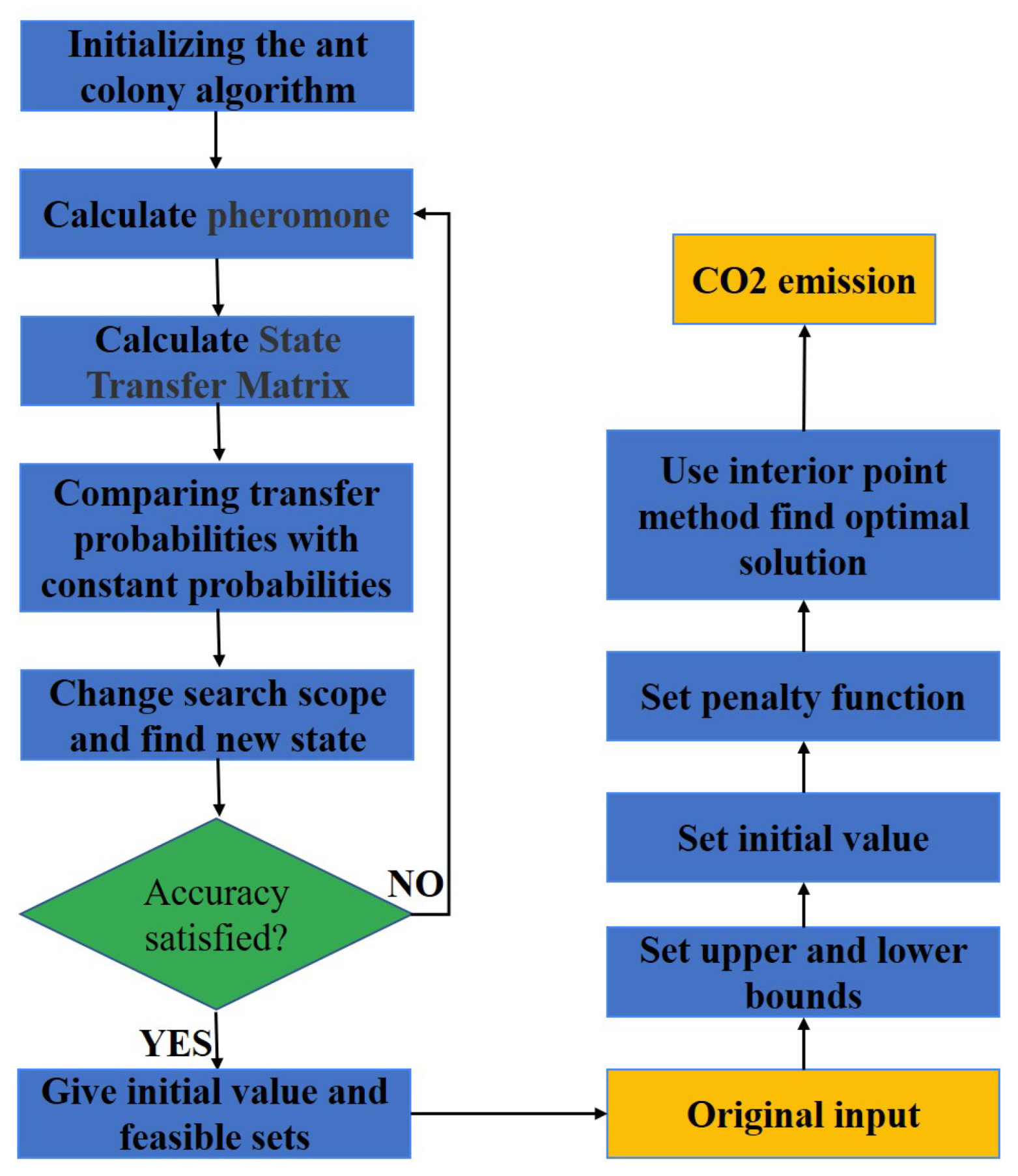
The ACA–IPFM model flow is shown in Figure 1.
3. Results
3.1. Simulation
In this study, we simulated the CO concentration measured by the mobile system based on Equation (1), which we set q, u, a, b, c, d, H, , B as Table 1 actual sets. However, in the actual measurement process, it is difficult to obtain the simulated measurement values under ideal conditions, so we added errors to the real values. We added 2% error to the measurement concentration, 0.2 m/s wind speed error, and 5 degree wind direction error. These errors conform to a normal distribution. On the basis of the above settings, we sampled every 10 m along the path at a vertical distance of 150 m from the emission source, using 70 sampling points as the measured values, and carried out the retrieval work. The retrieval results are shown in Table 1 and the vertical paths are shown in Figure 2.
As shown in Table 1, the optimal estimates are all very close to the true setting, where the CO emission error is only 0.51% and the uncertainty is only 1%.
3.2. Stability Analysis
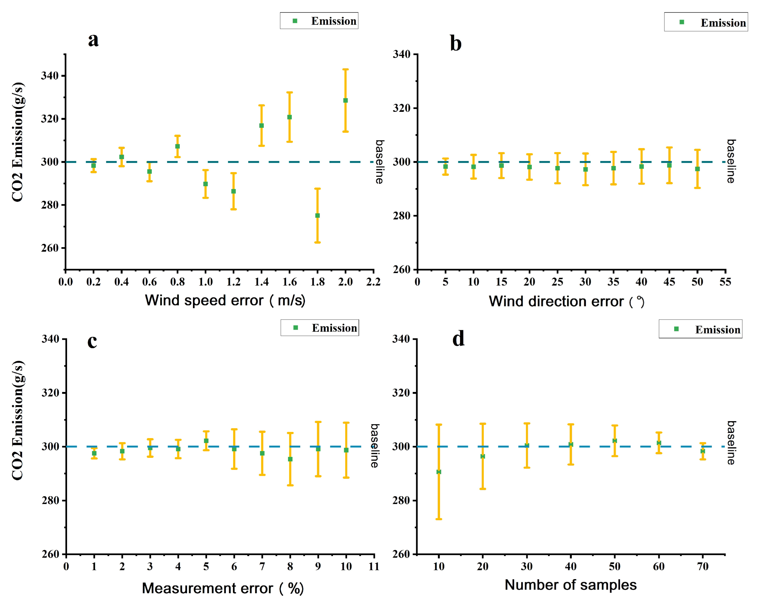
From Equation (1), we can find that wind speed error, wind direction error, measurement error, and sampling quantity all have negative effects on the final retrieval results, among which, although wind speed is directly measured by the mobile system, the error of the measurement value will be transferred to the final retrieval process, which eventually leads to the wrong estimation of CO emission q. For the wind direction error, although it cannot directly lead to the wrong estimation of CO emission q, the coordinates are established with the wind direction as the x-axis. The deviation of the wind direction estimation will in turn lead to the wrong estimation of the vertical and horizontal diffusion factors and transfer this error to the retrieval error. The measurement error, as the error carried by the instrument itself, directly affects the retrieval accuracy. It is certain that, as the measurement error increases, the uncertainty will increase. The number of samples directly affects the amount of information obtained, and more samples can better reduce the uncertainty of the retrieval. In order to evaluate the effectiveness of ACA–IPFM, as well as to quantitatively analyze the impact of the above error factors on the retrieval, we performed simulations for more cases as shown in Figure 3.
From Figure 3a, it can be found that the retrieval error value of CO emission increases gradually with the increase of wind speed error, but there is no obvious pattern for the retrieval error. There is, moreover, no obvious relationship between the overestimation or underestimation of CO emission and the increase of wind speed error. The retrieved uncertainty of CO emission is positively correlated with the increase of wind speed error, and the uncertainty increases with the increase of wind speed error. When the wind speed error is less than 0.8 m/s, the deviation of the optimal estimate of CO emissions is within 2.5%, and even at a wind speed error of 2 m/s, the optimal estimate of CO emissions can be controlled within 10%, which reflects the good robustness of the retrieval of ACA–IPFM within a certain wind speed error.
In Figure 3b, the wind direction error has less influence on the inversion of CO emissions than that brought by the wind speed error, and the optimal estimate of CO emissions is always near the true value with the maximum error within 1%, and there is a positive correlation between the uncertainty and the wind direction error. Although the wind direction error affects the establishment of the coordinate system, ACA–IPFM also has good robustness to the wind direction error because ACA–IPFM makes full use of the derivative information about the horizontal and vertical diffusion parameters in the Gaussian plume model.
In Figure 3c, we can see that the optimal estimate of CO emissions becomes more volatile as the measurement error increases, but the uncertainty is still controlled within 4% even when the measurement error is 10%, because the measurement error is always assumed to be Gaussian distributed, so minimizing can largely resist the effect of Gaussian noise.
From Figure 3d, it can be found that the volatility of the optimal estimate of CO emissions decreases as the number of samples increases. The deviation between the overall optimal estimate and the true value is always within 3.2%, and the uncertainty is always within 6%. This shows that, even in the small sampling range, ACA–IPFM still has good optimal estimation properties compared with the traditional least squares algorithm which has difficulty in accurately assessing CO emissions in the low sample case. We believe that this is due to the fact the ACA first searches for the approximate range of the global optimal solution, which leads to a more accurate retrieval performance of the interior point penalty function for CO emissions. However, the stability of ACA–IPFM is also limited by the number of samples: the more samples, the higher the stability. Therefore, we believe that ACA–IPFM has a great potential to accurately retrieve CO emissions when the number of samples is higher than 60.
3.3. Joint Error Analysis
In the actual measurement process, it is difficult for a single type of error to exist independently, and it is more likely that different types of errors of different sizes exist in combination.
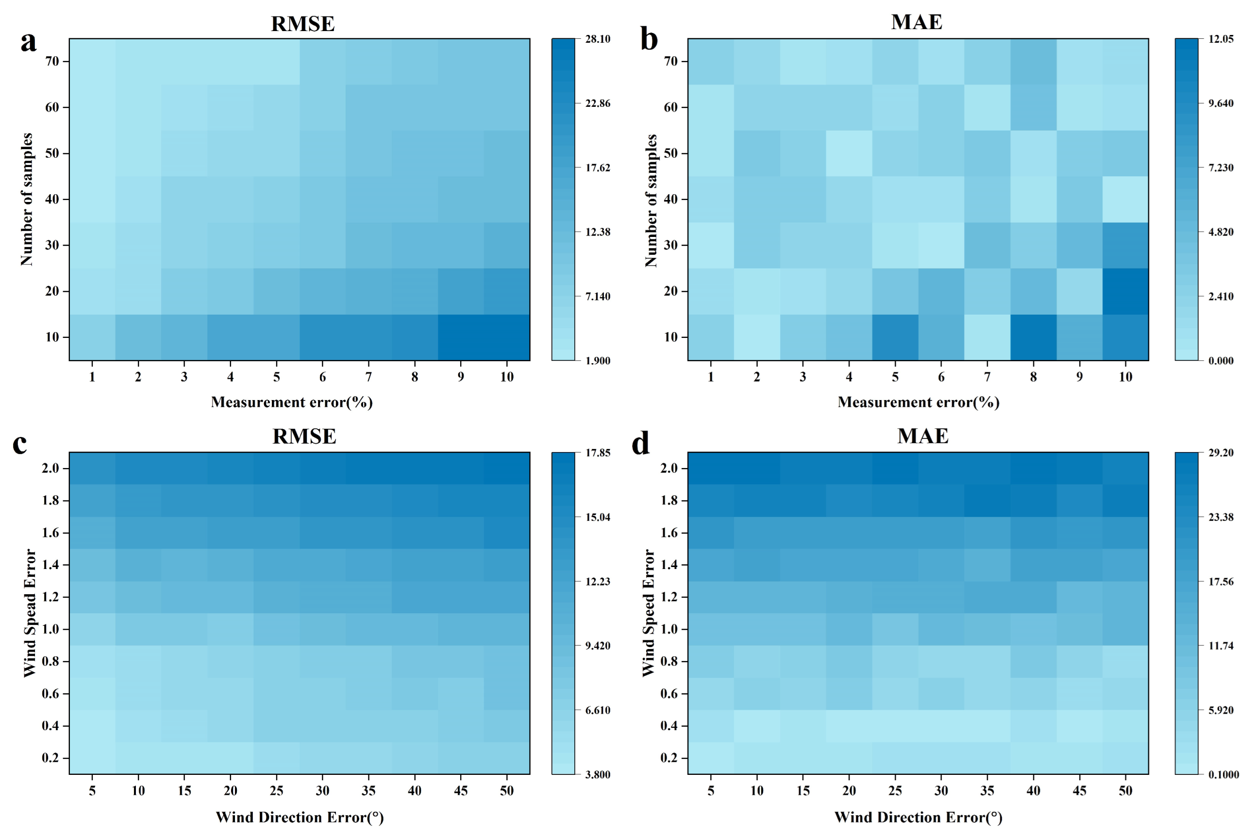
In order to better model the impact of multiple errors on the best estimate of CO emissions, we conducted a further analysis. In reality, wind speed and wind direction are a set of possible joint errors under the same observation conditions, when the number of CO concentration measurements and instrument measurement errors are stable, and when the wind speed and wind direction measurement errors are stable, different mobile instruments may differ in the number of measurements and measurement errors, and this joint error may also have a new impact on the CO emission inversion, and this assessment is also important. Therefore, in this section, we calculate the errors of CO emission retrieval for different combinations of wind speed error and wind direction error, and for different combinations of observation number and observation error. The results are shown in Figure 4.
In Figure 4a,b, it can be seen that the RMSE of the optimal estimate of CO emissions increases when the number of measurements is reduced and the measurement error increases. However, comparing the number of measurements with different concentrations, it can be found that the degree of influence of the measurement accuracy on the retrieval accuracy is different for different numbers of measurements. In the case of more measurements, the RMSE of the retrieved CO emissions with fewer measurements increases more sharply than that of the retrieved CO emissions with more measurements. As for the MAE of the optimal estimation of CO emissions, the MAE largely increases when the number of measurements decreases and the measurement error increases, but there will be a few cases where the MAE decreases, but the RMSE corresponding to this case is larger, so that its final corresponding error is still large. Therefore, when the measurement instrument error of the mobile measurement system is unstable, the impact of instrument measurement errors can be reduced by increasing the number of measurements. A similar pattern can be found in Figure 4c,d: with the increase of wind direction error and wind speed error, the RMSE of the optimal estimation of CO emission increases, and the MAE also increases largely with it, while the fluctuation of the optimal estimation caused by wind speed error is more drastic in the case of higher wind direction error. Therefore, in the actual measurement process, more accurate instruments should be used to minimize the degradation of CO emission retrieval accuracy caused by wind speed and wind direction errors.
3.4. Actual Experiment
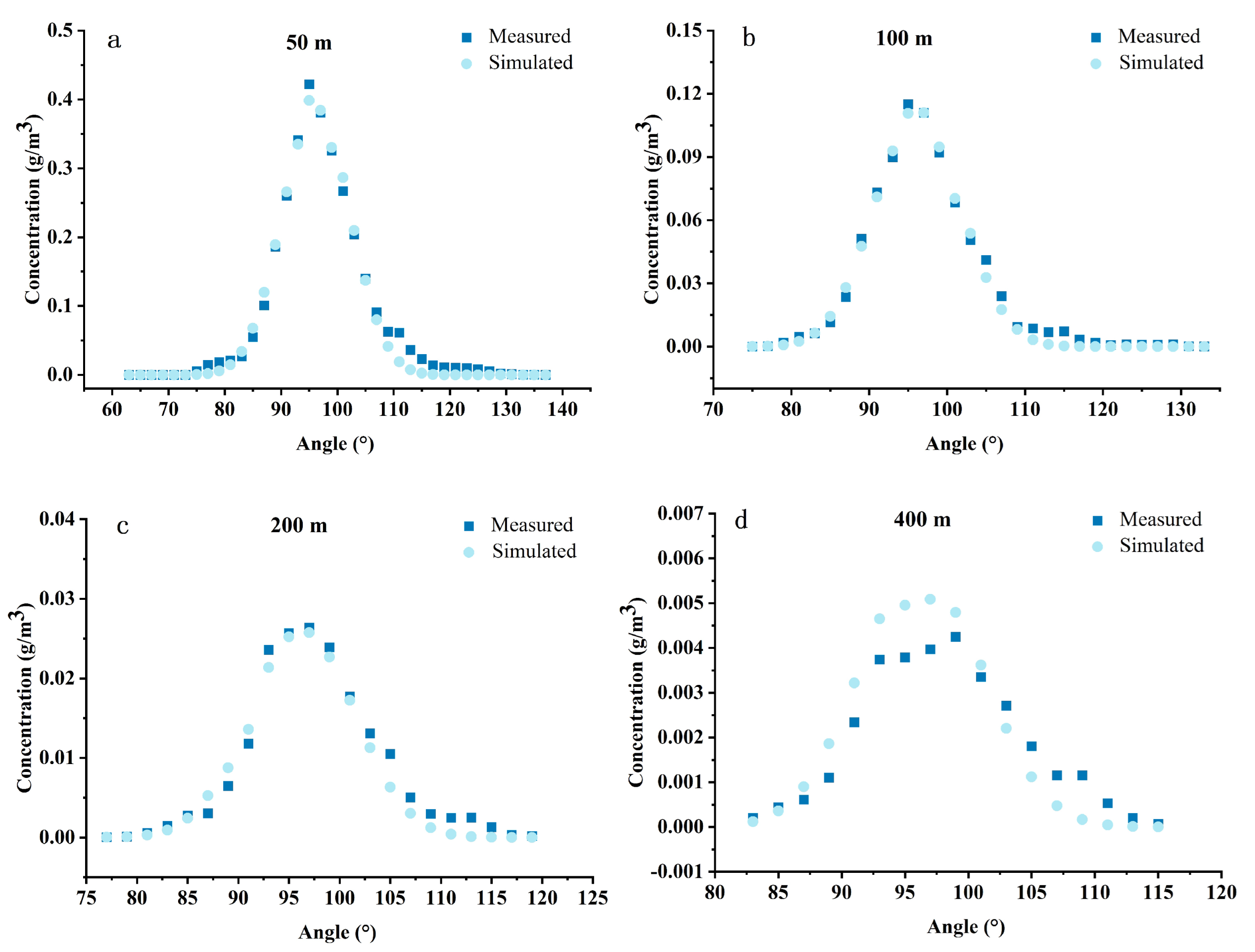
In this section, we retrieve the emissions though real data using the ACA–IPFM. Due to the lack of relevant real data for CO, we use the real data for SO instead. This dataset [27] was obtained from the Prairie Grass emission experiment and contains a total of five sets of measurements at 50 m, 100 m, 200 m, 400 m, and 800 m radius from the SO emission source. The wind speed was 4.85 ± 1 m/s and the wind direction was 184 ± 10° for the five sets of measurements. We discarded the measurements at 800 m because they contained too little useful information. Experiments were performed to retrieve SO emission on each set of observations, and we obtained the optimal estimates for each set. Based on the optimal estimates and the Gaussian plume model, the simulated SO concentrations at the corresponding measurement locations were simulated, and the results are shown in Figure 5.
The SO emission retrieved from ACA–IPFM is 90.7 g/s, while the real SO emission from this dataset is 91.1 g/s. The error between the two is only 0.43%. The difference between the simulated and real concentrations can be seen in Figure 5a–d. The difference in Figure 5d is more obvious, which may be due to the measurement distance being too far away from the SO emission source, leading a reduction in the SO concentration enhanced by emissions, and the measurement error of the instrument being amplified accordingly. These errors ultimately reduce the similarity between the simulated and real SO concentration values.
4. Discussion
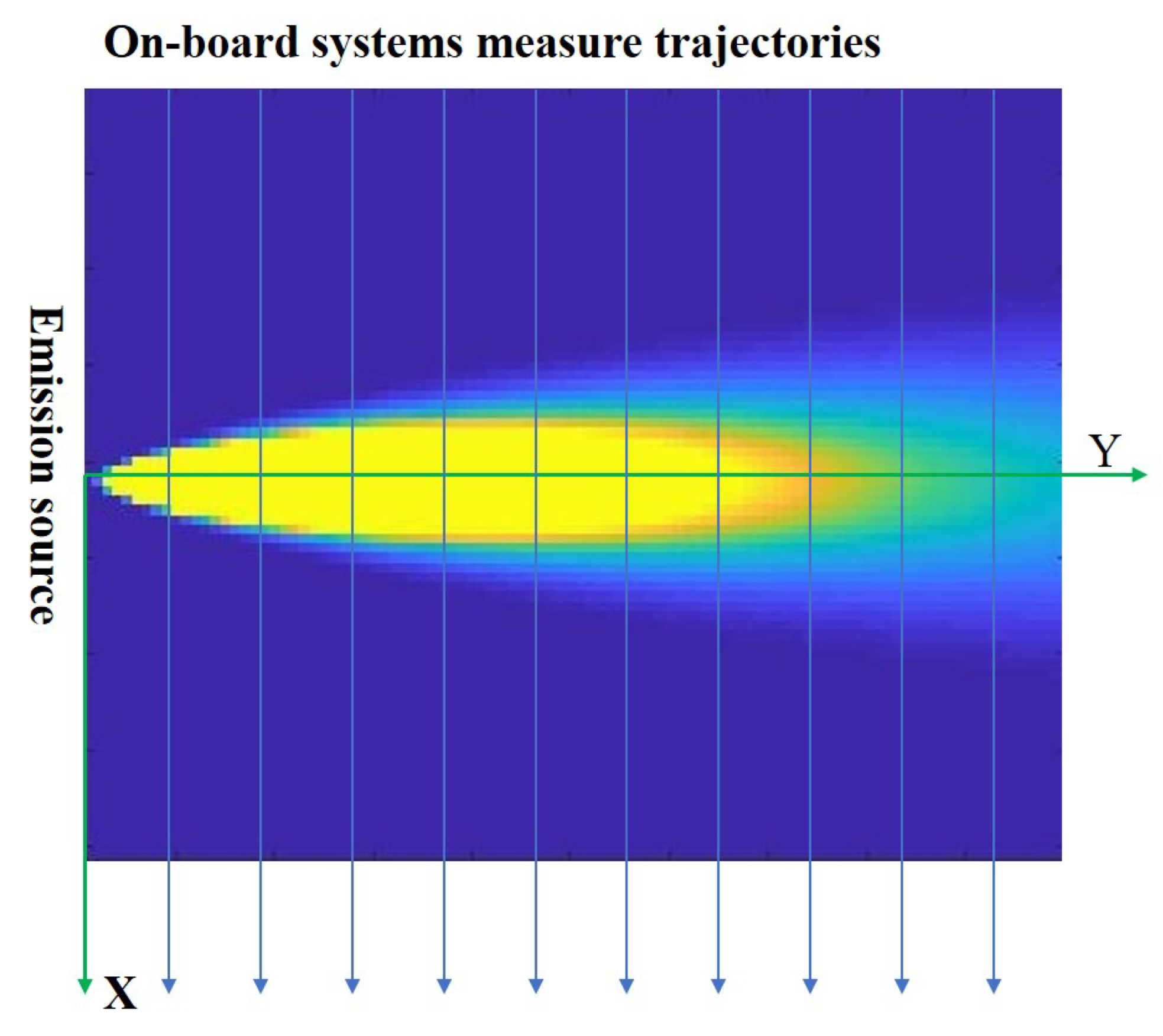
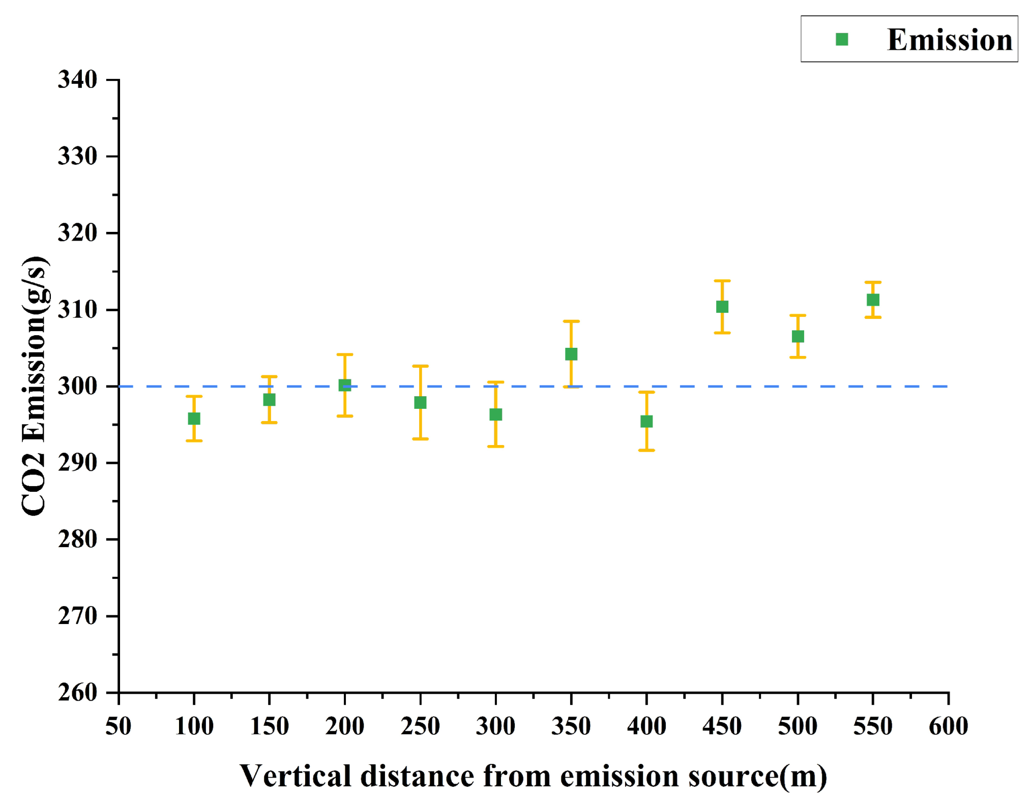
In actual measurements, we cannot always measure the CO concentration on the ideal path in the experiment due to the different observation conditions, topography conditions, and other factors. In Section 3, we have discussed various types of errors in detail, but these discussions are based on the case that the measurement path of the mobile system is 150 m from the vertical distance of the CO emission source. Obviously, in the actual measurement situation, it is difficult to guarantee that every observation path is this ideal case. Therefore, in this section, we further simulate the observations of the mobile system on different paths. These observations are simulated under the parameter settings of Table 1, and the simulated paths are from 100 m to 550 m vertical distance from the CO emission source with an interval of 50m, and the number of measurements is 70. The different measurement paths are shown in Figure 6. The simulated observations on different paths were used to retrieve the CO emissions and quantitatively evaluate the MAE and RMSE of the optimal estimates of CO emissions. The results are shown in Figure 7.
In Figure 7, as the vertical distance of the measurement path from the CO emission source increases, the RMSE of the optimal estimate of CO emission shows a trend of increasing and then decreasing, while the MAE shows a trend of aggregation to divergence. We believe this is due to the fact that observations on different pathways are affected differently by CO emissions. When the vertical distance is between 100 and 150 m, the measured values of CO concentration are dominated by the enhanced values of CO concentration, so the inverse CO emission has a better performance in both MAE and RMSE. When the vertical distance is between 200 m and 400 m, the measured values have some of the enhanced values of CO concentration in addition to the background values, of which the enhanced values are still the main component. The influence of this part of background values will make the MAE of the optimal estimation of CO emissions approach the true value but RMSE appear to increase; when the vertical distance is greater than 450 m, the MAE of the optimal estimation of CO emissions is far from the true value, but the RMSE will gradually decrease. It is due to the fact that, in this observation case, the CO concentration observation is gradually dominated by the background value, and the effect of the enhanced value gradually becomes weaker. Therefore, in the actual measurement process, when the vertical distance is between 200 m and 400 m, the number of measurements in the path should be increased so as to reduce the fluctuation of RMSE.
Benefiting from the flexibility of the mobile system itself and the accuracy of Gaussian plume model in simulating the gas transport, it is increasingly feasible to retrieve the CO emissions of emission sources by measuring CO concentration on the developed path with the mobile system. Through a series of simulations and error experiments, the feasibility and accuracy of ACA–IPFM for CO emission retrieval is further demonstrated, and the robustness of ACA–IPFM within a certain error range is verified from quantitative analysis. In the future, ACA–IPFM can provide a feasible solution for CO retrieval of mobile systems.
5. Conclusions
In this paper, we propose ACA–IPFM for retrieval of CO emissions from CO emission sources. This algorithm combines the property of global search of ACA and the nature of local exact search of the interior point penalty function to make the CO emission retrieval have better performance and robustness within a certain error range. The CO retrieval accuracy is evaluated in terms of different wind speed errors, wind direction errors, measurement errors and measurement numbers, and the effect of joint errors on the CO retrieval accuracy is also evaluated. The simulation experiments demonstrate that the optimal estimate of CO emissions is within 1% of MAE error and 3% of uncertainty when the remaining observation errors are within the normal range for the number of measurements greater than 60. Even when the wind speed error is within 30% of the original measurement value, the MAE error of the best estimate of CO emission is within 3% and the uncertainty is within 6%. ACA–IPFM can largely help the mobile system to achieve accurate CO emission retrieval, and combined with the agility of the mobile system itself, it will be promising to obtain more CO emission monitoring of CO emission sources in the region in the future.
Author Contributions
Investigation, H.M.; Methodology, M.C. and T.S.; Resources, M.C.; Supervision, H.M., C.C., X.W. and T.S.; Writing—original draft, M.C. All authors have read and agreed to the published version of the manuscript.
Funding
This work was supported by the National Natural Science Foundation of China (Grant No. 41971283 and No. 41601351).
Institutional Review Board Statement
Not applicable.
Informed Consent Statement
Informed consent was obtained from all subjects involved in the study.
Data Availability Statement
Not applicable.
Conflicts of Interest
The authors declare no conflict of interest.
References
- Oda, T.; Maksyutov, S. A very high-resolution (1 km × 1 km) global fossil fuel CO2 emission inventory derived using a point source database and satellite observations of nighttime lights. Atmos. Chem. Phys. 2011, 11, 543–556. [Google Scholar] [CrossRef]
- Friedlingstein, P.; Jones, M.W.; O’sullivan, M.; Andrew, R.M.; Hauck, J.; Peters, G.P.; Peters, W.; Pongratz, J.; Sitch, S.; Quéré, C.L.; et al. Global Carbon Budg. Earth Syst. Sci. Data 2019, 11, 1783–1838. [Google Scholar] [CrossRef]
- Liu, B.; Ma, X.; Ma, Y.; Li, H.; Jin, S.; Fan, R.; Gong, W. The relationship between atmospheric boundary layer and temperature inversion layer and their aerosol capture capabilities. Atmos. Res. 2022, 271, 106121. [Google Scholar] [CrossRef]
- Xu, W.; Wang, W.; Wang, N.; Chen, B. A new algorithm for himawari-8 aerosol optical depth retrieval by integrating regional PM2.5 concentrations. IEEE Trans. Geosci. Remote Sens. 2022, 60, 1–11. [Google Scholar] [CrossRef]
- Luo, B.; Yang, J.; Song, S.; Shi, S.; Gong, W.; Wang, A.; Du, L. Target classification of similar spatial characteristics in complex urban areas by using multispectral lidar. Remote Sens. 2022, 14, 238. [Google Scholar] [CrossRef]
- Zhang, J.; Han, G.; Mao, H.; Pei, Z.; Ma, X.; Jia, W.; Gong, W. The spatial and temporal distribution patterns of xch4 in china: New observations from tropomi. Atmosphere 2022, 13, 177. [Google Scholar] [CrossRef]
- Hu, Y.; Shi, Y. Estimating CO2 emissions from large scale coal-fired power plants using OCO-2 observations and emission inventories. Atmosphere 2021, 12, 811. [Google Scholar] [CrossRef]
- Bovensmann, H.; Buchwitz, M.; Burrows, J.; Reuter, M.; Krings, T.; Gerilowski, K.; Schneising, O.; Heymann, J.; Tretner, A.; Erzinger, J. A remote sensing technique for global monitoring of power plant CO2 emissions from space and related applications. Atmos. Meas. Tech. 2010, 3, 781–811. [Google Scholar] [CrossRef]
- Shindell, D.; Faluvegi, G. The net climate impact of coal-fired power plant emissions. Atmos. Chem. Phys. 2010, 10, 3247–3260. [Google Scholar] [CrossRef]
- Delre, A.; Mønster, J.; Scheutz, C. Greenhouse gas emission quantification from wastewater treatment plants, using a tracer gas dispersion method. Sci. Total Environ. 2017, 605, 258–268. [Google Scholar] [CrossRef]
- Shi, T.; Han, G.; Ma, X.; Gong, W.; Chen, W.; Liu, J.; Zhang, X.; Pei, Z.; Gou, H.; Bu, L. Quantifying CO2 uptakes over oceans using lidar: A tentative experiment in bohai bay. Geophys. Res. Lett. 2021, 48, e2020GL091160. [Google Scholar] [CrossRef]
- Zheng, B.; Chevallier, F.; Ciais, P.; Broquet, G.; Wang, Y.; Lian, J.; Zhao, Y. Observing carbon dioxide emissions over china’s cities and industrial areas with the orbiting carbon observatory-2. Atmos. Chem. Phys. 2020, 20, 8501–8510. [Google Scholar] [CrossRef]
- Klaaßen, L.; Stoll, C. Harmonizing corporate carbon footprints. Nat. Commun. 2021, 12, 1–13. [Google Scholar] [CrossRef]
- Liu, F.; Duncan, B.N.; Krotkov, N.A.; Lamsal, L.N.; Beirle, S.; Griffin, D.; McLinden, C.A.; Goldberg, D.L.; Lu, Z. A methodology to constrain carbon dioxide emissions from coal-fired power plants using satellite observations of co-emitted nitrogen dioxide. Atmos. Chem. Phys. 2020, 20, 99–116. [Google Scholar] [CrossRef]
- Gregg, J.S.; Andres, R.J.; Marland, G. China: Emissions pattern of the world leader in CO2 emissions from fossil fuel consumption and cement production. Geophys. Res. Lett. 2008, 35. [Google Scholar] [CrossRef]
- Shan, Y.; Liu, J.; Liu, Z.; Xu, X.; Shao, S.; Wang, P.; Guan, D. New provincial CO2 emission inventories in china based on apparent energy consumption data and updated emission factors. Appl. Energy 2016, 184, 742–750. [Google Scholar] [CrossRef]
- Wolff, S.; Ehret, G.; Kiemle, C.; Amediek, A.; Quatrevalet, M.; Wirth, M.; Fix, A. Determination of the emission rates of CO2 point sources with airborne lidar. Atmos. Meas. Technol. 2021, 14, 2717–2736. [Google Scholar] [CrossRef]
- Nassar, R.; Hill, T.G.; McLinden, C.A.; Wunch, D.; Jones, D.B.; Crisp, D. Quantifying CO2 emissions from individual power plants from space. Geophys. Res. Lett. 2017, 44, 10–45. [Google Scholar] [CrossRef]
- Burrows, J.; Hölzle, E.; Goede, A.; Visser, H.; Fricke, W. Sciamachy—Scanning imaging absorption spectrometer for atmospheric chartography. Acta Astronaut. 1995, 35, 45–451. [Google Scholar] [CrossRef]
- Kuze, A.; Suto, H.; Nakajima, M.; Hamazaki, T. Thermal and near infrared sensor for carbon observation fourier-transform spectrometer on the greenhouse gases observing satellite for greenhouse gases monitoring. Appl. Opt. 2009, 48, 6716–6733. [Google Scholar] [CrossRef]
- O’Dell, C.; Connor, B.; Bösch, H.; O’Brien, D.; Frankenberg, C.; Castano, R.; Christi, M.; Eldering, D.; Fisher, B.; Gunson, M.; et al. The Acos CO2 retrieval Algorithm-1: Description and validation against synthetic observations. Atmos. Meas. Technol. 2012, 5, 99–121. [Google Scholar] [CrossRef]
- Pei, Z.; Han, G.; Ma, X.; Shi, T.; Gong, W. A method for estimating the background column concentration of CO2 using the lagrangian approach. IEEE Trans. Geosci. Remote Sens. 2022, 60, 4108112. [Google Scholar] [CrossRef]
- Chevallier, F.; Maksyutov, S.; Bousquet, P.; Bréon, F.-M.; Saito, R.; Yoshida, Y.; Yokota, T. On the accuracy of the CO2 surface fluxes to be estimated from the gosat observations. Geophys. Res. Lett. 2009, 36. [Google Scholar] [CrossRef]
- Han, G.; Cui, X.; Liang, A.; Ma, X.; Zhang, T.; Gong, W. A co 2 profile retrieving method based on chebyshev fitting for ground-based dial. IEEE Trans. Geosci. Remote Sens. 2017, 55, 6099–6110. [Google Scholar] [CrossRef]
- Nassar, R.; Mastrogiacomo, J.-P.; Bateman-Hemphill, W.; McCracken, C.; MacDonald, C.G.; Hill, T.; O’Dell, C.W.; Kiel, M.; Crisp, D. Advances in quantifying power plant CO2 emissions with OCO-2. Remote Sens. Environ. 2021, 264, 112579. [Google Scholar] [CrossRef]
- Wang, S.; Zhang, Q.; Martin, R.V.; Philip, S.; Liu, F.; Li, M.; Jiang, X.; He, K. Satellite measurements oversee china’s sulfur dioxide emission reductions from coal-fired power plants. Environ. Res. Lett. 2015, 10, 114015. [Google Scholar] [CrossRef]
- Ma, D.; Zhang, Z. Contaminant dispersion prediction and source estimation with integrated gaussian-machine learning network model for point source emission in atmosphere. J. Hazard. Mater. 2016, 311, 237–245. [Google Scholar] [CrossRef] [PubMed]
- Shi, T.; Han, G.; Ma, X.; Zhang, M.; Pei, Z.; Xu, H.; Qiu, R.; Zhang, H.; Gong, W. An inversion method for estimating strong point carbon dioxide emissions using a differential absorption lidar. J. Clean. Prod. 2020, 271, 122434. [Google Scholar] [CrossRef]
- Andersen, T.; Vinkovic, K.; de Vries, M.; Kers, B.; Necki, J.; Swolkien, J.; Roiger, A.; Peters, W.; Chen, H. Quantifying methane emissions from coal mining ventilation shafts using an unmanned aerial vehicle (uav)-based active aircore system. Atmos. Environ. X 2021, 12, 100135. [Google Scholar] [CrossRef]
- Han, G.; Gong, W.; Lin, H.; Ma, X.; Xiang, Z. Study on influences of atmospheric factors on vertical profile retrieving from ground-based dial at 1.6 μm. IEEE Trans. Geosci. Remote Sens. 2014, 53, 3221–3234. [Google Scholar] [CrossRef]
- Han, G.; Ma, X.; Liang, A.; Zhang, T.; Zhao, Y.; Zhang, M.; Gong, W. Performance evaluation for china’s planned CO2-ipda. Remote Sens. 2017, 9, 768. [Google Scholar] [CrossRef]
- Ehret, G.; Kiemle, C.; Wirth, M.; Amediek, A.; Fix, A.; Houweling, S. Space-borne remote sensing of CO2, CH4, and N2O by integrated path differential absorption lidar: A sensitivity analysis. Appl. Phys. B 2008, 90, 593–608. [Google Scholar] [CrossRef]
- Ehret, G.; Bousquet, P.; Pierangelo, C.; Alpers, M.; Millet, B.; Abshire, J.B.; Bovensmann, H.; Burrows, J.P.; Chevallier, F.; Ciais, P.; et al. Ger. Space Lidar Mission Dedic. Atmos. Remote Sens. 2017, 9, 1052. [Google Scholar] [CrossRef]
- Shi, T.; Han, G.; Ma, X.; Gong, W.; Pei, Z.; Xu, H.; Qiu, R.; Zhang, H.; Zhang, J. Potential of ground-based multiwavelength differential absorption lidar to measure δ13c in open detected path. IEEE Geosci. Remote Sens. Lett. 2021, 19, 1–4. [Google Scholar] [CrossRef]
- Xiang, C.; Ma, X.; Zhang, X.; Han, G.; Zhang, W.; Chen, B.; Liang, A.; Gong, W. Design of inversion procedure for the airborne co 2-ipda lidar: A preliminary study. IEEE J. Sel. Top. Appl. Earth Obs. Remote Sens. 2021, 14, 11840–11852. [Google Scholar] [CrossRef]
- Krings, T.; Gerilowski, K.; Buchwitz, M.; Reuter, M.; Tretner, A.; Erzinger, J.; Heinze, D.; Pflüger, U.; Burrows, J.; Bovensmann, H. Mamap–a new spectrometer system for column-averaged methane and carbon dioxide observations from aircraft: Retrieval algorithm and first inversions for point source emission rates. Atmos. Meas. Technol. 2011, 4, 1735–1758. [Google Scholar] [CrossRef]
- Shi, T.; Han, Z.; Gong, W.; Ma, X.; Han, G. High-precision methodology for quantifying gas point source emission. J. Clean. Prod. 2021, 320, 128672. [Google Scholar] [CrossRef]
- Pei, Z.; Han, G.; Ma, X.; Su, H.; Gong, W. Response of major air pollutants to covid-19 lockdowns in china. Sci. Total Environ. 2020, 743, 140879. [Google Scholar] [CrossRef]
- Arystanbekova, N.K. Application of gaussian plume models for air pollution simulation at instantaneous emissions. Math. Comput. Simul. 2004, 67, 451–458. [Google Scholar] [CrossRef]
- Miller, C.; Hively, L. A review of validation studies for the gaussian plume atmospheric dispersion model. Nucl. Saf. 1987, 28, 5588029. [Google Scholar]
- Dorigo, M.; Birattari, M.; Stutzle, T. Ant colony optimization. IEEE Comput. Intell. Mag. 2006, 1, 28–39. [Google Scholar] [CrossRef]
- Dorigo, M.; Stützle, T. Ant colony optimization: Overview and recent advances. In Handbook of Metaheuristics; Springer: Berlin/Heidelberg, Germany, 2019; pp. 311–351. [Google Scholar] [CrossRef]
- Yeniay, Ö. Penalty function methods for constrained optimization with genetic algorithms. Math. Comput. Appl. 2005, 10, 45–56. [Google Scholar] [CrossRef]
- Levenberg, K. A method for the solution of certain non-linear problems in least squares. Q. Appl. Math. 1944, 2, 164–168. [Google Scholar] [CrossRef]
- Marquardt, D.W. An algorithm for least-squares estimation of nonlinear parameters. J. Soc. Ind. Appl. Math. 1963, 11, 431–441. [Google Scholar] [CrossRef]
Figure 1.
Flow chart of ACA–IPFM model.

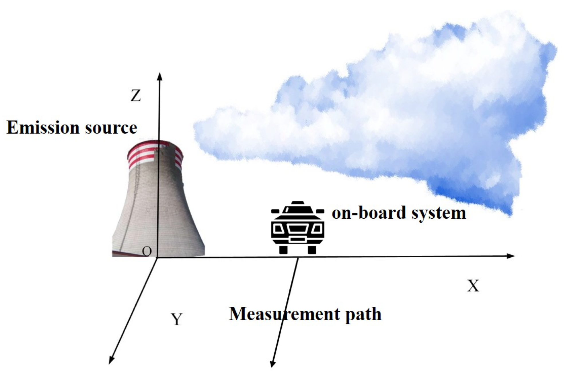
Figure 2.
Mobile system measurement schematic.

Figure 3.
Effect of four types of errors on retrieval results. The base set is the same as Table 1 and the baseline is the actual CO emission; (a) add additional errors to wind speed from 0.2 m/s to 2.0 m/s with internal of 0.2 m/s; (b) add errors for wind direction, increase the range from 5 degrees to 50 degrees with an interval of 5 degrees; (c) adding random error for the measurement, from 1% measurement error increase to 10% error with an interval of 1%; (d) changing the number of samples from 10 to 70 with an interval of 10.

Figure 4.
Effect of joint error on retrieval accuracy. (a,b) RMSE and MAE for optimal estimation of CO emissions under the combined effect of measurement error and measurement number, respectively, with measurement error from 1% to 10% and measurement number from 10 to 70. (c,d) RMSE and MAE for optimal estimation of CO emissions under the combined effect of wind direction error and wind speed error, respectively, with wind direction error from 5 degrees to 50 degrees and wind speed error from 0.2 m/s to 2 m/s.

Figure 5.
Simulated SO concentrations through Gaussian plume model based on the parameters calculated by ACA–IPFM. Angle is the angle from the west direction, (a) is the measurements at 50 m radius of the SO emission source, (b) is the measurements at 100 m radius of the SO emission source, (c) is the measurements at 200 m radius of the SO emission source, (d) is the measurements at 800 m radius of the SO emission source.

Figure 6.
Schematic diagram of the different measurement trajectories of the mobile system.

Figure 7.
CO emission retrieval results under different measurement paths.


Table 1.
Parameters of Gaussian plume model and the retrieval results.
| Parameters | Actual Sets | Retrieval Results |
|---|---|---|
| CO Emission q (g/s) | 300 | 298.29 ± 3.01 |
| Wind speed u (m/s) | 3 | 3 ± 0.02 |
| a | 0.11 | 0.13 ± 0.02 |
| b | 0.92 | 0.90 ± 0.05 |
| c | 0.11 | 0.12 ± 0.04 |
| d | 0.83 | 0.80 ± 0.02 |
| H | 10 | 10.2 ± 0.02 |
| 0.95 | 0.93 ± 0.05 | |
| B | 1500 | 1503 ± 2.5 |
| Wind direction | 90 | 90.2 ± 0.3 |
Publisher’s Note: MDPI stays neutral with regard to jurisdictional claims in published maps and institutional affiliations. |
© 2022 by the authors. Licensee MDPI, Basel, Switzerland. This article is an open access article distributed under the terms and conditions of the Creative Commons Attribution (CC BY) license (https://creativecommons.org/licenses/by/4.0/).
Share and Cite
MDPI and ACS Style
Cai, M.; Mao, H.; Chen, C.; Wei, X.; Shi, T. Measuring Greenhouse Gas Emissions from Point Sources with Mobile Systems. Atmosphere 2022, 13, 1249. https://0-doi-org.brum.beds.ac.uk/10.3390/atmos13081249
AMA Style
Cai M, Mao H, Chen C, Wei X, Shi T. Measuring Greenhouse Gas Emissions from Point Sources with Mobile Systems. Atmosphere. 2022; 13(8):1249. https://0-doi-org.brum.beds.ac.uk/10.3390/atmos13081249
Chicago/Turabian StyleCai, Mengyang, Huiqin Mao, Cuihong Chen, Xvpeng Wei, and Tianqi Shi. 2022. "Measuring Greenhouse Gas Emissions from Point Sources with Mobile Systems" Atmosphere 13, no. 8: 1249. https://0-doi-org.brum.beds.ac.uk/10.3390/atmos13081249
Note that from the first issue of 2016, this journal uses article numbers instead of page numbers. See further details here.