
Observation and Simulation of CO2 Fluxes in Rice Paddy Ecosystems Based on the Eddy Covariance Technique

1
School of Resources and Environmental Engineering, Jiangsu University of Technology, Changzhou 213001, China
2
Department of Environmental Science and Engineering, Fudan University, Shanghai 200438, China
3
Collaborative Innovation Center of Atmospheric Environment and Equipment Technology, Jiangsu Key Laboratory of Atmospheric Environment Monitoring and Pollution Control (AEMPC), Nanjing University of Information Science & Technology, Nanjing 210044, China
*
Author to whom correspondence should be addressed.
Atmosphere 2024, 15(5), 517; https://0-doi-org.brum.beds.ac.uk/10.3390/atmos15050517
Submission received: 2 April 2024
/
Revised: 21 April 2024
/
Accepted: 23 April 2024
/
Published: 24 April 2024
(This article belongs to the Special Issue Ozone Pollution and Effects in China)
Abstract
:As constituents of one of the vital agricultural ecosystems, paddy fields exert significant influence on the global carbon cycle. Therefore, conducting observations and simulations of CO2 flux in rice paddy is of significant importance for gaining deeper insights into the functionality of agricultural ecosystems. This study utilized an eddy covariance system to observe and analyze the CO2 flux in a rice paddy field in Eastern China and also introduced and parameterized the Jarvis multiplicative model to predict the CO2 flux. Results indicate that throughout the observation period, the range of CO2 flux in the paddy field was −0.1 to −38.4 μmol/(m2·s), with a mean of −12.9 μmol/(m2·s). The highest CO2 flux occurred during the rice flowering period with peak photosynthetic activity and maximum CO2 absorption. Diurnal variation in CO2 flux exhibited a “U”-shaped curve, with flux reaching its peak absorption at 11:30. The CO2 flux was notably higher in the morning than in the afternoon. The nocturnal CO2 flux remained relatively stable, primarily originating from respiratory CO2 emissions. The rice canopy CO2 flux model was revised using boundary line analysis, elucidating that photosynthetically active radiation, temperature, vapor pressure deficit, phenological stage, time, and concentration are pivotal factors influencing CO2 flux. The simulation of CO2 flux using the parameterized model, compared with measured values, reveals the efficacy of the established parameter model in simulating rice CO2 flux. This study holds significant importance in comprehending the carbon cycling process within paddy ecosystems, furnishing scientific grounds for future climate change and environmental management endeavors.
1. Introduction
The Intergovernmental Panel on Climate Change (IPCC) Fifth Assessment Report unequivocally states that global climate warming is an indisputable fact. The primary cause of global warming is the continuous increase in the emissions of greenhouse gases such as carbon dioxide (CO2), methane (CH4), nitrous oxide (N2O), and water vapor in the atmosphere. This leads to an excessive absorption of solar radiation and other energy reflected from the Earth’s surface by the atmosphere, resulting in the greenhouse effect and ultimately causing gradual global warming [1]. Since the Industrial Revolution, with the development of social productivity and the expansion of economic scale, human emissions of greenhouse gases, primarily CO2, have increased sharply. Currently, excessive CO2 emissions are considered the primary cause of anthropogenic influence on the greenhouse effect. Studies have shown that the global atmospheric CO2 concentration has risen from 315 ppm in the mid-20th century to the current 368 ppm, with emissions from fossil fuel combustion accounting for 57% of total greenhouse gas emissions [2].
Constituting one of the four major carbon reservoirs globally, terrestrial ecosystems serve as a bridge for CO2 exchange between the atmosphere and the biosphere. They not only utilize vegetation photosynthesis to absorb and store CO2 from the atmosphere, acting as carbon sinks, but also release CO2 into the atmosphere through vegetation and soil respiration, serving as stable carbon sources [3]. It is this unique dual nature of terrestrial ecosystems that gives them a pivotal role in the global carbon balance. Terrestrial ecosystems are primarily composed of forest ecosystems, grassland ecosystems, and agricultural ecosystems. Compared to the other two land covers, agricultural ecosystems are more susceptible to human production activities, thus exhibiting more variability in CO2 exchange and warranting further research [4]. Furthermore, research on CO2 fluxes both domestically and internationally has predominantly focused on forests and grasslands, leaving relatively little attention to agricultural ecosystems [5]. Therefore, studying the carbon fluxes in agricultural ecosystems is of significant importance for a deeper understanding of the carbon cycling patterns within terrestrial ecosystems and for predicting future global changes.
Currently, there are mainly two methods for observing CO2 flux: the chamber method and micrometeorological methods [6]. Among them, the chamber method, due to its simplicity and low cost, has been widely used, and most domestic studies are based on this method [7]. When using this method for measurement, the chamber needs to be closed, which changes the growth environment of the crop to some extent, thus affecting the accuracy of the experimental results [7]. The gradient method and the eddy covariance method are two commonly used micrometeorological methods for observing CO2 flux in ecosystems. When using the gradient method to measure atmospheric CO2 flux, observations of CO2 concentration, wind speed, temperature, humidity, etc. need to be made at different heights above the crop canopy to calculate CO2 flux [8]. This method requires high requirements for gas analyzers and sampling systems and suitable meteorological conditions during observations [8,9]. The micrometeorological method based on the eddy covariance technique is an advanced method developed in recent years for measuring atmospheric fluxes in ecosystems. This method is still relatively scarce in the observation of CO2 and water vapor fluxes; thus, further research is necessary [10]. On the other hand, previous studies on CO2 flux have mainly focused on field observations. Given the complex factors affecting CO2 flux and the limited efficacy of single-factor analysis, it is necessary to integrate multiple influencing factors and establish suitable models for predicting CO2 flux.
Based on the concerns mentioned above, the present study employed an eddy covariance system to continuously observe the CO2 flux within the rice canopy and analyze its variation characteristics. Furthermore, the study introduced and parameterized a canopy CO2 flux model to predict CO2 flux, thereby providing important foundations for the accurate assessment of ecosystem carbon fluxes in China and the formulation of strategies for sustainable agricultural development. This research aims to offer scientific support for the formulation of relevant policies and the sustainable development of agricultural production.
2. Materials and Methods
2.1. Site Description
The observation site is located in the rice paddies of the Yongfeng Agricultural Meteorological Station at Nanjing University of Information Science and Technology (32°21′ N, 118°69′ E, elevation: approximately 22 m). The observation period for CO2 flux in the rice paddies was from 15 July 2017 to 8 October 2017. The site covers an area that is approximately 250 m in length and 150 m in width, with an open and flat terrain and no tall buildings obstructing the surrounding area [11]. The soil type at the site is primarily yellow–brown soil, with a pH value of approximately 7.0. The soil organic matter content is 12.8 g·kg−1, total nitrogen content is 0.82 g·kg−1, available phosphorus content is 4.4 mg·kg−1, and available potassium content is 52.1 g·kg−1.
2.2. Observation Instruments
The CO2 flux observation instrument used in this study is an open-path eddy covariance system. Based on the eddy covariance principle, it utilizes fast-response sensors to measure the exchange of substances and energy between the atmosphere and the underlying surface. This method is considered the best approach for measuring carbon and water exchange fluxes in terrestrial ecosystems in recent years and has become the main technology of international flux observation networks. The eddy covariance system mainly consists of a CSAT3 three-dimensional sonic anemometer (Campbell Scientific Inc., Logan, UT, USA) and an LI-7500 H2O/CO2 infrared gas analyzer (LI-COR Biosciences, Lincoln, NE, USA), used to observe three-dimensional wind speed, sonic temperature, CO2, water vapor concentration, etc. The original data are sampled at a frequency of 10 Hz and recorded and processed online by the CR3000 data logger, and 30 min flux values and other parameters are stored in the data logger.
It should be noted that the CO2 uptake fluxes discussed in this study represent the daytime net ecosystem carbon exchange (NEE), namely the net CO2 uptake by rice, denoted as follows:
Here, Fc represents the CO2 turbulent flux, which can be directly obtained through the eddy covariance system; Fst represents the atmospheric CO2 storage flux below the instrument height; h is the height of the eddy covariance system; and ∆c represents the change in CO2 concentration over the time interval ∆t.
2.3. Data Processing
The raw data obtained through the eddy covariance system have a sampling frequency of 10 Hz. The 30 min flux calculations and preprocessing were performed using the EddyPro (v6.2.2, LI-COR Inc., Lincoln, NE, USA) software. This software is highly versatile and has been widely used for calculating fluxes of CO2, H2O, CH4, and other trace gases and energy. The preprocessing steps include outlier removal, time delay correction, secondary coordinate axis rotation, frequency response correction, and water vapor density correction among others [12]. To ensure data accuracy, the 30 min flux data outputted by the software require further quality control, as described below.
Firstly, data with negative values occurring during nighttime (when total solar radiation < 10 W·m−2) are removed. Secondly, outlier data that significantly deviate from the normal range of data variation are eliminated. Since precipitation can disrupt the normal atmospheric flow in agricultural ecosystems and may even lead to instrument malfunction, data collected during rainy periods are also excluded [11]. Finally, flux data corresponding to friction wind speeds less than 0.15 m·s−1 are removed to eliminate the influence of insufficiently developed turbulence [12].
Throughout the entire observation period, adverse weather conditions, instrument failures, power outages, and other factors may lead to a significant number of missing data. Therefore, it is necessary to interpolate the missing data mentioned above. The interpolation methods mainly include the following: for <3 h of continuous missing data, simple linear interpolation is applied [9]; for >3 h and <1 day of continuous missing data, the daily average change method is used [13]. In addition, continuous missing data lasting >1 day are not interpolated and are considered invalid data.
2.4. CO2 Flux Model
Based on the study by Tong et al. [14], the Jarvis stomatal conductance multiplicative model for rice leaves is extended to simulate the CO2 flux within the rice canopy. The specific expression of this model is as follows:
Here, represents the CO2 absorption flux of rice and is the maximum CO2 absorption flux. fmin is the ratio of minimum CO2 flux to maximum CO2 flux. ftemp, fVPD, fPAR, fphen, fTime, and represent the stress coefficients of temperature (T), vapor pressure deficit (VPD), photosynthetically active radiation (PAR), phenology (Phen), time (Time), and CO2 concentration to the maximum canopy CO2 flux, respectively [14]. These values are all within the range of 0 to 1. The parameters of each stress coefficient are obtained through the boundary line analysis technique of quantile regression [15]. Specifically, scatter plots are made with each climatic environmental variable as the horizontal axis and relative canopy CO2 flux as the vertical axis. Using the form of stress coefficients provided in the literature, the peripheral data points are fitted, thus obtaining the specific expressions of stress coefficients suitable for the rice CO2 flux model in the local area.
- (1)
- Temperature stress coefficient (ftemp)
- (2)
- Vapor pressure deficit stress coefficient (fVPD)
- (3)
- Photosynthetically active radiation stress coefficient (fPAR)
- (4)
- Phenology stress coefficient (fphen)
- (5)
- Time stress coefficient (fTime)
- (6)
- CO2 concentration stress coefficient (fCO2)
3. Results and Discussion
3.1. Variations in Meteorological Factors and CO2 Concentration
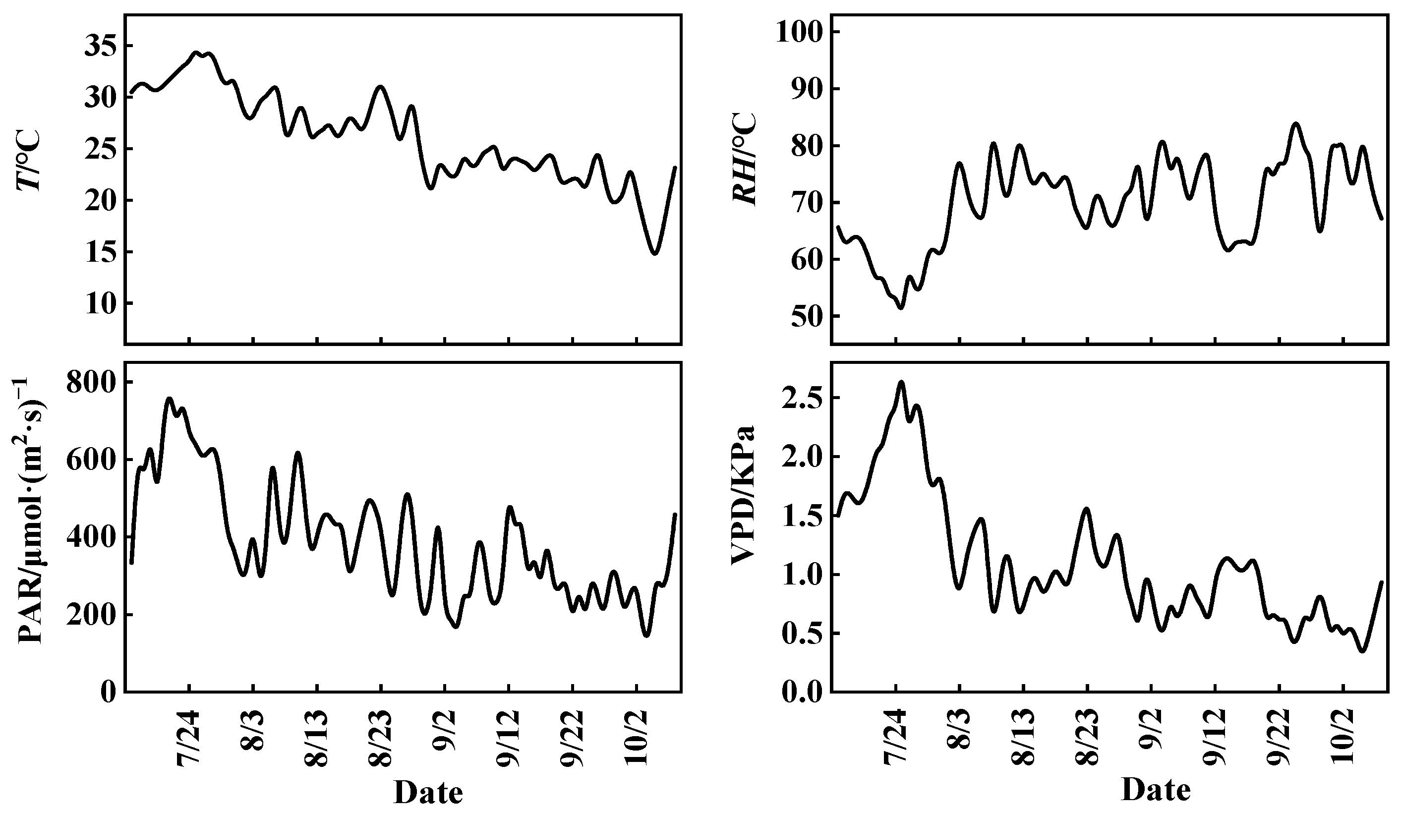
Figure 1 illustrates the daily variations in meteorological factors such as T, relative humidity (RH), PAR, and VPD during the rice growing season. It can be observed that the daily average ranges of T, RH, PAR, and VPD during the rice growing season are 14.1~34.7 °C, 49.1~84.8%, 128~786 μmol·(m2·s)−1, and 0.25~2.81 KPa, respectively, with means of 26.1 °C, 69.9%, 387.9 μmol·(m2·s)−1, and 1.10 KPa.
Figure 2 illustrates the diurnal variations in CO2 concentration during the rice growing season. The overall pattern of CO2 concentration shows a distinct “peak-trough” pattern, with lower levels during the day and higher levels at night, similar to the observations of previous studies [16]. From sunrise, as atmospheric turbulence and rice photosynthetic activity intensify, the CO2 concentration in the atmosphere begins to decrease rapidly, reaching its minimum around 16:00. This is attributed to the unstable boundary layer in the afternoon, which enhances turbulent exchange, facilitating the diffusion of CO2. Meanwhile, the strong photosynthetic activity of rice in the afternoon absorbs a considerable amount of CO2 [17]. Subsequently, due to the weakening of rice photosynthesis and convective transport (i.e., reduced CO2 sink strength), CO2 released from soil and biological respiration, industrial production, etc., gradually accumulates in the atmosphere, leading to an upward trend in concentration until it peaks the following morning.
3.2. The Variation in CO2 Flux
Figure 3 shows the time series variation in 30 min averaged CO2 flux during daytime periods throughout the rice growing season. Due to factors such as instrument malfunctions, power outages at the site, and weather conditions, data are missing for the following dates: 24–25 July, 30–31 July, 4–8 August, 10 August, 12 August, 14 August, 3–4 September, 24–25 September, 30 September, 2 October, and 5 October. Data for all other times remain intact. It is important to note that the 30 min CO2 flux data observed by the eddy covariance system represent the net carbon exchange (NEE) between the terrestrial ecosystem and the atmosphere. Therefore, the CO2 flux described in this study represented the NEE, indicating the net CO2 uptake by rice, with negative values indicating downward flux. As shown in the Figure 3, the range of 30 min CO2 flux throughout the entire rice observation period varies from −0.1 to −38.4 μmol·(m2·s)−1, with an average of −12.9 μmol·(m2·s)−1. Combining these results with Figure 4, it can be seen that the CO2 flux reaches its highest value during the flowering stage of rice. This might be attributed to the peak physiological activity of rice during this stage, characterized by vigorous photosynthesis and greater canopy conductance, resulting in enhanced CO2 uptake by the rice [18]. Although CO2 concentration remains relatively high during the later stages of the growing season, the reduced physiological activity of rice at this time leads to a slowdown in CO2 uptake.
Since the observed CO2 flux reflects the exchange of CO2 between the soil, vegetation, and the atmosphere, namely the remainder after deducting the total ecosystem respiration (Reco) from the gross primary productivity (GPP), the magnitude of CO2 flux indicates the intensity of this condition. If the intensity of photosynthesis of crop exceeds that of soil/crop respiration, the crop’s CO2 uptake is represented as net absorption, with a negative flux. Conversely, soil/crop releases CO2 to the atmosphere, with a positive flux.
The diurnal variation in CO2 flux during the rice growing season indicates a U-shaped curve (Figure 5). The nighttime CO2 flux is positive and relatively stable, indicating that the rice field ecosystem is a source of atmospheric CO2. The daytime CO2 flux is negative, indicating that CO2 uptake is predominant in the rice ecosystem. The flux value of rice changes from positive to negative between 06:30 and 07:00, indicating a transition of the ecosystem from a carbon source to a carbon sink. Subsequently, with the increase in solar radiation intensity, CO2 flux rapidly increases and reaches its maximum around 11:30, followed by a slow decrease until 12:00, when an abnormal decrease occurs. This is the phenomenon of “midday depression”, which occurs due to intense sunlight and disappears as sunlight diminishes, consistent with earlier observations at the same location [19]. The occurrence of this phenomenon is related to “photoinhibition” occurring after photosynthetically active radiation reaches the light saturation point. This can be explained as follows: CO2/H2O flux and canopy conductance increase with the enhancement of photosynthetically active radiation starting from the morning. When the light saturation point of crop leaves is reached, “photoinhibition” occurs, resulting in a decrease in CO2 absorption flux. Crops respond to strong light by exhibiting physiological reactions such as upper leaf curling and reduction in effective leaf area, leading to a decrease in water vapor flux and canopy conductance [20]. As photosynthetically active radiation gradually decreases, upper leaves unfold, and CO2/H2O flux and canopy conductance slowly recover. Subsequently, the variation in CO2 flux returns to normal. In the afternoon, the decrease in solar radiation leads to a decline in the photosynthetic capacity of rice, resulting in a decreasing trend in CO2 flux. However, this downward trend does not lead to an increase in CO2 concentration in the afternoon, which may be mainly attributed to the unstable atmospheric stratification and strong meteorological diffusion conditions in the afternoon [21].
3.3. Parameterization of the CO2 Flux Model
Figure 6 presents a boundary line analysis of the limiting effects of PAR, T, VPD, Phen, Time, and CO2 concentration on rice CO2 flux. This analysis was conducted to determine the parameter values of the limiting functions within the model. The maximum CO2 flux represents the rice CO2 flux under the most favorable conditions for all climate and environmental factors throughout the observation period. In this study, the observed maximum CO2 flux was 38.4 μmol·(m2·s)−1, slightly lower than the experimental results of Tong et al. in China [14,22]. This discrepancy may be related to crop variety, observation methods, or other factors. The large number of data obtained in this study were collected using the eddy covariance method under non-controlled experimental conditions, resulting in a more abundant sample size and a more scientific observation method compared to other studies. The minimum CO2 flux was less than 1% of the maximum flux value, so the fmin in the model was set to 0.01.
Light is an important driving factor affecting the opening and closing of rice leaf stomata. It can also affect CO2 absorption through non-stomatal pathways by altering the rate of surface oxidation reactions in rice, thereby influencing rice canopy CO2 flux through the combined effects of these two aspects [23,24]. From Figure 6, it can be seen that the CO2 flux for rice exhibits a clear saturation light response pattern. Under low light conditions, the CO2 flux is low. As light intensity further increases, the flux gradually increases, with a rapid rate of change. When PAR increases to around 800 μmol·(m2·s)−1, rice CO2 flux tends to saturate and is then maintained at its respective maximum level.
T controls the movement of rice leaf stomata by affecting enzyme activity, thereby indirectly affecting rice canopy CO2 flux. Generally, as T rises, CO2 absorption flux gradually increases, and when the T exceeds a certain threshold, the flux value will rapidly decrease [25]. Similarly, as seen in Figure 6, rice CO2 flux exhibits a clear unimodal curve pattern with increasing T, reaching its maximum at 31.6 °C, within a temperature range of 16.2~40.9 °C. When the T exceeds this range, CO2 flux is nearly zero.
When VPD exceeds 2.38 KPa, CO2 flux shows a linear downward trend and is suppressed. When VPD exceeds 4.22 KPa, the flux value becomes zero. This phenomenon occurs because lower VPD favors the timely and effective replenishment of water lost by plants while in higher VPD environments, the content of abscisic acid in plants increases significantly, leading to stomatal closure to reduce water transpiration.
Additionally, rice CO2 flux initially increases linearly, reaching its peak at 99 days after sowing, which is maintained until 109 days after sowing, after which it rapidly decreases linearly. This is consistent with the observations of Tong et al. [14] on rice in southern China. Time also imposes certain limitations on rice CO2 flux. Flux values are notably higher and relatively stable in the morning, gradually decreasing rapidly after noon, and eventually approaching zero.
Rice CO2 flux is also influenced by its concentration. The concentration of CO2 in rice will affect its photosynthetic rate, thereby influencing the flux of CO2. Therefore, if rice is grown in an environment with a high CO2 concentration, its photosynthesis will be more efficient, resulting in an increase in CO2 flux [16]. However, it is important to note that the effect of CO2 concentration on photosynthesis is not linear but is influenced by other factors such as light intensity, temperature, etc. With increasing concentration, rice CO2 flux is maintained at a relatively high level (Figure 6). When CO2 concentration exceeds 423.4 μL·L−1, the flux value rapidly decreases linearly.
3.4. Validation of the CO2 Flux Model
Based on the boundary analysis of the relationship between rice CO2 flux and various environmental factors mentioned above, the parameter values applicable to the flux model were obtained, as shown in Table 1. By substituting the parameter values with observed climatic environmental variables into each stress coefficient, the characteristics of changes in ftemp, fVPD, fPAR, fphen, fTime, and can be calculated. Then, according to the Jarvis multiplication model, rice CO2 flux can be simulated.
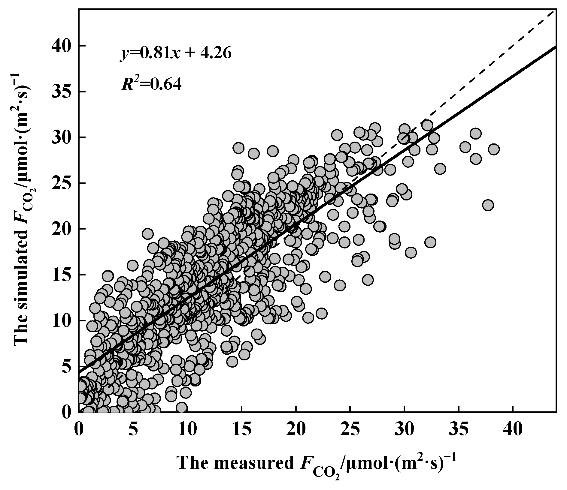
To compare and validate the applicability of the model, linear regression analysis was conducted to compare the relationship between the measured and simulated values of CO2 flux, as shown in Figure 7. t-test analysis showed that there was no significant difference between the simulated and measured values (p < 0.001), with a correlation coefficient R2 of 0.64 for the regression model, indicating that the revised model explains 64% of the variability in rice CO2 flux. Meanwhile, when the flux values were low, the simulated results were consistently higher, suggesting the possible presence of other environmental constraints in such cases. Conversely, when the flux values were high, the simulated results were noticeably lower than the actual levels. In addition, the slope of the regression line was 0.81, with an intercept of 4.26, accounting for 11.1% of the maximum flux value, meeting the accuracy requirements.
4. Conclusions
This study found that the variation range of 30 min CO2 flux in the rice ecosystem was −0.1 to −38.4 μmol·(m2·s)−1, with an average of −12.9 μmol·(m2·s)−1. The highest flux values occurred during the flowering stage of rice, during which the photosynthetic capacity of rice was strong and biological activities were vigorous, resulting in a higher net absorption of CO2. The CO2 flux during the rice growing season displayed a diurnal pattern characterized by an initial increase followed by a decrease. Moreover, there was a sudden abnormal decrease at around 12:00, which could be attributed to the phenomenon of the crop’s midday dormancy. In addition, PAR, T, VPD, Phen, Time, and CO2 concentration were all important factors influencing the rice canopy CO2 flux. When PAR exceeded 800 μmol·(m2·s)−1, T was approximately 31.6 °C, VPD was less than 2.38 KPa, CO2 concentration was below 423.4 μL·L−1, etc., rice CO2 flux was at a relatively high level. The response pattern of rice canopy CO2 flux to various environmental factors was similar to that of stomatal conductance to environmental factors, indicating that canopy and leaf activities under the influence of various environmental factors had similar impact mechanisms. The simulated CO2 flux using the parameterized model was compared with measured values, and it was found that the parameter model established in this study could be used to simulate rice CO2 flux.
Author Contributions
Conceptualization, J.W. (Jinghan Wang) and J.W. (Jiayan Wang); methodology, H.Z., J.W. (Jinghan Wang) and Y.Z.; formal analysis, H.Z. and J.W. (Jiayan Wang); writing—original draft preparation, H.Z., J.W. (Jinghan Wang), J.W. (Jiayan Wang) and Y.Z.; writing—review and editing, H.Z. and J.W. (Jinghan Wang). All authors have read and agreed to the published version of the manuscript.
Funding
This research was funded by the China Postdoctoral Science Foundation (2020M681157).
Institutional Review Board Statement
Not applicable.
Informed Consent Statement
Not applicable.
Data Availability Statement
The data presented in this study are available on request from the corre-sponding author. The data are not publicly available due to privacy.
Conflicts of Interest
The authors declare no conflict of interest.
References
- Fedorov, V.B.; Trucchi, E.; Goropashnaya, A.V.; Waltari, E.; Whidden, S.E.; Stenseth, N.C. Impact of past climate warming on genomic diversity and demographic history of collared lemmings across the Eurasian Arctic. Proc. Natl. Acad. Sci. USA 2020, 117, 3026–3033. [Google Scholar] [CrossRef] [PubMed]
- Zickfeld, K.; Eby, M.; Matthews, H.D.; Weaver, A.J. Setting cumulative emissions targets to reduce the risk of dangerous climate change. Proc. Natl. Acad. Sci. USA 2009, 106, 16129–16134. [Google Scholar] [CrossRef] [PubMed]
- Fan, J.; McConkey, B.G.; Liang, B.C.; Angers, D.A.; Janzen, H.H.; Kröbel, R.; Cerkowniak, D.D.; Smith, W.N. Increasing crop yields and root input make Canadian farmland a large carbon sink. Geoderma 2019, 336, 49–58. [Google Scholar] [CrossRef]
- Lei, H.; Yang, D. Seasonal and interannual variations in carbon dioxide exchange over a cropland in the North China Plain. Glob. Change Biol. 2010, 16, 2944–2957. [Google Scholar] [CrossRef]
- Yue, Y.; Ni, J.; Ciais, P.; Piao, S.; Wang, T.; Huang, M.; Borthwick, A.G.L.; Li, T.; Wang, Y.; Chappell, A.; et al. Lateral transport of soil carbon and land-atmosphere CO2 flux induced by water erosion in China. Proc. Natl. Acad. Sci. USA 2016, 113, 6617–6622. [Google Scholar] [CrossRef]
- Wang, J.; Yu, Q.; Li, J.; Li, L.-H.; Li, X.-G.; Yu, G.-R.; Sun, X.-M. Simulation of diurnal variations of CO2, water and heat fluxes over winter wheat with a model coupled photosynthesis and transpiration. Agric. For. Meteorol. 2006, 137, 194–219. [Google Scholar] [CrossRef]
- Mei, B.; Zheng, X.; Xie, B.; Dong, H.; Zhou, Z.; Wang, R.; Deng, J.; Cui, F.; Tong, H.; Zhu, J. Nitric oxide emissions from conventional vegetable fields in southeastern China. Atmos. Environ. 2009, 43, 2762–2769. [Google Scholar] [CrossRef]
- Chen, H.; Li, H.; Wei, Y.; McBean, E.; Liang, H.; Wang, W.; Huang, J.J. Partitioning eddy covariance CO2 fluxes into ecosystem respiration and gross primary productivity through a new hybrid four sub-deep neural network. Agric. Ecosyst. Environ. 2024, 361, 108810. [Google Scholar] [CrossRef]
- Baldocchi, D.D. Assessing the eddy covariance technique for evaluating carbon dioxide exchange rates of ecosystems: Past, present and future. Glob. Change Biol. 2003, 9, 479–492. [Google Scholar] [CrossRef]
- Huang, Y.; Yu, Y.; Zhang, W.; Sun, W.; Liu, S.; Jiang, J.; Wu, J.; Yu, W.; Wang, Y.; Yang, Z. Agro-C: A biogeophysical model for simulating the carbon budget of agroecosystems. Agric. For. Meteorol. 2009, 149, 106–129. [Google Scholar] [CrossRef]
- Zhao, H.; Huang, J.; Zheng, Y. Observation of ozone deposition flux and its contribution to stomatal uptake over a winter wheat field in eastern China. Atmos. Environ. 2024, 326, 120472. [Google Scholar] [CrossRef]
- Massman, W.J.; Lee, X. Eddy covariance flux corrections and uncertainties in long-term studies of carbon and energy exchanges. Agric. For. Meteorol. 2002, 113, 121–144. [Google Scholar] [CrossRef]
- Falge, E.; Baldocchi, D.; Olson, R.; Anthoni, P.; Aubinet, M.; Bernhofer, C.; Burba, G.; Ceulemans, R.; Clement, R.; Dolman, H.; et al. Gap filling strategies for defensible annual sums of net ecosystem exchange. Agric. For. Meteorol. 2001, 107, 43–69. [Google Scholar] [CrossRef]
- Tong, L.; Wang, X.; Geng, C.; Wang, W.; Lu, F.; Song, W.; Liu, H.; Yin, B.; Sui, L.; Wang, Q. Diurnal and phenological variations of O3 and CO2 fluxes of rice canopy exposed to different O3 concentrations. Atmos. Environ. 2011, 45, 5621–5631. [Google Scholar] [CrossRef]
- Wu, R.J.; Zheng, Y.F.; Hu, C.D. Evaluation of the chronic effects of ozone on biomass loss of winter wheat based on ozone flux-response relationship with dynamical flux thresholds. Atmos. Environ. 2016, 142, 93–103. [Google Scholar] [CrossRef]
- Hu, S.; Li, T.; Wang, Y.; Gao, B.; Jing, L.; Zhu, J.; Wang, Y.; Huang, J.; Yang, L. Effects of free air CO2 enrichment (FACE) on grain yield and quality of hybrid rice. Field Crops Res. 2024, 306, 109237. [Google Scholar] [CrossRef]
- Bonilla-Cordova, M.; Cruz-Villacorta, L.; Echegaray-Cabrera, I.; Ramos-Fernández, L.; Flores del Pino, L. Design of a Portable Analyzer to Determine the Net Exchange of CO2 in Rice Field Ecosystems. Sensors 2024, 24, 402. [Google Scholar] [CrossRef] [PubMed]
- Demyan, M.S.; Ingwersen, J.; Funkuin, Y.N.; Ali, R.S.; Mirzaeitalarposhti, R.; Rasche, F.; Poll, C.; Müller, T.; Streck, T.; Kandeler, E.; et al. Partitioning of ecosystem respiration in winter wheat and silage maize—Modeling seasonal temperature effects. Agric. Ecosyst. Environ. 2016, 224, 131–144. [Google Scholar] [CrossRef]
- Xu, J.; Zheng, Y.; Mai, B.; Zhao, H.; Chu, Z.; Huang, J.; Yuan, Y. Simulating and partitioning ozone flux in winter wheat field: The Surfatm-O3 model. China Environ. Sci. 2018, 38, 455–470. (In Chinese) [Google Scholar]
- Murata, N.; Takahashi, S.; Nishiyama, Y.; Allakhverdiev, S.I. Photoinhibition of photosystem II under environmental stress. Biochim. Biophys. Acta BBA Bioenerg. 2007, 1767, 414–421. [Google Scholar] [CrossRef]
- Pérez, I.A.; Sánchez, M.L.; García M, Á.; Pardo, N.; Fernández-Duque, B. The influence of meteorological variables on CO2 and CH4 trends recorded at a semi-natural station. J. Environ. Manag. 2018, 209, 37–45. [Google Scholar] [CrossRef] [PubMed]
- Tong, L.; Xiao, H.; Qian, F.; Huang, Z.; Feng, J.; Wang, X. Daytime and phenological characteristics of O3 and CO2 fluxes of winter wheat canopy under short-term O3 exposure. Water Air Soil Pollut. 2016, 227, 1–14. [Google Scholar] [CrossRef]
- Fares, S.; McKay, M.; Holzinger, R.; Goldstein, A.H. Ozone fluxes in a Pinus ponderosa ecosystem are dominated by non-stomatalprocesses: Evidence from long-term continuous measurements. Agric. For. Meteorol. 2010, 150, 420–430. [Google Scholar] [CrossRef]
- Stella, P.; Personne, E.; Loubet, B.; Lamaud, E.; Ceschia, E.; Béziat, P.; Bonnefond, J.M.; Irvine, M.; Keravec, P.; Mascher, N.; et al. Predicting and partitioning ozone fluxes to maize crops from sowing to harvest: The Surfatm-O3 model. Biogeosciences 2011, 8, 2869–2886. [Google Scholar] [CrossRef]
- Zhang, W.; Feng, Z.; Wang, X.; Liu, X.; Hu, E. Quantification of ozone exposure- and stomatal uptake-yield response relationships for soybean in Northeast China. Sci. Total Environ. 2017, 599–600, 710–720. [Google Scholar] [CrossRef]
Figure 1.
The daily variations in meteorological factors during the rice growing season.

Figure 2.
Diurnal variation in CO2 concentration (mean ± standard error) during the rice growing season.
Figure 2.
Diurnal variation in CO2 concentration (mean ± standard error) during the rice growing season.

Figure 3.
Time series variation in daytime CO2 flux during the rice growing season.

Figure 4.
Seasonal variation in daytime CO2 flux during the rice growing season.

Figure 5.
Diurnal variation in CO2 flux (mean ± standard error) during the rice growing season.

Figure 6.
The limiting effects of different climatic factors on rice CO2 flux.

Figure 7.
Validation of rice CO2 flux model.


Table 1.
Parameter values of stress coefficient in rice CO2 flux model.
| Stress Coefficient | Parameter | Unit | Parameter Value | |
|---|---|---|---|---|
| Before Revision | After Revision | |||
| — | μmol·(m2·s)−1 | 41.4 | 38.4 | |
| fmin | — | — | 0.01 | 0.01 |
| fPAR | L | — | 0.0026 | 0.0027 |
| ftemp | tmin | °C | 20.2 | 16.2 |
| topt | °C | 31.6 | 31.7 | |
| tmax | °C | 40.5 | 40.9 | |
| fVPD | VPDmax | KPa | 1.8 | 2.38 |
| VPDmin | KPa | 3.0 | 4.22 | |
| fphen | Dayc | D | 93 | 99 |
| Dayd | D | 102 | 109 | |
| c1 | — | 0.0043 | 0.0084 | |
| d1 | — | 0.60 | 0.20 | |
| c2 | — | −0.022 | −0.0143 | |
| d2 | — | 3.28 | 2.54 | |
| fTime | e | — | 16.6 | 16.7 |
| f | — | 13.8 | 14.4 | |
| μL·L−1 | — | 486.2 | ||
| μL·L−1 | — | 423.4 | ||
Disclaimer/Publisher’s Note: The statements, opinions and data contained in all publications are solely those of the individual author(s) and contributor(s) and not of MDPI and/or the editor(s). MDPI and/or the editor(s) disclaim responsibility for any injury to people or property resulting from any ideas, methods, instructions or products referred to in the content. |
© 2024 by the authors. Licensee MDPI, Basel, Switzerland. This article is an open access article distributed under the terms and conditions of the Creative Commons Attribution (CC BY) license (https://creativecommons.org/licenses/by/4.0/).
Share and Cite
MDPI and ACS Style
Wang, J.; Wang, J.; Zhao, H.; Zheng, Y. Observation and Simulation of CO2 Fluxes in Rice Paddy Ecosystems Based on the Eddy Covariance Technique. Atmosphere 2024, 15, 517. https://0-doi-org.brum.beds.ac.uk/10.3390/atmos15050517
AMA Style
Wang J, Wang J, Zhao H, Zheng Y. Observation and Simulation of CO2 Fluxes in Rice Paddy Ecosystems Based on the Eddy Covariance Technique. Atmosphere. 2024; 15(5):517. https://0-doi-org.brum.beds.ac.uk/10.3390/atmos15050517
Chicago/Turabian StyleWang, Jinghan, Jiayan Wang, Hui Zhao, and Youfei Zheng. 2024. "Observation and Simulation of CO2 Fluxes in Rice Paddy Ecosystems Based on the Eddy Covariance Technique" Atmosphere 15, no. 5: 517. https://0-doi-org.brum.beds.ac.uk/10.3390/atmos15050517
Note that from the first issue of 2016, this journal uses article numbers instead of page numbers. See further details here.